Iron-Binding Ligands in the Southern California Current System: Mechanistic Studies

Bundy, Randelle M.; Jiang, Mingshun; Carter, Melissa; Barbeau, Katherine A.

doi:10.3389/fmars.2016.00027

ORIGINAL RESEARCH article

Front. Mar. Sci., 15 March 2016
Sec. Marine Biogeochemistry
Volume 3 - 2016 | https://doi.org/10.3389/fmars.2016.00027

Iron-Binding Ligands in the Southern California Current System: Mechanistic Studies

Randelle M. Bundy¹^*

Mingshun Jiang²

Melissa Carter¹

Katherine A. Barbeau¹

¹Geosciences Research Division, Scripps Institution of Oceanography, University of California, San Diego, San Diego, CA, USA
²Harbor Branch Oceanographic Institute, Florida Atlantic University, Fort Pierce, FL, USA

The distributions of dissolved iron and organic iron-binding ligands were examined in water column profiles and deckboard incubation experiments in the southern California Current System (sCCS) along a transition from coastal to semi-oligotrophic waters. Analysis of the iron-binding ligand pool by competitive ligand exchange-adsorptive cathodic stripping voltammetry (CLE-ACSV) using multiple analytical windows (MAWs) revealed three classes of iron-binding ligands present throughout the water column (L₁−L₃), whose distributions closely matched those of dissolved iron and nitrate. Despite significant biogeochemical gradients, ligand profiles were similar between stations, with surface minima in strong ligands (L₁ and L₂), and relatively constant concentrations of weaker ligands (L₃) down to 500 m. A phytoplankton grow-out incubation, initiated from an iron-limited water mass, showed dynamic temporal cycling of iron-binding ligands. A biological iron model was able to capture the patterns of the strong ligands in the grow-out incubation relatively well with only the microbial community as a biological source. An experiment focused on remineralization of particulate organic matter showed production of both strong and weak iron-binding ligands by the heterotrophic community, supporting a mechanism for in-situ production of both strong and weak iron-binding ligands in the subsurface water column. Photochemical experiments showed a variable influence of sunlight on the degradation of natural iron-binding ligands, providing some evidence to explain differences in surface ligand concentrations between stations. Patterns in ligand distributions between profiles and in the incubation experiments were primarily related to macronutrient concentrations, suggesting microbial remineralization processes might dominate on longer time-scales over short-term changes associated with photochemistry or phytoplankton growth.

Introduction

Dissolved iron (dFe) is an essential trace element for microbial growth in large areas of the ocean (Morel and Price, 2003). Phytoplankton growth in high nutrient low chlorophyll (HNLC) regions is especially susceptible to iron (Fe) limitation in surface waters (Martin et al., 1991). Some coastal eastern boundary upwelling regions such as the California Current System (CCS) can also have a range of Fe-limiting conditions, from the nearshore continental shelf to the transition zone extending 10–250 km offshore (Hutchins et al., 1998; King and Barbeau, 2007, 2011; Biller and Bruland, 2014). Iron (Fe) is necessary for primary production, but it is often scarce and almost always associated with a heterogeneous pool of organic ligands with varying reactivities (Rue and Bruland, 1995; van den Berg, 1995; Wu and Luther, 1995). Bacteria and phytoplankton must therefore use an assortment of cellular tools in order to access dFe from this diverse organic matter matrix (Granger and Price, 1999; Hutchins et al., 1999; Maldonado and Price, 1999), and determining the chemical nature of these unknown organic ligands is important for understanding the mechanisms of Fe-acquisition in the ocean.

Although dFe-binding ligands can be directly isolated from seawater (e.g., Mawji et al., 2008), dFe-binding organic ligands are most commonly detected using indirect electrochemical methods such as competitive ligand exchange-adsorptive cathodic stripping voltammetry (CLE-ACSV), which classifies ligands based on their concentrations and binding strengths (see review by Gledhill and Buck, 2012). The strengths of some of the strongest ligands identified in the ocean by electrochemical methods are nearly identical to model siderophores found in culture media. Likely, the dFe-binding ligands measured by electrochemistry could range from highly specific low molecular weight siderophore-type ligands to large macromolecules with only weak dFe-binding (Gledhill and Buck, 2012). The strongest dFe-binding ligands appear to be largely biologically produced, both as a strategy for combating Fe-limitation (Maldonado et al., 2002; Buck et al., 2010; Mawji et al., 2011) and for preventing Fe precipitation (Reid et al., 1993; Kondo et al., 2008). Cultured bacteria have been shown to produce siderophores (Amin et al., 2009; Vraspir and Butler, 2009), and CLE-ACSV measurements made in conjunction with high performance liquid chromatography (HPLC) methods have identified siderophores associated with natural bacteria assemblages (Gledhill et al., 2004; Mawji et al., 2011). Microbial communities may also be an in-situ source of weaker ligands to the subsurface water column during the remineralization of particulate organic matter (Boyd et al., 2010). It appears that bacteria may be a source of both strong and weak dFe-binding ligands in certain conditions, but it is less certain whether there are other biological processes affecting the distribution of dFe-binding ligands. Ligand maxima in the water column, for example, are often associated with the chlorophyll a maxima (Boye et al., 2001, 2005, 2006; Croot et al., 2004; Wagener et al., 2008; Ibisanmi et al., 2011). However, it is still not clear from field studies what mechanisms may cause the elevated ligand concentrations at this depth in the water column.

In addition to biological changes to the ligand pool, photochemistry can also affect the concentration and strength of dFe-binding ligands. Laboratory studies have shown that some siderophores can be degraded by natural sunlight when bound to dFe, and their binding strength is subsequently decreased (Barbeau et al., 2001, 2003; Barbeau, 2006). This mechanism has been invoked to describe the minima in strong ligands often seen in surface waters (Gledhill and Buck, 2012). However, field studies to date have demonstrated mixed results with respect to photochemical degradation of natural dFe-binding ligands (Powell and Wilson-Finelli, 2003; Rijkenberg et al., 2006). Despite varied results in the field, modeling studies routinely invoke a photochemical sink of dFe-binding ligands in surface waters (Parekh et al., 2005; Fan, 2008; Tagliabue et al., 2009; Tagliabue and Volker, 2011; Jiang et al., 2013).

Although data suggests the presence of strong and weak dFe-binding ligands throughout the water column, the mechanisms linking ligand distributions to sources and sinks have not been well studied. This is despite the advent of large-scale projects such as GEOTRACES, which have vastly increased the number and spatial coverage of ligand measurements (Thuróczy et al., 2010, 2011a,b; Sander et al., 2014; Buck et al., 2015; Gerringa et al., 2015). Data in the Pacific is still forthcoming, but measurements from both Buck et al. (2015) and Gerringa et al. (2015) in the Atlantic, show the presence of strong dFe-binding ligands (log $K_{F e L, F e^{'}}^{c o n d}$ > 12) in the entire water column. Estimates from a meridional transect by Gerringa et al. (2015) suggest that these ligands are potentially long-lived relative to dFe (residence time of 779–1039 years), perhaps partly explaining their ubiquitous presence. These large datasets are critical not only for understanding ligand sources and sinks, but also for informing current biogeochemical modeling efforts, which are increasingly incorporating dFe-binding ligands (Archer and Johnson, 2000; Moore et al., 2004; Parekh et al., 2005; Fan, 2008; Moore and Braucher, 2008; Tagliabue et al., 2009; Tagliabue and Volker, 2011; Jiang et al., 2013; Boyd and Tagliabue, 2015).

Modeling studies have shown that incorporating dFe-binding ligand dynamics can have a large effect on the observed dFe concentrations (Tagliabue et al., 2014). Implementing ligand dynamics in biogeochemical models has so far been challenging however, because a spectrum of dFe-binding ligand strengths has been found to exist in seawater with a range of conditional stability constants (log $K_{F e L, F e^{'}}^{c o n d}$ ) from 9.0 to 14.0 (Hunter and Boyd, 2007; Gledhill and Buck, 2012). Most studies to date have concentrated on measuring one particular ligand class in this spectrum, often denoted as strong “L₁” ligands or weaker “L₂” ligands. Based on recommendations from Gledhill and Buck (2012) some recent studies however, have focused on measuring several dFe-binding ligand classes in the same sample using CLE-ACSV with multiple analytical windows (MAWs; Bundy et al., 2014a,b; Sander et al., 2014; Mahmood et al., 2015) or displaying their data in terms of absolute rather than relative log $K_{F e L, F e^{'}}^{c o n d}$ (Buck et al., 2015). These approaches have shed some light on the potential sources and sinks of both stronger and weaker ligands in the water column, but thus far MAW analysis has been restricted to the benthic boundary layer (Bundy et al., 2014a,b) and surface waters (Bundy et al., 2014a,b; Sander et al., 2014; Mahmood et al., 2015). In Bundy et al. (2014a,b), a range of dFe-binding ligand strengths were detected and denoted as L₁–L₄. These ligand classes span the range of ligand strengths that have been observed in many other studies (Gledhill and Buck, 2012), but the processes associated with L₁–L₄ distributions in the subsurface water column are still uncertain. This study makes the first upper ocean profile measurements of dFe-binding organic ligands utilizing MAW CLE-ACSV, and seeks to link profile data with mechanistic deckboard dFe speciation studies carried out on the same cruise in the southern California Current region, also employing MAW CLE-ACSV.

Methods

Sampling Region and Environmental Context

Samples for this study were collected as part of the California Current Ecosystem (CCE) Long-Term Ecological Research (LTER) program (http://cce.lternet.edu/) in the southern California Bight (Figure 1) on-board the R/V Melville in June–July 2011. This cruise was a CCE-LTER process cruise, which uses drifters in a Langrangian platform to follow distinct water masses (Landry et al., 2009; Krause et al., 2015). Each series of stations sampled within the same water mass were denoted as a “cycle” (Brzezinski et al., 2015; Krause et al., 2015). However, only one station from each cycle was sampled in this particular study, so sampling locations will simply be referred to as stations. Each station has been given the same number as the cycle to which it belongs (for example, station 1 was part of cycle 1) in order to compare to other studies from the same cruise (e.g., Brzezinski et al., 2015; Krause et al., 2015).

FIGURE 1

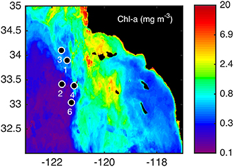
Figure 1. Sampling locations for water column profiles and incubation experiments during the June/July 2011 cruise. Stations were sampled in the coastal (3, 4), frontal (1, 6), and oceanic (2) side of a distinct frontal feature (Brzezinski et al., 2015; Krause et al., 2015) shown over the averaged chlorophyll a (chl-a; mg m⁻³) for the month of July in 2011.

Sampling and Storage

All trace-metal clean samples were collected either using single Teflon-coated 12 L GO-Flo bottles (General Oceanics) mounted directly on non-metallic hydroline or 5 L X-Niskin bottles (Ocean Test Equipment) mounted on a powder-coated rosette deployed on non-metallic hydroline (Cutter and Bruland, 2012) according to the methods described in Brzezinski et al. (2015). Filtered samples for dFe analysis were placed in 250 mL low-density polyethylene (LDPE) bottles, acidified to pH 1.8 (Optima HCl) and stored for at least 3 months until analysis in the lab. Samples collected for dFe-binding ligands were either run immediately (within 3 days) or stored frozen at −20° C until analysis. Results for fresh vs. frozen analyses of dFe-binding ligands have been shown to be indistinguishable in previous studies (Buck et al., 2012).

Filtered samples for silicate (Si(OH)₄), phosphate (PO $_{4}^{3 -}$ ), nitrate (nitrate+nitrite; denoted as NO $_{3}^{-}$ ), and chlorophyll a (chl a) were taken from the standard CTD rosette cast and on-board incubation experiments. Nutrient samples were collected in 40 ml polypropylene centrifuge tubes (Fisher Scientific) and frozen at −20°C before analysis. Chl a and phytoplankton pigment samples were placed in dark bottles and filtered onto glass fiber filters (GF/F filters, Fisher Scientific). Chl a samples were subsequently placed in acetone and analyzed on-board. Pigment samples were put in cryovials (Nalgene) and stored in liquid nitrogen until analysis in the lab. Microscopy samples for phytoplankton cell counts were collected in 50 mL glass vials and stored in 1% tetraborate buffered formalin until analysis.

Nutrients and Phytoplankton

Chl a samples from the depth-profiles and incubation experiments were run immediately on-board the ship, after being extracted for 24 h in acetone at −20°C. Chl a samples were analyzed using a Turner Designs 10-AU Fluorometer, fitted with a red-sensitive photomultiplier tube. Phytoplankton pigment samples were analyzed by HPLC according to Zapata et al. (2000). Macronutrients from the water column profiles and incubation experiments were analyzed by the Marine Science Institute Analytical Lab at the University of California Santa Barbara (http://msi.ucsb.edu/services/analytical-lab) using a Lachat QuickChem 8000. Samples for phytoplankton cell counts were first adjusted by volume to 60 mL before settling in a 50 mL Utermöhl settling chamber. They were then counted using a Zeiss phase-contrast inverted light microscope at 200x magnification (Utermöhl, 1958; UNESCO, 1981). Phytoplankton were classified by genera or the following broad categories: Chaetoceros spp., Pseudo-nitzschia spp., other diatoms (>10 μm), dinoflagellates, flagellates (< 10 μm), and ciliates. The sample volume enumerated ranged from 5.6 to 1.1 mL (1/9 of slide) and detectable cell abundances were between 245 and 1227 cells L⁻¹, depending on the volume settled.

Dissolved Iron

The dFe was analyzed by flow injection analysis (FIA) after complete reduction of the dFe with sulfite according to King and Barbeau (2007, 2011). This method has been shown to yield accurate results with respect to SAFe (S1 and D2) and GEOTRACES (GS) consensus samples, and has a detection limit of 0.07 nmol L⁻¹ (three time the standard deviation of the blank, n = 72). Values obtained for S1 (0.11 ± 0.02 nmol L⁻¹, n = 39), D2 (0.93 ± 0.07 nmol L⁻¹, n = 36), and GS (0.51 ± 0.02 nmol L⁻¹, n = 12) compare well to the most recent consensus values (http://es.ucsc.edu/~kbruland/GeotracesSaFe/kwbGeotracesSaFe.html).

Dissolved Iron-Binding Ligands

The analysis of dFe-binding ligands was completed using (CLE-ACSV). This method has been used extensively for determining the concentration and binding strengths of dFe-binding ligands in seawater (see a recent review by Gledhill and Buck, 2012). Briefly, a natural sample is titrated with dFe in order to saturate the natural ligands. Then, a well-characterized electroactive ligand is added, in this case salicylaldoxime (SA). SA competes with the natural ligands for dFe, and the Fe(SA)_x complex is deposited on the mercury drop, and analyzed using adsorptive cathodic stripping voltammetry (ACSV) on a hanging mercury drop electrode (BioAnalytical Systems, Incorporated).

Titrations were performed by first adding 50 μl of a 1.5 mol L⁻¹ boric acid-ammonium buffer (sample pH = 8.2, NBS scale) to 10 mL aliquots of the sample. Next, 0–25 nmol L⁻¹ dFe (range varied depending on the detection window) was added to 11 separate conditioned Teflon vials (Savillex) containing the sample and buffer. The buffer and dFe were left to equilibrate with the natural ligands in the sample for 2 h, before adding the appropriate concentration of SA depending on the detection window (17.7, 25.0, or 32.3 μmol L⁻¹ SA). The SA was equilibrated for 15 min before each aliquot was run separately using ACSV with a 150 s deposition time. All electrochemical parameters were the same as have been reported previously (Rue and Bruland, 1995; Buck et al., 2007), and all constants for SA were updated to the most recent calibration reported by Abualhaija and van den Berg (2014). Peak heights were determined using ECDSOFT and the sensitivity was optimized in ProMCC (Omanović et al., 2014). Results from selected samples at a single analytical window were also confirmed using BackCalc. Ligand concentrations and strengths were calculated both by traditional linearization techniques and using a unified multi-window approach (Hudson et al., 2003). The results between these two methods compared well when initial guesses from linearization techniques were used (Bundy et al., 2014a). However, a common sensitivity ratio (R_AL) has not yet been empirically determined for Fe MAW CLE-ACSV, because of a paucity of MAW data for Fe from a variety of lab groups and is an essential parameter in the unified multi-window approach (Mahmood et al., 2015). Since a rigorous intercomparison has yet to be completed for dFe-binding ligand titration data using new numerical methods, and an empirical R_AL has not yet been published, traditional linearization approaches were used in this study and are reported as the average between the concentration and strengths determined by a Ružić/van den Berg linearization (Mantoura and Riley, 1975) and Scatchard linearization (Scatchard, 1949). Although linearization approaches generally have higher error functions than numerical models of metal speciation when tested with artificial data (Pižeta et al., 2015), linear models still compare well with numerical speciation models when the sensitivity is optimized.

The concentration of the added ligand determines the detection window of the method, or the strength of the ligands that can be detected. A higher detection window targets stronger ligands, while a lower window targets weaker ligands. For this study, three different concentrations of SA were used, or three detection windows, in order to examine several distinct ligand classes ([SA] = 17.7, 25.0, and 32.3 μmol L⁻¹, α_{Fe(SA)_x} = 75, 115, and 162). One ligand class was detected at each analytical window, except the lowest detection window ([SA] = 17.7 μmol L⁻¹) where two ligand classes were detected. Each subsequent titration was performed with at least three points of overlap from the previous titration (in terms of the dFe additions), with the lowest analytical window having the highest dFe additions at the end of the titration. The strongest ligand class (L₁) was determined at the highest detection window (32.3 μmol L⁻¹ SA), the next ligand class (L₂) was detected at the middle detection window (25.0 μmol L⁻¹ SA) and the weakest ligand classes (L₃ and L₄) were detected at the lowest detection window (17.7 μmol L⁻1 SA). The conditional stability constants defined for each ligand class was defined as log $K_{F e L_{1}, F e^{'}}^{c o n d} \geq$ 12.0 for L₁, log $K_{F e L_{2}, F e^{'}}^{c o n d} =$ 11.0–12.0 for L₂, log $K_{F e L_{3}, F e^{'}}^{c o n d} =$ 10.0–11.0 for L₃, and log $K_{F e L_{4}, F e^{'}}^{c o n d} \leq$ 10.0 for L₄ (Bundy et al., 2014a,b).

Experimental Set-Up

Biological Incubation Experiments

Two experiments were conducted in this study to address biological sources of dFe-binding ligands in the CCS: one Fe addition phytoplankton grow-out experiment (experiment 1) and one remineralization experiment (experiment 2), which immediately followed the termination of the grow-out experiment. Both experiments were conducted at station 3 from water collected at 30 m in the subsurface chl a maximum (Figure 1). Whole seawater was collected and homogenized in a clean 50 L carboy before being aliquoted into acid-cleaned 4 L polycarbonate (PC) bottles. Experiments 1 and 2 contained a set of three unamended controls (Control A, B, and C) and three +Fe bottles (5 nmol L-1 FeCl3; +Fe A, B, and C). All six bottles for experiments 1 and 2 were placed in on-deck flow-through incubators screened to 30% light levels, which were similar to in-situ light and temperature conditions. Bottles for experiment 2 were placed in 2 heavy-duty black garbage bags and also placed in the on-deck flow-through incubator. Experiment 1 was terminated after 6 days, and experiment 2 was terminated after 3 days. Experiment 2 was initiated using the phytoplankton biomass that had accumulated in the controls and +Fe treatments at the end of experiment 1, and were simply placed in the dark following the termination of the light portion of experiment 1 on day 6.

Samples for chl a, macronutrients [NO₃₋, PO $_{4}^{3 -}$ , and Si(OH)₄], phytoplankton pigments, phytoplankton cell counts, dFe, and dFe-binding ligands were taken from experiment 1. Experiment 2 was only sampled for dFe and dFe-binding ligands. Samples for chl a were taken every day from all six bottles in experiments 1, and macronutrients were sampled every 2 days from all six bottles. Pigment concentrations and phytoplankton cell counts were sampled on day 0 from the 50 L carboy (initial conditions) and day 6 (final conditions) in all controls and +Fe bottles. The dFe and dFe-binding ligands were sampled every day in experiment 1, but only from one bottle of each treatment until day 6, when all bottles were sampled. For example, Control A and +Fe A bottles were sampled on days 1, 4, and 6, Control B and +Fe B were sampled on days 2, 5, and 6, and Control C and +Fe C were sampled on days 3 and 6. The dFe and ligands for experiment 2 were sampled on day 0, and then on day 3 (final conditions) from all treatments. A subset of the data from experiment 1 is also shown in Brzezinski et al. (2015).

Photochemical Experiments

Photochemical experiments were performed at stations 1, 2, and 6 at the depth of the chl a maximum (30, 70, and 20 m, respectively). Trace metal clean seawater was collected before sunrise and filtered in-line with a 0.2 μm Acropak-200 filter. Filtered seawater was homogenized in a clean carboy and dispensed into four conditioned quartz flasks with Teflon stoppers (Quartz Scientific). Two of the flasks were wrapped tightly in aluminum foil for the dark controls. All four flasks were placed in a shallow plastic tray coupled to the on-deck flow-through incubators and left in the natural sunlight for 12 h. Samples for dFe and dFe-binding ligands were taken randomly from one of the dark flasks for the initial time-point, and from each bottle (Dark A, B and Light A, B) at the end of the 12 h.

Modeling

A biological Fe model developed for the Southern Ocean (Jiang et al., 2013) was modified to test the experimental results of incubation experiment 1. The model resolves the classical food web and microbial loop, including three types of nutrients [NO $_{3}^{-}$ , Si(OH)₄, Fe] and two types of dFe-binding ligands (L₁, L₂). The Fe cycle is simulated with five Fe species including dissolved inorganic Fe (Fe'), dissolved Fe bound to the two stronger ligand classes (FeL₁ and FeL₂), and colloidal Fe and particulate Fe. The ligand dynamics include most of the key processes including bio-complexation, photo-degradation, thermal dissociation, L₁ ligand production by bacteria during Fe-stress conditions, and L₂ ligand production by the remineralization of particulate organic matter and via photochemical degradation of L₁. No ligand production due to phytoplankton growth or zooplankton grazing is included (e.g., Barbeau et al., 1996; Sato et al., 2007), and there was no attempt to model the weakest ligand classes (L₃ and L₄). The model has been tested with data from shipboard grow-out incubation experiments and in-situ data during two cruises in the Antarctic Peninsula area, through zero-dimensional and one-dimensional experiments, respectively (Jiang et al., 2013). In this project, some of the model parameters were adjusted to the lower macronutrient conditions in the southern CCE (Table 1).

TABLE 1

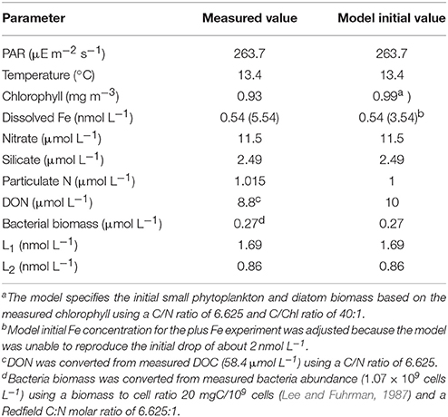
Table 1. Ancillary measurements made in the water column as part of the CCE-LTER program for biological experiment 1 and used as initial parameters in the model.

Statistical Analyses

A Pearson's correlation analysis was performed using the Statistics Toolbox in Matlab with all data from CTD profiles and the incubation experiment, including the dFe and ligand data. Missing values were replaced using a regression with depth for the profile data, or a regression with time for the incubation data and all correlation coefficients are reported at the 95% confidence interval.

Results

Water Column Profiles

Each station was loosely grouped as coastal, frontal or oceanic based on physical characteristics. CTD data was obtained for all stations (1–4 and 6, data not shown), and dFe and dFe-binding ligand depth profiles were collected for stations 1, 2, 4, and 6. Stations 3 and 4 were classified as coastal stations, stations 1 and 6 were frontal stations, and station 2 was considered oceanic, based on defined water mass characteristics in relation to a persistent frontal feature between cyclonic and anticyclonic eddies that was sampled in this region as part of the CCE-LTER program (Brzezinski et al., 2015; Krause et al., 2015). The depth and magnitude of the chl a maximum and nitracline corresponded well with these groupings, for the stations shown in Figure 2 where dFe and ligands were also sampled. Coastal station 4 (Figure 2A) was characterized by a relatively shallow biomass maximum (< 50 m) and nitracline (< 20 m). Very high chl a concentrations were observed at station 4 (up to 9 μg L⁻¹), corresponding with almost complete drawdown of NO $_{3}^{-}$ in surface waters. The frontal stations (Figures 2C,E) were hydrographically similar to the coastal stations but had a slightly deeper nitracline (40–50 m) and lower [chl a]. The oceanic station (station 2, Figure 2G) had a much deeper nitracline (> 50 m) and a deep chl a maximum relative to the coastal stations.

FIGURE 2

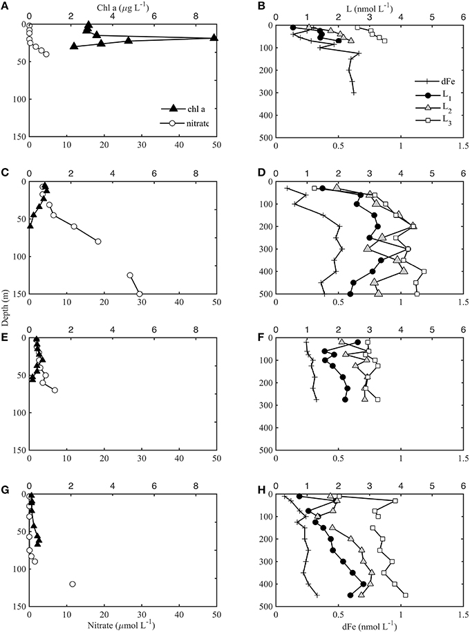
Figure 2. Chl a and nitrate (nitrate+nitrite) bottle samples shown in left panels for coastal station 4 (A), frontal stations 1 (C), and 6 (E), and oceanic station 2 (G) according to characteristics defined in Krause et al. (2015). The dFe (+) and ligand concentrations (L₁ black circles, L₂ gray triangles, L₃ white squares) for the corresponding station are shown in right panels (B,D,F,H). Note the different depth scales of left and right panels.

The [dFe] ranged from < 0.3 nmol L⁻¹ in surface waters to ~0.8 nmol L⁻¹ at 500 m in the coastal station (Figure 2B). DFe in the southern CCS is characterized by low concentrations offshore and a deep ferricline, often deeper than 100 m (King and Barbeau, 2011). The dFe-binding ligands show a similar pattern to dFe (Figure 2). The strongest ligands (L₁, log $K_{F e L_{1}, F e^{'}}^{c o n d} \geq$ 12.0) were present throughout the water column down to 500 m (the deepest depth sampled). Most of the profiles showed a subsurface maxima in L₁ associated with the biomass maxima and then minima, before increasing slightly again at depths below 100 m. Although there were elevated L₁ concentrations at the chl a maxima, there were not higher ligand concentrations associated with the large bloom at station 4 (Figures 2A,B). Three of the four stations showed a minimum in L₁ in surface waters (Figures 2B,D,H), but frontal station 6 had elevated L₁ concentrations at the shallowest depth sampled (20 m, Figure 2F). There is also some evidence at the base of the profiles that L₁ might begin to decline below 500 m, but it is difficult to determine without more sampling depths. For a detailed tabulation of all dFe and ligand profile data see the Supplementary Information (SI-1).

L₂ ligands (log $K_{F e L_{2}, F e^{'}}^{c o n d} =$ 11.0–12.0) were present in slightly higher concentrations than L₁ throughout most of the water column, but had a similar distribution with depth. There is also some evidence that L₂ began to decrease below 400 m at stations 1 and 2, but more sampling depths would be needed to confirm this pattern in deep waters. The L₂ concentration was greatest at frontal station 1 (ranging from 1.5 to 4.2 nmol L⁻¹) compared to the other three stations where L₂ did not exceed 3 nmol L⁻¹. This matched the pattern in dFe and other ligand concentrations, perhaps due to enhanced mixing associated with the frontal zone at this station (Krause et al., 2015). L₃ was relatively distinct from the stronger ligands. [L₃] remained mostly constant throughout the water column, with a few exceptions in surface waters (Figures 2B,D,F,H). [L₃] was higher at the coastal station (station 4) and oceanic station (station 2) than in the frontal region. The highest concentrations of weaker ligands (L₃) in the upper 100 m were found in the oceanic station (stations 2), and the lowest concentrations of weaker ligands were in the frontal waters at stations 1 and 6. On average, this pattern was opposite for the stronger ligands. No L₄ ligands were detected in any of the profiles at any of the depths sampled. Pearson's correlation analysis for the profile data showed the strongest correlations between each of the ligand classes and nitrate (Supplementary Information SI-2), while relatively strong negative correlations were also observed with some of the variables that decrease with depth such as oxygen.

Biological Ligand Production Experiments

Incubation Experiment 1

Experiment 1 was sampled at 30 m from an aged, upwelled water mass that had likely originated nearshore near Point Conception (Brzezinski et al., 2015; Krause et al., 2015). The initial conditions for the experiment had relatively elevated macronutrient concentrations (11.5 μmol L-1 NO $_{3}^{-}$ ; Figure 3A) and dFe (0.54 nmol L-1). Thus, the phytoplankton community was likely not macronutrient limited. Little NO $_{3}^{-}$ was drawn-down in controls, but significant macronutrient drawdown was observed by day 4 of the experiment in +Fe treatments (Figure 3B). The macronutrient drawdown was accompanied by a significant increase in chl a biomass in +Fe treatments compared to controls by day 6 (t-test, p < 0.05). Although the initial phytoplankton community was relatively diverse (Figure 3D), the increase in biomass by day 6 was almost entirely due to an increase in the abundance of diatoms, mostly Pseudo-nitzschia spp. (Figure 3D). The increase in diatoms was apparent both from cell counts (Figure 3D) and from elevated fucoxanthin pigment concentrations compared to initial conditions (Brzezinski et al., 2015). Although the total biomass was much higher in +Fe treatments, the phytoplankton community structure was very similar between the controls and +Fe treatments (Figure 3D). Even though the composition of the phytoplankton community was not significantly different between controls and +Fe treatments, the evolution of NO $_{3}^{-}$ compared to dFe (NO $_{3}^{-}$ : dFe; μmol L-1: nmol L-1) over the course of the experiment was drastically different in controls and +Fe bottles (Figure 3C). Previous work in this region has shown that NO $_{3}^{-}$ (μmol L⁻¹): dFe (nmol L⁻¹) ratios greater than 12 are indicative of Fe-limitation of the diatom community (King and Barbeau, 2007). The initial water mass contained a NO $_{3}^{-}$ : dFe ratio of 21.5, likely indicating that the diatom community was initially Fe-limited. However, the 5 nmol L⁻¹ dFe addition in +Fe bottles appeared to alleviate this Fe-limitation based on the NO $_{3}^{-}$ : dFe ratios observed over the course of the experiment (Figure 3C), and the increase in biomass by day 6 (Figure 3B).

FIGURE 3

Figure 3. Incubation data from incubation experiment 1 at station 3. Chlorophyll a (chl a) and nitrate (nitrate+nitrite) distributions in the water column at station 3 (A). Chl a and nitrate concentrations during the incubation experiment, where * indicates a significance difference in chl a biomass on day 6 (B; t-test, p < 0.05). Nitrate:dFe ratios throughout the incubation experiment (C), and phytoplankton cell counts for controls and +Fe treatments (D). Error bars in panels (A, B, D) represent the standard deviation from the averages of controls (A, B, C) and +Fe treatments (FeA, FeB, FeC) at each time-point.

Although the phytoplankton biomass response differed between controls and +Fe treatments, the temporal pattern of dFe-binding ligands was very similar (Figure 4), especially when considering the variability between bottle replicates on day 6. Most of the dFe was drawn-down in +Fe treatments after day 4 (Figure 4A), concomitant with the increase in phytoplankton biomass and decrease in NO $_{3}^{-}$ . The dFe decreased slightly in controls, likely due to a combination of uptake and scavenging to the walls of the bottles. The strongest ligands (L₁) increased in both controls and +Fe treatments from days 0 to 1, and then remained relatively constant for the remainder of the experiment, with slightly higher ligand concentrations on day 6 in two of the +Fe bottles (Figure 4B). L₂ ligands increased relatively consistently over the 6 days of the experiment (Figure 4C). The weaker ligands showed distinct temporal patterns compared to the stronger ligands, with L₃ slowly decreasing during the sampling period and L₄ ligands only appearing on days 4–6 (Figures 4D,E). Significant differences in ligand classes on each day of incubation experiment 1 were determined by accounting for the average percent standard deviation between replicate bottles that was observed on day 6 rather than from replicate titrations since only one bottle from each treatment was measured each day. The average percent standard deviation from replicate bottles (21% for L₁, 27% for L₂, 37% for L₃, and 21% for L₄) was higher than the standard deviations observed between titrations (9% for L₁, 12% for L₂, 13% for L₃, and 14% for L₄). The average ligand concentrations for each ligand class on day 6 were not statistically distinct in controls and +Fe treatments (t-test, p > 0.05), but certain days throughout the grow-out showed statistically significant differences in ligand concentrations (Figure 4). In general however, the overall temporal ligand patterns in controls and +Fe treatments were very similar between treatments.

FIGURE 4

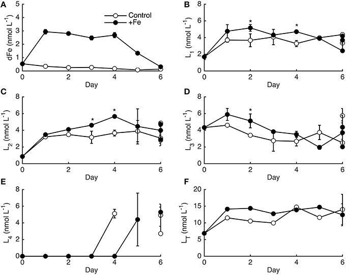
Figure 4. The dFe (A) and ligand data (B–F) for incubation experiment 1 in controls (open circles) and +Fe (closed circles) treatments. Error bars represent the standard deviation between the two linearization techniques employed, except on day 6 where error bars represent the standard deviation between replicate bottles. The * indicates a significant difference in ligand concentrations on that day when the standard deviation between replicate bottles observed on day 6 are considered (t-test, p < 0.05).

Incubation Experiment 2

Experiment 2 was conducted in the dark for 3 days following the termination of experiment 1 on day 6. Control and +Fe bottles initially contained different amounts of phytoplankton biomass (Figure 3B), but relatively similar dFe and ligand concentrations (Figure 5A). The goal of this experiment was to assess microbial alteration of the ligand pool in response to distinct amounts of particulate biomass and Fe. Control bottles contained 0.14 ± 0.05 nmol L⁻¹ dFe (n = 3) on day 1 of the experiment, and by day 3, 0.54 ± 0.33 nmol L⁻¹ dFe had been remineralized (n = 3). In +Fe treatments the dFe increased from 0.31 ± 0.07 nmol L⁻¹ (n = 3) on day 1 to 1.29 ± 0.21 nmol L⁻¹ (n = 3) on day 3. In general, ligands increased more in the controls than in the +Fe treatments (Figure 5A), though there was high variability between replicate bottles. L₁ ligands increased by 32.6 ± 1.7% on average in controls (n = 3), but they decreased by 1.3 ± 1.2% in +Fe bottles (n = 3; Figure 5B). A similar pattern was seen for L₂ ligands, which increased by 29.7 ± 2.1% in control treatments, but decreased by 16.8 ± 2.0% in +Fe bottles (n = 3). L₃ ligands decreased in both treatments, but by a significantly higher percentage (t-test, p < 0.05) in controls (33.9 ± 2.1%) than in the +Fe case (5.9 ± 2.5%). The weakest ligands (L₄) showed the greatest change between days 1 and 3 in both treatments, but increased by a significantly (t-test, p < 0.05) greater percentage in controls (109.1 ± 3.2%) compared to +Fe bottles (32.8 ± 4.9%, n = 3). In general, the average concentration of total ligands (L₁+L₂+L₃+L₄) was higher in controls on day 3 than in +Fe bottles on day 3 (t-test, p < 0.05).

FIGURE 5

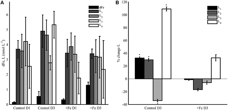
Figure 5. (A) The dFe (black bars), L₁ (dark gray bars), L₂ (gray bars), L₃ (light gray bars), and L₄ (white bars) ligand concentrations from incubation experiment 2 in controls (left) and +Fe treatments (right) on day 1 (D1) and day 3 (D3). Error bars represent the standard deviation from replicate bottles for the control (A, B, C) and +Fe (FeA, FeB, FeC) treatments. (B) Average percent change in ligand concentrations from day 1 to 3, where * indicates a significance difference in the percent change in ligand concentrations from day 1 (t-test, p < 0.05).

Modeling of Incubation Experiment 1

Numerical experiments were performed for incubation experiment 1 in order to investigate biological ligand sources and sinks based on non-measured parameters (e.g., bacterial growth rate and abundance). As part of the CCE-LTER program, other ancillary data including some rate measurements were obtained at the same station and depth for experiment 1 (station 3) and were used as the initial values of key parameters in the model, with some adjustments (Table 1). Changes in nutrient concentrations over time both in control and +Fe treatments (Figures 6A–C) and the increase in chl a (Figure 6D) were all reasonably reproduced by the model. No measurements were made for bacterial abundance or organic matter concentrations during the course of experiment 1, but the model results show an increase in both bacteria and particulate organic nitrogen (PON) in +Fe treatments (Figures 6E,F). The temporal patterns in L₁ and L₂ were also described relatively well, with the exception of day 6, where the model shows greater separation between controls and +Fe bottles (Figures 6G, H). Initial ligand production in the model (days 0–2) is due to rapid ligand production in both treatments from residual Fe stress of the initial water mass (expressed as bacteria stress in the model), and constant photochemical degradation in both treatments. Lower rates of ligand production in later days of the incubation are because of higher ligand degradation rates (proportional to ligand concentrations) and lower bacteria biomass in the control case, as expressed in the model. The differences between treatments in the model become apparent between days 4 and 6, owing to larger differences in bacteria biomass and organic matter in +Fe treatments (Figures 6E,G) and ligand production from PON (e.g., Boyd et al., 2010).

FIGURE 6

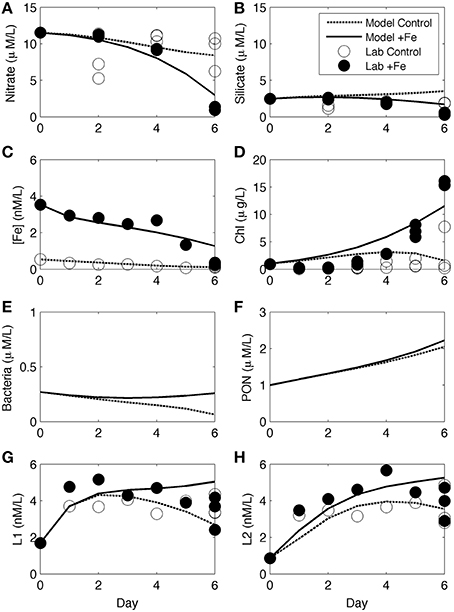
Figure 6. Numerical modeling results from incubation experiment 1. Results for nitrate (A), silicate (B), [dFe] (C), chl a (D), bacteria abundance (E), PON (F), L₁ (G), and L₂ (H) are shown from the model of the controls (dashed line) and +Fe treatments (dark line), along with the data from controls (open circles) and +Fe treatments (closed circles).

Photochemical Experiments

Each photochemical experiment was completed using water collected from the chl a maximum at each station (30 m for station 1, 70 m for station 2, and 20 m for station 6). The first experiment at station 1 contained similar concentrations of strong ligands in the initial condition and dark treatments, and slightly higher [L₂] were observed in the light treatment (Figure 7A), though the differences were not significant (t-test, p > 0.05). No weaker ligands (L₃) were observed in this experiment in the initial or final conditions. Experiments 2 and 3 from stations 2 and 6, respectively, showed different results (Figures 7B,C). Again, the dark bottles contained similar [dFe] and ligands as initial conditions in both experiments, but light treatments had lower concentrations of L₁ ligands and also contained L₃ ligands, which were absent initially and in the dark treatments (Figures 7B,C). The weakest ligands measured in this study (L₄ ligands) were not detected in any of the photochemical experiments.

FIGURE 7

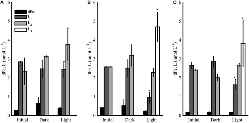
Figure 7. The dFe (black bars) and ligand concentrations (L₁-L₃) for photochemical experiments 1 (A), 2 (B), and 3 (C) in the initial and final conditions after 12 h (Dark and Light). Error bars represent the standard deviation between replicate bottles in dark (A, B) and light (A, B) bottles, and * represents a significance difference in ligand concentrations from initial conditions (t-test, p < 0.05).

Discussion

Distribution of Multiple Classes of Iron-Binding Ligands in the Southern California Current System

The dFe and ligand profiles in this study were similar to those measured in other oceanic regimes (see Gledhill and Buck, 2012), with a minimum in ligands in surface waters and an increase with depth along with dFe and nitrate (Figure 2). Ligand profiles between stations were also similar, despite the differences in biogeochemical regimes sampled (Krause et al., 2015). Most of the profiles had a surface minimum in L₁ ligands (Figure 2), perhaps related to photochemical degradation, consistent with previous findings in surface waters (see Gledhill and Buck, 2012). This feature can be patchy however, since station 6 for example, had a maximum in L₁ at the shallowest depth sampled (20m, Figure 2F). The minimum in L₁ was also sometimes associated with elevated concentrations of L₃ in the profiles, though not at station 1. There appear to be other dynamics affecting [L₁] in the profiles as well, as a maximum in L₁ can be seen at stations 2 and 6 associated with, or near, the chl a maximum (Figure 2). Other studies have also observed a maximum in strong ligands associated with the biomass maximum (Rue and Bruland, 1995; van den Berg, 1995, 2006; Boye et al., 2001, 2005; Croot et al., 2004; Gerringa et al., 2006, 2008; Buck and Bruland, 2007; Wagener et al., 2008; Ibisanmi et al., 2011). The mechanism leading to this feature is not entirely clear, but one field study done in the Canary Basin showed that 63% of the variance in ligands above, or coinciding with, the chl a maximum was explained by phytoplankton biomass and silicic acid concentrations (Gerringa et al., 2006). In this study, L₁ was defined as any ligands with a log $K_{F e L_{1}, F e^{'}}^{c o n d} \geq$ 12.0, and were present at all depths sampled (up to 500 m). In our previous work examining surface samples in the central and northern CCE we also found that L₁ declined in surface waters offshore (>200 km), perhaps due to degradation of the stronger ligand class, or a nearshore source, though only a few samples were measured offshore (Bundy et al., 2014b). Other studies have also noted a slight decline in ligand strength from coastal to offshore waters (Sander et al., 2014). All stations sampled in this region were within 200 km off the coast (Figure 1), and L₁ was present in surface waters of each station (Figure 2). Thus, it is still uncertain whether L₁ is restricted to within 200 km of the coast in this region. On a GEOTRACES zonal transect in the Atlantic however, recent work has shown L₁-type ligands (average log $K_{F e L_{1}, F e^{'}}^{c o n d}$ = 12.38 ± 0.22, n = 476) throughout the entire water column, down to 6000 m (Buck et al., 2015). There is likely an in-situ source of strong ligands throughout the water column, or the residence time of strong ligands is longer than dFe (Gerringa et al., 2015).

L₂ distributions were very similar to the distributions of L₁ in the profiles (Figure 2). L₂ ligands, as defined in this study, are generally still considered “strong” in terms of previous work on dFe-binding ligands (Gledhill and Buck, 2012), and thus may be controlled by similar processes as L₁. Our other work in coastal regions has also demonstrated a strong coupling between these two ligand classes (Bundy et al., 2014a,b). From the bulk of previous studies measuring dFe-binding ligands, L₂ appears to be a relatively ubiquitous ligand class even in deeper waters (Gledhill and Buck, 2012). Buck et al. (2015) also measured an L₂ ligand class on the zonal Atlantic GEOTRACES transect (log $K_{F e L_{2}, F e^{'}}^{c o n d}$ = 11.46 ± 0.27, n = 450) which was also present down to 6000 m along with L₁. Thus, similar processes may affect the cycling of L₁ and L₂ in the water column.

The distributions of the weaker ligands detected in the profiles (L₃) were somewhat distinct from the stronger ligands. L₃ concentrations were almost constant with depth at most stations, with a slight minimum in surface waters at station 1 (Figure 2). Evidence from our previous work has shown that L₃ ligands increase in surface samples in a transect from nearshore to offshore in the CCS (Bundy et al., 2014b), possibly due to degradation of L₁ and L₂. Elevated concentrations of L₃ in the profiles relative to stronger ligands support this preliminary hypothesis. The slight minimum in surface waters might be related to dissolved organic matter (DOC) uptake, if L₃ ligands comprise a portion of the labile organic matter pool utilized by bacteria. The hypothesis that microbial communities are responsible for altering the weaker ligand pool in the deep ocean (Hunter and Boyd, 2007; Boyd et al., 2010) is also supported by the results from the water column profiles, suggesting an in-situ source of weaker ligands in subsurface waters. Buck et al. (2015) also measured an L₃ ligand class (log $K_{F e L_{3}, F e^{'}}^{c o n d} = 10$ .84 ± 0.14, n = 54) detectable in subsurface waters, though less often than L₁ and L₂.

Iron-Binding Ligand Dynamics in Biological Incubation Studies

Two experiments were performed in this study in order to observe the temporal evolution of the ligand pool during phytoplankton growth (incubation experiment 1) and microbial remineralization of particles (incubation experiment 2). Each experiment revealed different possible mechanisms leading to alteration of the ligand pool over time. Incubation experiment 1 examined changes in dFe-binding ligands associated with an Fe-addition grow-out (Figure 4). Although there have been links between diatom growth and changes to the ligand pool observed in previous incubation studies (Buck et al., 2010; King et al., 2012), incubation experiment 1 showed somewhat different results. Likely, some of these differences were related to the characteristics of the initial water mass. For example, experiment 1 was initiated under Fe-limiting conditions, as evidenced by the initial NO₃⁻:dFe (Figure 3C) and the eventual diatom response to Fe addition (Figure 3B). Experiment 1 also initially had elevated strong ligand concentrations, which continued to increase for the first few days of the experiment and then remained relatively constant after day 3 (Figure 4). It is possible that the high concentrations of strong ligands in experiment 1 remained elevated over time due to initial Fe-limitation of the planktonic community, in contrast to other incubation studies which were initiated in nutrient replete waters and evolved into Fe-limitation over the course of the incubation (Buck et al., 2010; King et al., 2012). This was corroborated by the modeling experiment, where the model could reasonably reproduce the initial increase in strong ligands from days 0 to 3 if the bacteria were Fe-stressed (Table 1). Another possibility is that these ligands continue to be produced, but are cycled over short timescales.

Overall, the difference in phytoplankton biomass in experiment 1 between controls and +Fe bottles was striking, yet the temporal ligand patterns were relatively similar. These results suggest that phytoplankton growth did not have a strong effect on the ligand concentrations observed. Bacteria were not directly sampled in incubation experiment 1 due to volume constraints, but the potential effect of nutrient limitation on bacteria growth was analyzed via modeling (Figure 6). Modeling results were able to depict the cycling of the stronger ligand pool (L₁ and L₂) reasonably well with only bacteria as the biological source of ligands (Figure 6). In this model, L₁ is assumed to be solely from bacteria, while L₂ is assumed to be the product of PON degradation (Boyd et al., 2010) and photochemical degradation of L₁. In the current case, we assumed the bacteria were at their maximum ligand productivity in both control and +Fe treatments due to the Fe-limited status of the initial water mass, so there was no difference in L₁ production between the two treatments. This was to explain the rapid L₁ increase in the first 2 days under both +Fe conditions (Fe replete) and controls (Fe deficient; Figure 4). With these assumptions, modeled L₁ and L₂ concentrations agree with the data reasonably well in both treatments. In the model, continual L₁ production occurs in controls due to Fe stress, and L₂ is primarily produced from photochemical degradation during days 0–2. During days 2–4, L₂ concentrations show more disparity between the two treatments, likely due to the combination of more L₁ and L₂ being produced in the +Fe treatment, due to higher bacterial abundance and more PON, respectively. Phytoplankton biomass began to increase in +Fe treatments after day 3, which translates into a larger increase in PON (Figure 6F) and more bacteria. It is this elevated PON and bacteria that lead to the difference in accumulated ligands, but the model yields larger differences in ligand concentrations on day 6 than was observed. It is possible that the model over-estimates bacteria biomass differences between treatments during the latter stages of the experiment, or other parameters not accounted for in the model are responsible for the trends observed. The average of all three triplicates of each treatment does not yield a significant difference between controls and +Fe bottles on day 6 (t-test, p > 0.05), and the differences between controls and +Fe bottles in terms of L₁ and L₂ distribution were minimal over the time course of the incubation, suggesting the evolution of Fe-stress in the treatments may not have been a major factor in ligand production. The model is able to replicate the observed ligand distributions relatively well by simply invoking two different biological mechanisms for strong ligand production—production of L₁ under Fe stress, and production of ligands associated with degradation of PON (L₂). Strong ligand production is generally understood to be an Fe acquisition strategy when Fe is scarce (Granger and Price, 1999). However, there is mounting evidence that bacteria also produce siderophores when macronutrients and/or Fe are replete (Gledhill et al., 2004; Mawji et al., 2011; Adly et al., 2015). Our results suggest that strong ligands can be modeled relatively well with only bacteria as a biological source of ligands under both Fe replete and Fe deficient conditions, though many other factors are likely to influence the temporal patterns observed.

We did not attempt to model the weaker ligands in incubation experiment 1, but several studies have shown a link between dFe-binding ligand production and diatom growth (Trick et al., 1983; Soria-Dengg et al., 2001; Gerringa et al., 2006; Rijkenberg et al., 2008; Buck et al., 2010; King et al., 2012). Chaetoceros brevis has been observed to alter the ligand pool in culture media (Rijkenberg et al., 2008; González et al., 2014), and was one of the dominant diatom species in experiment 1 (in both control and +Fe treatments). Other evidence from the field has shown that ligands are produced associated with large diatom blooms such as those observed during Ironex-II (Rue and Bruland, 1997) and SEEDS II (Kondo et al., 2008). Phytoplankton have also been shown to release polysaccharides and other cellular material during growth (Watt, 1969; Myklestad et al., 1989; Urbani et al., 2005), which may explain the increase in weaker ligands observed on days 4–6 in experiment 1 (Figure 4D). It is not entirely certain what compounds may comprise the weaker ligand pool in the marine environment, but the decrease in the L₃ ligand class over the duration of experiment 1 along with a slight increase at the termination of the experiment points to perhaps polysaccharides or some other form of relatively labile DOC (Ducklow et al., 1993). Polysaccharides would likely fall into the L₃ ligand category in this study (Hassler et al., 2011; Norman et al., 2015), and are readily consumed by most bacteria as a source of DOC (Zweifel et al., 1993; Arnosti et al., 1994). The L₄ ligand class was only detected on days 4–6 in experiment 1 (Figure 4E) and could be partially explained by the release of domoic acid by Pseudo-nitzschia, which are known to produce this compound during bloom formation (Rue and Bruland, 2001). Domoic acid has a log $K_{F e L, F e^{'}}^{c o n d} =$ 8.6, which falls into the L₄ class as defined in this study (Rue and Bruland, 2001). These ligands may have also been comprised of other degraded cellular material, such as viral lysis products (Poorvin et al., 2011), or other high molecular weight (HMW) compounds that have been shown to effectively bind dFe (Laglera and van den Berg, 2009; Abdulla et al., 2010). HMW compounds have also been identified in association with diatom growth in culture media containing T. weiss and C. antigua (Fuse et al., 1993), suggesting other diatoms in experiment 1 may have contributed to the increase in the weaker ligand pool at the end of experiment 1 (Rijkenberg et al., 2008).

While diatoms were potentially responsible for changes in the ligand pool in incubation experiment 1, the production of dFe-binding ligands has also been associated with copepod grazing (Sato et al., 2007). Grazing could be one of the reasons for the initial increase in stronger ligands from day 0 to 1 (Figures 4B,C), though no copepods were evident in the incubation bottles. Grazing may also be an explanation for higher [L₂] on days 3–5 in +Fe treatments in experiment 1 (Figure 4C), coinciding with elevated diatom growth on those days. However, due to similarities between controls and +Fe bottles in experiment 1, it is unlikely that phytoplankton grazing was a significant factor affecting ligand concentrations in that experiment. This hypothesis is corroborated by the modeling results for Experiment 1, which show there were potentially significant differences in grazing rates between controls and +Fe treatments during the later days of the experiments (data not shown). This implies there should be differences in ligand concentrations between treatments if zooplankton grazing was a significant source of ligands, but this was not observed.

The temporal pattern in ligands in incubation experiment 1 was likely the result of several processes, perhaps dominated by bacteria. The ability for the heterotrophic community to alter the ligand pool was explicitly tested in incubation experiment 2 (Figure 5). Microbial remineralization of organic particles has been examined previously by Boyd et al. (2010) in the Southern Ocean, who found that microbial breakdown of POC produced dFe and L₂ ligands (Boyd et al., 2010). Our incubation study examined microbial remineralization of several ligand classes using MAWs, and found that almost all the ligand classes increased significantly over the incubation period in controls (days 1–3) and the overall ligand increase was greater in controls than +Fe treatments. It is possible the strong ligands produced during experiment 2 could be siderophores, especially in control treatments that contained very low [dFe] even after some had been remineralized (Figure 5). L₃ ligands demonstrated a different pattern than the other ligand classes in Experiment 2, since they decreased slightly from day 1 to 3, though the differences between the initial and final time points were not significant in either treatment (t-test, p > 0.05). Similar to experiment 1, it is possible that some form of labile DOC falls into the L₃ ligand category, which may have been consumed during this experiment. In contrast to L₃, L₄ clearly increased during experiment 2. This is consistent with other observations that have shown that HMW organic compounds, likely with weak dFe-binding, can increase due to DOC remineralization (Repeta et al., 2002).

Iron-Binding Ligand Dynamics in Photochemical Studies

Photochemical experiments from this region showed mixed results with respect to the effect of natural sunlight on the dFe-binding ligand pool (Figure 7). This is similar to other field efforts, where some studies have observed a decrease in the concentration of strong dFe-binding ligands upon exposure to natural sunlight (Powell and Wilson-Finelli, 2003) and others have seen no effect of UV light on ligands found in Dutch estuaries (Rijkenberg et al., 2006). Thus, it appears not all natural dFe-binding ligands are susceptible to photo-degradation, as has been shown with certain siderophores in laboratory studies (Barbeau et al., 2001, 2003; Barbeau, 2006). One reason for this difference in reactivity may be related to the size class, functional groups, or binding strength of the natural ligands present in the environment. Some of the natural dFe-binding ligands found by Powell and Wilson-Finelli (2003) had slightly elevated log $K_{F e L, F e^{'}}^{c o n d}$ compared to the Rijkenberg et al. (2006) study (log $K_{F e L, F e^{'}}^{c o n d}$ ~12 compared to 10.1–11.0), and no degradation of the strong ligands was observed by Rijkenberg et al. (2006). L₁ ligands observed initially in photochemical experiment 1 were slightly weaker (log $K_{F e L, F e^{'}}^{c o n d} = 12.51$ ± 0.14), though still strong, than in experiments 2 and 3 (13.70 ± 0.02 and 12.79 ± 0.15, respectively; t-test, p < 0.05), though this difference is not striking. The differences in photochemical reactivity between experiments is most likely the result of distinctions in the initial water mass. It is notable that no L₃ ligands were detected initially in any of the photochemical experiments, despite the fact that L₃ ligands were detected in the water column at similar depths (Figure 2). We speculate that there was some scavenging of L₃ ligands onto the walls of the quartz flasks used in this study, since the initial samples were taken directly from the flasks after filling and we have noted this problem in other experiments with quartz (data not shown). This may be another reason for differences in field studies examining degradation of natural ligands, if weaker ligands produced from photo-degradation are rapidly scavenged.

Another possible explanation for mixed findings in earlier publications may be related to analytical methods. This study employed MAW analysis, which enabled the detection of both the strongest and weakest dFe-binding ligands (α_{Fe(SA)_x} = 74−115). Powell and Wilson-Finelli (2003) employed a low (α_Fe(TAC)₂ = 55) and high (α_Fe(TAC)₂ = 300) analytical window, while Rijkenberg et al. (2006) used only a high window (α_Fe(TAC)₂ = 300). It is possible that the competition strength in the Rijkenberg et al. (2006) study may have been too high to effectively detect some of the weaker dFe-binding ligands. These differences in analytical methods support the utility of using MAWs in the context of mechanistic ligand studies where more than one class of dFe-binding ligand may be detected.

Processes Affecting Iron-Binding Ligands in the Southern California Current System

To our knowledge, this is the first study to mechanistically link dFe-binding ligand profiles with deckboard incubation experiments on the same cruise, using MAW analysis of the ligand pool. Although only a few profiles were examined in this study, the stations were in biogeochemically distinct sampling regions and large hydrographic and biological gradients were also sampled vertically. Despite the relatively large gradients, the ligand profiles were very similar between stations. Coastal station 4, for example, had much higher [chl a] in the subsurface maximum, but did not show a difference in ligands at this depth compared to any other station (Figure 2). Similarly, incubation experiment 1 showed very little difference in the ligand pool between the Fe-limited vs. the Fe-replete phytoplankton community (Figure 4), despite the much higher biomass in +Fe bottles (Figure 3B). These findings suggest that large changes in phytoplankton biomass in surface waters may have little impact on the overall composition of the Fe-binding ligand pool on longer timescales.

MAW analysis helped to reveal the presence of three ligand classes at almost every sampling depth in the upper 500 m of the southern CCS, suggesting there are ubiquitous in-situ sources of each of these ligand classes, or they have a relatively long residence time. Although no other studies have used MAWs to measure dFe-binding ligand profiles, most recent studies agree that both strong and weak ligands are present throughout the water column (Buck et al., 2015; Gerringa et al., 2015). Experimental and statistical evidence from this study suggests a mechanism for the presence of both strong and weak ligands in surface and subsurface waters. The patterns in the ligand distributions between profiles were primarily correlated with nitrate distributions, which could point to microbial remineralization as a potentially dominant control on the ligand pool with depth over longer timescales (Gerringa et al., 2015). A field study also found a close link between ligand concentrations in surface waters, DOC and bacterial abundance (Wagener et al., 2008) and bacteria are known to be the dominant control on DOC in the ocean. Although some interesting features were also seen in the upper water column that may be related to phytoplankton dynamics, these processes may occur on shorter timescales than microbial remineralization processes. Incubation experiment 2, which focused on the ability of the heterotrophic community to produce dFe-binding ligands from POC remineralization, showed that strong ligands can be produced during this process, in addition to the weaker ligands observed in Boyd et al. (2010). The results from incubation experiment 2 now provide a mechanism for in-situ strong ligand production in subsurface waters as well.

Although L₄ ligands appeared to be produced during both biological incubation experiments, none were detected in the profiles (Figure 2). It may be that these weaker dFe-ligand complexes are scavenged on longer timescales and were therefore not present in the station data, or that L₄ ligands have only a nearshore source such as the benthic boundary layer or coastal estuaries as seen in our previous work (Bundy et al., 2014a,b). L₄ ligands may only be present under certain conditions or on certain timescales in the oceanic water column. The biological incubation experiments performed in this study suggest that there are, however, in-situ sources for these very weak ligands in the oceanic environment.

Subsurface ligand concentrations could be largely controlled by the microbial community, but photochemical effects appear to impact near surface waters in this region as well. Evidence from photochemical experiments suggests that photochemical degradation of natural ligands can be variable, and may be restricted to the strongest or certain size classes of ligands. This may provide an explanation for regional differences between studies on photochemical effects (Powell and Wilson-Finelli, 2003; Rijkenberg et al., 2006) and the differences between stations in this study (Figure 2). Additional explanations for the variable influence of photochemistry on the natural ligand pool will be important to constrain in future studies, as it appears to be a significant sink for L₁ in CCE surface waters.

Author Contributions

RB and KB both contributed to the design of the experiments and the acquisition and interpretation of the ligand and nutrient data. MC analyzed, processed and interpreted the cell count data. MJ developed and tested the incubation experiment model. RB, MC, KB, and MJ critically revised the work for intellectual content and ensured the integrity of the reported data.

Conflict of Interest Statement

The authors declare that the research was conducted in the absence of any commercial or financial relationships that could be construed as a potential conflict of interest.

Acknowledgments

We would like to thank the captain and crew of the R/V Melville and the CCE-LTER program. We would like to thank Teresa Fukuda for phytoplankton pigment measurements. We also thank Wendy Plante and Shane Hogle for help with sampling. RB, KB, and MC were supported by NSF OCE #10-2667 for the CCE-LTER program. MJ was funded by NSF ANT grant 0948378 and Harbor Branch Oceanographic Institute Foundation.

Supplementary Material

The Supplementary Material for this article can be found online at: https://www.frontiersin.org/article/10.3389/fmars.2016.00027

Abbreviations

CCS, California Current System; Chl a, chlorophyll a; CLE-ACSV, competitive ligand exchange-adsorptive cathodic stripping voltammetry; CSV, cathodic stripping voltammetry; CTD, conductivity, temperature, and depth sensor; dFe, dissolved Fe; DOC, dissolved organic carbon; DOM, dissolved organic matter; Fe, iron; FPE, fluorinated polyethylene; GF/F, glass fiber filter; HCl, hydrochloric acid; HMW, high molecular weight; HNLC, high nutrient low chlorophyll; HPLC, high performance liquid chromatography; LDPE, low density polyethylene; LTER, Long Term Ecological Research; L_x, an iron binding ligand class, where x denotes ligand class (1–4); MAWs, multiple analytical windows; MilliQ, purified water; POC, particulate organic carbon; PON, particulate organic nitrogen; S, salinity; S_IN, internal sensitivity; SA, salicylaldoxime; SAFe, Sampling and Analysis of iron (Fe); UV light, ultra-violet light.

References

Abdulla, H. A. N., Minor, E. C., Dias, R. F., and Hatcher, P. G. (2010). Changes in the compound classes of dissolved organic matter along an estuarine transect: a study using FTIR and C-13 NMR. Geochim. Cosmochim. Acta 74, 3815–3838. doi: 10.1016/j.gca.2010.04.006

ORIGINAL RESEARCH article

Iron-Binding Ligands in the Southern California Current System: Mechanistic Studies

Introduction

Methods

Sampling Region and Environmental Context

Sampling and Storage

Nutrients and Phytoplankton

Dissolved Iron

Dissolved Iron-Binding Ligands

Experimental Set-Up

Biological Incubation Experiments

Photochemical Experiments

Modeling

Statistical Analyses

Results

Water Column Profiles

Biological Ligand Production Experiments

Incubation Experiment 1

Incubation Experiment 2

Modeling of Incubation Experiment 1

Photochemical Experiments

Discussion

Distribution of Multiple Classes of Iron-Binding Ligands in the Southern California Current System

Iron-Binding Ligand Dynamics in Biological Incubation Studies

Iron-Binding Ligand Dynamics in Photochemical Studies

Processes Affecting Iron-Binding Ligands in the Southern California Current System

Author Contributions

Conflict of Interest Statement

Acknowledgments

Supplementary Material

Abbreviations

References

This article is part of the Research Topic

People also looked at