Impact of El Niño Variability on Oceanic Phytoplankton

Introduction

Phytoplankton, the microscopic vegetal cells living at the surface of the oceans, yield globally and annually some fifty billion tons of organic carbon through primary production (Longhurst et al., 1995), contributing to the oceanic uptake of ~25% of the carbon dioxide (CO₂) emitted to the atmosphere every year (Le Quéré et al., 2015). The rates of primary production are not uniformly distributed across the ocean domain: the most highly productive oceanic regions are found at high-latitudes and in coastal upwelling systems. Oceanic primary producers are under the control of physical forcing on a broad spectrum of scales, and the forcing will be modified under climate change. In the latest assessment report (AR5), the Intergovernmental Panel on Climate Change (IPCC) has recognized “medium evidence” for the response of the highly productive oceanic regions to recent warming (especially since the 1970s) and “low confidence” in the understanding of how equatorial upwelling systems might change in response to El Niño variability (Hoegh-Guldberg et al., 2014).

El Niño activity is characterized by anomalous warming of Sea Surface Temperature (SST) in the tropical Pacific, linked to a perturbation of atmospheric circulation patterns known as the Southern Oscillation. This ocean-atmosphere coupling, called the El Niño Southern Oscillation (ENSO), is a dominant mode of variability in the Earth-climate system with a typical frequency of 2–7 years (McPhaden et al., 2006; Cai et al., 2015). Each El Niño event is unique, exhibiting differences in surface and subsurface water temperature amplitude, duration, and spatial patterns (Capotondi et al., 2015). As an aid to classify El Niño events, the location of maximum anomalous SST warming observed during boreal winter has been used to delineate two extreme types of El Niño (Trenberth and Stepaniak, 2001; Larkin and Harrison, 2005; Ashok et al., 2007; Yu and Kao, 2007; Ashok and Yamagata, 2009; Kao and Yu, 2009; Kug et al., 2009; Lee and McPhaden, 2010; Takahashi et al., 2011; Cai et al., 2015; Capotondi et al., 2015). The Eastern-Pacific (EP) El Niño, also referred to as the “typical” or canonical El Niño, is characterized by maximum anomalous SST warming in the eastern tropical Pacific. In contrast, the Central-Pacific (CP) El Niño, variously referred to as El Niño Modoki (a Japanese word meaning pseudo), warm-pool El Niño, or dateline El Niño, is characterized by weak anomalous SST warming along the western coast of South America and maximum anomalous SST warming in the central tropical Pacific. The climatic perturbations generated by these two types of El Niño are induced through different atmospheric teleconnections: both have been associated with changes in temperature and rainfall patterns over the continental U.S. (Yu et al., 2012; Yu and Zou, 2013), in storm tracks in the Southern Hemisphere (Kao and Yu, 2009) and in cyclone trajectories in the North Atlantic (Kim et al., 2009). Since the beginning of the 1900s, two most extreme EP and CP El Niño events (in terms of amplitude of maximum SST anomalies in the Eastern and Central Pacific regions) have occurred within the last 20 years, in 1997/1998 and 2009/2010 respectively (Capotondi et al., 2015). The latest 2015/2016 El Niño has been reported with comparable magnitude of SST anomalies to the 1982/1983 and 1997/1998 events but with more limited intensity in the Eastern Pacific region (Paek et al., 2017; L'Heureux et al., in press).

Contrasting influence of the extreme El Niño events of 1997/1998 and 2009/2010 on oceanic phytoplankton has been characterized in the tropical Pacific domain (Gierach et al., 2012; Radenac et al., 2012). In this region, ENSO is recognized as the main driver of inter-annual phytoplankton variability. Tropical, as well as extra-tropical, influences of ENSO and ENSO Modoki have been demonstrated using statistical analyses based on a range of indices applied to ocean-color remote-sensing observations (Yoder and Kennelly, 2003; Behrenfeld et al., 2006; Chavez et al., 2011; Vantrepotte and Mélin, 2011; Messié and Chavez, 2012, 2013; Racault et al., 2012, 2017; Couto et al., 2013; Raitsos et al., 2015). One of the most widely-used environmental indices to characterize influence of ENSO on ocean biology is the Multivariate ENSO Index (MEI). This index is based on combined analysis of fields of sea level pressure, surface winds, SST, surface air temperature, and cloudiness for the entire Tropical Pacific domain (Wolter and Timlin, 1993). Due to this broad domain and multivariate statistical approach, the MEI encompasses the whole continuum of ENSO events (from most extreme SST anomalies located in the Central to Eastern Pacific regions), but as a result, the index does not allow us to separate effects of EP and CP El Niño variations. Separating EP and CP El Niño variations requires indices isolating the centroid of El Niño activity along the equatorial Pacific.

To date, the longitudinal position of the center of maximum SST anomalies has been delineated in the Niño1+2 (0°–10°S, 90°–80°W), Niño3 (5°–5°N, 150°W–90°W), Niño3.4 (5°N–5°S, 170°W–120°W) and Niño4 (5°–5°N, 160°E–150°W) regions (Ashok et al., 2007). Based on analyses of the SST anomalies variations in these regions, a range of El Niño indices have been constructed. In the present study, the EP and CP El Niño signals are characterized using the EP and CP index defined by Kao and Yu (2009). The EP index was calculated by first applying regression analysis of SST anomalies onto the Niño4 index (average SST anomalies over the Niño4 region) to remove the influence of the SST anomaly component associated with central Pacific warming, and then using Empirical Orthogonal Function (EOF) analysis to determine the spatial patterns and associated temporal index of EP events. Similarly, the CP index was calculated by applying regression analysis of SST anomalies onto the Niño1+2 index to remove the influence of the SST anomaly component associated with east Pacific warming, and then using EOF analysis to characterize pattern and index of CP events (Kao and Yu, 2009; Yu et al., 2012). Using partial correlation and EOF analyses, the characterization of the canonical El Niño and El Niño Modoki signals has also been achieved based on SST anomalies from the Niño3 region and by differentiating the influence of SST anomalies variations from a combination of regions in the tropical Pacific. The specific combination and definition of regions have been formulated as the Trans-Nino Index TNI (Trenberth and Stepaniak, 2001), the El Niño Modoki Index EMI (Ashok et al., 2007), and the Improved EMI (Li et al., 2010). A comprehensive review of El Niño indices definition is presented by Capotondi et al. (2015).

The main obstacles to distinguishing the ecosystem effects associated with El Niño variability may be summarized to arise from: (i) the challenges to construct continuous, synoptic-scale, long-term time-series of marine ecosystem state at high temporal and spatial resolutions for the global oceans (Sathyendranath and Krasemann, 2014); (ii) the diversity and complexity of the mechanisms driving the biophysical interactions in different oceanic sub-regions or provinces (Longhurst et al., 1995; Boyd et al., 2014); (iii) the difficulties to elucidate the roles of the local and remote-forcing mechanisms associated with different El Niño events (Cai et al., 2015; Capotondi et al., 2015); (iv) the issues of lag in the transmission of El Niños influences at higher latitudes and to other basins via different teleconnection mechanisms (Ashok et al., 2007; Couto et al., 2013); and finally (v) the broad ranges of meridional position, amplitude and evolution of SST anomalies observed during different El Niño events, which militate against consensus in the choice of method to estimate indices of El Niño variability (Capotondi et al., 2015). Here, we propose an original approach that overcome some of these obstacles based on climate-quality ocean-color products and state-of-the-art reanalysis datasets, and allow us to establish an atlas of the impact of CP and EP types of El Niño on primary producers in the global oceans. Finally, we document the associated environmental changes and identify the dominant mechanisms driving the diverse biophysical interactions involved.

Materials and Methods

The list of biological and physical datasets obtained for the analyses is summarized in Table 1. Based on datasets availability, two periods of study have been considered: (1) 1997–2012 (15 years) for biological and physical datasets, and (2) 1979–2014 (35 years) for physical datasets only.

TABLE 1

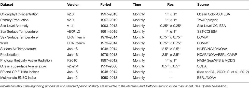
Table 1. Datasets obtained for the analysis.

Biological Datasets

Remotely-Sensed Chlorophyll Concentration and Associated Uncertainty Estimates

Chlorophyll is at the heart of primary production, it is the state variable used in photosynthesis-irradiance models to compute primary production; it has a distinct optical signature which makes it one of the easiest phytoplankton properties to measure, both by in-situ and satellite methods. Ocean-color sensors on satellites provide estimates of chlorophyll concentration at high spatial and temporal resolution and at global scale. Because they provide data consistently and frequently and over long periods of time, they are suitable for computations of certain ecological indicators and for studying long-term trends in the state of the marine ecosystem (Platt and Sathyendranath, 2008; Racault et al., 2014). However, ocean-color sensors do have a finite lifespan, and differences in instrument design and algorithms make it difficult to compare data from multiple sensors. When overlapping data are available from two or more sensors, such data can be used to establish inter-sensor bias and correct for it. Recently, under the European Space Agency (ESA) Climate Change Initiative (CCI), the ocean-color project (http://www.esa-oceancolour-cci.org) has produced new, improved products, merging observations from the Sea-viewing Wide Field-of-View Sensor (SeaWiFS, 1997–2010), the Moderate Resolution Imaging Spectroradiometer (MODIS, 2002-present) and the MEdium Resolution Imaging Spectrometer (MERIS, 2002–2012) to provide a 15-year (1997–2012 OC-CCIv2) global scale, climate-quality controlled, bias-corrected, and error-characterized data record of ocean-color (Sathyendranath and Krasemann, 2014). Furthermore, implementation of the coupled ocean-atmosphere POLYMER correction algorithm (MERIS period; Steinmetz et al., 2011) has increased significantly the coverage of chlorophyll observations (Sathyendranath and Krasemann, 2014; Racault et al., 2015).

The OC-CCI v2.0 Level 3 Mapped data of chlorophyll concentration, root-mean-square-difference (RMSD) and bias estimates of monthly log-transformed (base 10) Chl, were obtained at 4 km spatial resolution, and monthly temporal resolution from the ESA CCI Ocean Color website at http://www.esa-oceancolour-cci.org. To remain coherent with the resolution of the different datasets used in the analyses (Table 1), the chlorophyll concentration was mapped onto a 1° × 1° regular grid by averaging all available data points within each new, larger pixel. Standard deviation of chlorophyll product (computed from bias and RMSD) was calculated by aggregating pixel values at the same spatial (1° × 1°) resolution. Then, the standard deviation of the log10Chl was converted to its untransformed value. The standard error in the reported mean value at each pixel for the period 1997–2012 was computed, and values ranging between ±1% in the tropical gyres (associated with low chlorophyll concentration) and below ±0.5% at higher latitudes (associated with high chlorophyll concentration) were observed (Supplementary Figure 1). Uncertainties in the anomalies of relative (%) changes in chlorophyll in selected box areas were calculated using the standard methods for computing propagation of errors (Topping, 1972).

Remotely-Sensed Primary Production (PP)

Global observations of water-column PP were obtained from the Open Ocean Transboundary Water Assessment Programme (TWAP) using the algorithm of Platt and Sathyendranath (1988), with OC-CCI v2.0 Chlorophyll, SeaWiFS and MODIS spectrally-resolved light (i.e., PAR) as inputs. The model parameters (i.e., vertical structure of Chlorophyll and the photosynthesis-irradiance parameters) are assigned following the partitioning of the ocean into biogeographic provinces (Longhurst, 1998). The TWAP primary production estimates have been shown to compare consistently well with other global ocean primary production models (Longhurst et al., 1995; Antoine et al., 1996; Behrenfeld et al., 2005). The PP data have been obtained at 9 km spatial resolution, and monthly temporal resolution from https://www.oceancolour.org/thredds/catalog/TWAP-PProd/catalog.html. The PP data were regridded to 1° × 1° spatial resolution by averaging all available data points within each new, larger pixel.

Physical Datasets

Remotely-Sensed Photosynthetically Active Radiation (PAR)

The Level 3 Mapped data of PAR, collected during the SeaWiFS and MODIS missions (Frouin et al., 2012), were obtained at 9 km spatial resolution and monthly resolution from the NASA website at http://oceancolor.gsfc.nasa.gov/cms/. The PAR data were regridded to 1° × 1° spatial resolution by averaging all available data points within each new, larger pixel.

Remotely-Sensed Sea Surface Temperature (SST)

The sea surface temperature SST-CCI vexp1.2 Mapped gap-filled daily blend of the Advanced Very High Resolution Radiometers and the Along-Track Scanning Radiometers data (Merchant et al., 2014) were obtained at 1° × 1° spatial resolution, and monthly temporal resolution from the ESA-CCI National Centre for Earth Observation (NCEO) portal at http://gws-access.ceda.ac.uk/public2/nceo_uor/sst/L3S/EXP1.2/.

Remotely-Sensed Sea Level (SL)

The sea level SL-CCI v1.1 Mapped gap-filled blend of the Topex/Poseidon, Jason-1/2 with the ERS-1/2 and Envisat missions data (Ablain et al., 2015) were obtained at 0.25° × 0.25° spatial resolution, and monthly temporal resolution from the ESA SL-CCI website at http://www.esa-sealevel-cci.org.

Reanalysis Products of SST and Wind

ERA Interim reanalysis of monthly 10 m U wind component, 10 m V wind component, 10 m wind speed (Dee et al., 2011) were obtained on 0.75° × 0.75° global grid-box from ECMWF at http://apps.ecmwf.int/datasets/data/interim_full_moda/.

Reanalysis Product of Surface Air Temperature (SAT)

NCEP/NCAR reanalysis of monthly surface air temperature (Kalnay et al., 1996) were obtained on 2.5° × 2.5° global grid-box from National Oceanic Atmospheric Administration/Office of Oceanic and Atmospheric Research/Earth System research Laboratory at http://www.esrl.noaa.gov/psd/data/gridded/data.ncep.reanalysis.surface.html. This dataset was chosen to be consistent with the data used by Yu et al. (2012) in their analysis on El Niño impact on U.S. winter air surface temperature.

Reanalysis Product of Precipitation

CPC Merged Analysis of Precipitation (CMAP) interpolated data (Xie and Arkin, 1997) were obtained on 2.5° × 2.5° global grid-box at monthly temporal resolution from National Oceanic Atmospheric Administration/Office of Oceanic and Atmospheric Research/Earth System research Laboratory at http://www.esrl.noaa.gov/psd/data/gridded/data.cmap.html.

Mixed Layer Depth (MLD)

The mixed layer depth (MLD) was estimated as the shallowest depth at which ±0.2°C change is observed compared with the temperature at 10 m depth, based on the temperature criterion of de Boyer Montégut et al. (2004). The vertical profiles of temperature were downloaded from Simple Ocean Data Assimilation (SODA) model output v2p2p4 http://iridl.ldeo.columbia.edu/SOURCES/.CARTON-GIESE/.SODA/.v2p2p4/ at monthly temporal resolution and 0.25° × 0.4° × 40-level spatial and vertical resolutions (Carton and Giese, 2008). The data were regridded to 1° × 1° spatial resolution by averaging all available data points within each new, larger pixel.

Zonal Surface Currents

Annual average zonal surface currents data were obtained at 1° × 1° resolution for the global oceans from NOAA Ocean Surface Current Analyses Real-time (OSCAR) at http://www.esr.org/oscar_index.html.

Nitrate Concentration

Annual average surface nitrate concentration data were obtained at 1° × 1° resolution for the global oceans from the World Ocean Atlas Climatology (Boyer et al., 2013) at https://www.nodc.noaa.gov/OC5/woa13/.

Climate Impact Analysis

Climate Indices

Time-series of MEI based on principal component analysis of six atmosphere-ocean variable fields in the tropical Pacific basin i.e., SL, SST, SAT, U, and V wind components, and total cloudiness fraction of the sky (Wolter and Timlin, 1993) were obtained at http://www.esrl.noaa.gov/psd/enso/mei/table.html. Time-series of Eastern Pacific and Central Pacific El Niño indices based a combination of regression and empirical orthogonal function analyses applied to SST data in the tropical Pacific (Kao and Yu, 2009) were obtained at http://www.ess.uci.edu/~yu/2OSC/.

Statistical Analysis

The influences of EP and CP El Niño events may propagate across the world at different speed through different teleconnection mechanisms (Ashok et al., 2007). To avoid implementing impact analyses on monthly anomalies, which would involve different lag-coefficients, the influence of the different types of El Niño is characterized based on annual mean anomalies. Anomalies of physical and biological variables were computed first by removing the monthly mean climatology over the period 1997–2012. Then, annual mean anomalies were calculated by averaging the monthly anomalies over the periods from June (of year t) to May (of year t + 1) (i.e., spanning over two calendar years). This 12-month delineation period was chosen to follow the seasonality of ENSO activity, which generally peaks in the month of November to January (i.e., higher SST anomalies in the Equatorial Pacific, Niño 1–4 regions). Because chlorophyll concentrations can span three orders of magnitude, relative percent differences in chlorophyll were calculated such as:

$\begin{array}{l}{C}_{ra}=(Ct-\stackrel{-}{C})/((C_t+\stackrel{-}{C})/2)*100\end{array}$

where C_ra is relative chlorophyll anomalies in percent, C_t is annual chlorophyll concentration in mg.m⁻³ in year t, and $\stackrel{-}{C}$ is the mean of annual chlorophyll concentrations over the 15 years study period. Note that the results of the EP and CP impacts (see method below) were not sensitive to the choice of normalization function.

The climate impact analysis to identify the oceanic regions that are most sensitive to El Niño variability is based on a statistical approach initially developed in a study of El Niño impact on U.S. winter air surface temperature using EP and CP indices (Yu et al., 2012). In the present study, the global and regional influences associated with each type of El Niño are extracted by separately regressing at each 1° × 1° grid point the EP and CP El Niño indices with: (a) annual mean anomalies of chlorophyll concentration time-series (as a key measure of phytoplankton population), and (b) annual mean anomalies of primary production (i.e., the rate of phytoplankton growth) time-series. To identify the mechanisms driving the regionally-different biological responses associated with each type of El Niño, we further applied the statistical analysis based on the EP and CP indices, to annual mean anomalies of SAT, SST, SL, wind, and precipitation.

The statistical significance of the regression coefficients was estimated according to Student t-test. The autocorrelation of the time-series was considered and the effective degrees of freedom, which enter the significance test was determined based on the method presented in Lin and Derome (1998).

Validation of EP and CP Impact on Interannual to Decadal Time-Scales

The analyses of impact on phytoplankton and primary production have been limited to 15 years by the availability of consistent climate-quality controlled satellite data (Table 1). To assess whether the results may be skewed due to the specific 1997/1998 EP event during the ocean-color satellite era, and to investigate the validity of the results over multi-decadal time scales, we have estimated the impact of EP and CP El Niño (considering autocorrelation, Lin and Derome, 1998) on sea and air surface temperatures, wind and precipitation during the period 1979–2014 (35-years) and compared the results with the analysis during the shorter period 1997–2012 (15-year). These two periods of 15 and 35 years respectively have been selected based on availability of physical and biological data products (Table 1). The period 1997–2012 includes one strong EP El Niño event in 1997–1998, and three CP events in 2002–2003, 2004–2005, and 2009–2010. The period 1979–2014 includes one additional strong EP El Niño event in 1982–1983, and three additional CP events in 1986–1987, 1991–1992, and 1994–1995 (Figure 1).

FIGURE 1

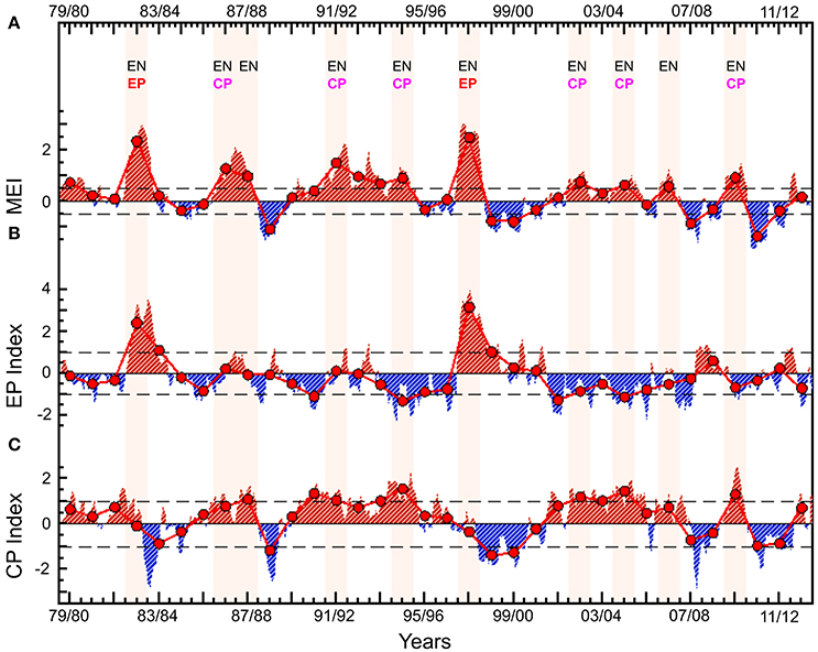
Figure 1. Climate indices of El Niño events during the period 1979–2014. Monthly anomalies of (A) Multivariate ENSO Index; (B) Eastern Pacific El Niño Index; and (C) Central Pacific El Niño Index. Annual mean anomalies (thick red line and large dots) were calculated by averaging the monthly anomalies over the periods from June (of year t) to May (of year t + 1). Classification of El Niño as EP and CP is based on Radenac et al. (2012) and Yu et al. (2012). EN, El Niño, EP, Eastern Pacific, CP, Central Pacific.

Results and Discussion

EP and CP El Niño Impact on Oceanic Phytoplankton

The confidence level of the response patterns (Figures 2A,B) identified with the statistical analysis is assessed as very likely (i.e., within 90–100% probability range; IPCC Climate Change, 2013). During EP El Niño, at the global scale, the median chlorophyll impact is found to be −6.5%, mostly driven by a large decrease of −7.5% in the tropics (3,529 pixels), and limited increases in the Northern and Southern Hemispheres of +6.6 and +5.5% respectively (505 and 643 pixels respectively). During CP El Niño, global median chlorophyll impact is found to be −7.4%, which is the resultant of large decrease estimated for the tropics of −8.7% (1,948 pixels), and limited decrease estimated for the Northern Hemisphere of −4.9% (342 pixels) and increase for the Southern Hemisphere of +4.1% (500 pixels) (Supplementary Table 1 and Supplementary Figure 2). The impact values are estimated based on EP and CP indices equal to one (annual mean index values over the period 1997–2012 are presented in Figure 1). It is noteworthy that monthly impact values may be ~3–4 times higher, particularly during the peak of El Niño events, such as in December 1997 when the EP El Niño index reached value of 3.9, and in December 2009 when the CP El Niño index reached value of 2.6 (Yu, 2016).

FIGURE 2

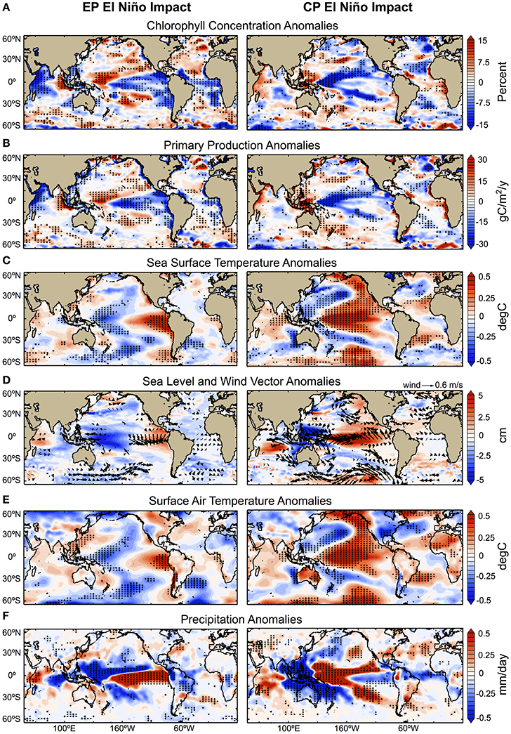
Figure 2. Observed impacts of Eastern and Central Pacific El Niño on biological and physical variables during 1997–2012. Annual mean anomalies are regressed onto the (left) EP and (right) CP El Niño indices. Increase and decrease are indicated by positive (red) and negative (blue) anomalies respectively. (A) Chlorophyll Concentration anomalies; (B) Primary Production anomalies; (C) SST anomalies; (D) SL and wind anomalies; (E) Surface Air Temperature anomalies; and (F) Precipitation anomalies. In all panels, stippling indicates where the linear regression coefficients are significant at the 90% confidence level over the entire period of 1997–2012. The statistical significance of these regression coefficients was estimated according to Student t-test and considering the autocorrelation of the time-series. The impact values are estimated based on EP and CP indices equal to one.

The regions identified as most sensitive to the EP and CP El Niño climatic perturbations compare well with the locations where significant trends in chlorophyll have been estimated previously using contemporary satellite records (Vantrepotte and Mélin, 2011; Gregg and Rousseaux, 2014; Hoegh-Guldberg et al., 2014). Furthermore, the biological and physical response patterns to each type of El Niño observed in the present work over the satellite record of 1997–2012 are consistent with contemporary case studies of specific EP and CP El Niño events in the Equatorial Pacific (Turk et al., 2011; Gierach et al., 2012; Radenac et al., 2012), the Indian Ocean (Webster et al., 1999), the continental U.S. (Yu et al., 2012; Yu and Zou, 2013), and the global oceans (Behrenfeld et al., 2001; Messié and Chavez, 2012, 2013). In addition, the response patterns observed for the physical variables have also been shown to persist over decadal timescales during the period 1979–2014 (see Section Physical Forcing Mechanisms Associated with El Niño Variability). Finally, when both EP and CP indices are equal to one, the sum of the observed impacts observed in response to EP and CP El Niño (Supplementary Figure 3) is shown to be approximately equal to the impact observed using the MEI. This is coherent as the MEI encompasses effects of both EP and CP El Niño variations.

Major Factors Influencing Phytoplankton Growth

To understand the specific influence of the climatic perturbations on phytoplankton, we must first identify the mechanisms driving the biophysical interactions at the global and regional scales. Phytoplankton growth is light-limited at high-latitudes where annual mean nitrate concentration is high and monthly means of chlorophyll and PAR show positive correlation, and monthly means of chlorophyll and MLD show negative correlation (i.e., chlorophyll increases when MLD is shallower and light availability is higher; Figures 3A,B). In contrast, phytoplankton growth is nutrient-limited in the tropics and subtropics where light-availability is plentiful all-year-round, annual mean nitrate concentration is low (Figure 3C) and monthly means of chlorophyll and MLD show positive correlation (i.e., chlorophyll increases when MLD is deeper, and nutrient-rich deep waters are mixed with nutrient-poor surface waters, increasing nutrient availability for phytoplankton growth to occur). Further to nutrient supply from vertical mixing, the tropics display strong zonal surface currents (Figure 3D), which can increase horizontal advection of nutrient and, in turn, enhance phytoplankton growth. The latter mechanism can explain the weak correlation coefficients observed between monthly means of chlorophyll and MLD in some areas of the tropics and subtropics. Finally, the negative correlation shown between monthly means of chlorophyll and MLD in the eastern Equatorial Pacific is coherent with the observed high annual mean nitrate concentration (i.e., macronutrients are not limiting; Figure 3C), and previously reported iron limitation (i.e., limiting trace nutrient) occurring in the region (Gordon et al., 1997; Moore et al., 2013). In some specific areas of the North and Equatorial Pacific Ocean, and the Southern Ocean, known as High Nutrient-Low Chlorophyll (HNLC) regions, the low trace nutrients concentration (iron, manganese) present all year round, limit phytoplankton production.

FIGURE 3

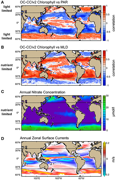
Figure 3. Major factors influencing phytoplankton growth. (A) Correlation map between monthly surface chlorophyll concentration from OC-CCIv2 and photosynthetically active radiation (PAR) over the period Sep. 1997 to Dec. 2012; (B) Correlation map between monthly surface chlorophyll concentration from OC-CCIv2 and mixed layer depth (MLD) estimated using SODA vertical profiles of temperature over the period Sep. 1997 to Dec. 2008; (C) Annual average surface concentration of nitrate (μmol/l) from World Ocean Atlas Climatology; and (D) Annual average zonal surface currents (m/s) from OSCAR NOAA. (A,B) Positive correlation is indicated in red color and negative correlation in blue color. Contour lines indicate correlation coefficients that are significant at the 90% confidence level based on Pearson correlation coefficients. (D) Positive values indicate eastward currents and negative values westward currents.

The results presented in Figure 3 are consistent with the different physical regimes and global climatological relationships previously demonstrated between open ocean satellite surface observations of chlorophyll and subsurface parameters of MLD, thermocline and nutricline depths at global scale (Wilson and Coles, 2005; Messié and Chavez, 2012; Brewin et al., 2014) and in the Equatorial Pacific (Turk et al., 2011; Gierach et al., 2012; Radenac et al., 2012; Lee et al., 2014). In coastal regions, phytoplankton production can be modified further by local supply of nutrients through coastal upwelling, riverine input (e.g., Turner et al., 2003) or atmospheric dust deposition (Abram et al., 2003; Jickells et al., 2005). In Polar regions, changes in phytoplankton production are tightly coupled to variations in sea-ice extent and timing of retreat, which can affect light and nutrient availability (Kahru et al., 2011, 2016; Arrigo and van Dijken, 2015).

Physical Forcing Mechanisms Associated with El Niño Variability

The results of the biological and physical responses to the EP and CP types of El Niño, which are statistically significant, are presented in Figures 2, 4, and with an estimate of uncertainty in the observational product in Figure 5. In the Equatorial Pacific Ocean, where ENSO activity is rooted, an EP El Niño event is generated when easterly trade winds weaken in the east and westerlies prevail in the west (Figures 2D, 4C), pushing warmer, nutrient-poor waters to the east (along the coast of Peru and Chile), reducing nutrient availability, leading to a decrease in chlorophyll and PP in the eastern Pacific of −12 ± 5% and −56 ± 21 TgC/y (Figures 2A,B, 5). In contrast, a CP El Niño event is generated when easterly trade winds in the east and westerlies in the west are enhanced (Figures 2D,4C), pushing warmer, nutrient-poor waters to the central Equatorial Pacific, reducing nutrient availability, which is associated with a decrease in chlorophyll and PP of −14 ± 5% and −68 ± 22 TgC/y (Figures 2A,B, 5). In both cases, regional decreases in phytoplankton are caused by variations in horizontal and vertical advective fluxes responsible for the transport of nutrients to the surface layer, which are driven by perturbation in the wind forcing (Ashok and Yamagata, 2009; Gierach et al., 2012; Messié and Chavez, 2012, 2013; Radenac et al., 2012). Enhanced advection is also observed during CP El Niño in the tropical Atlantic Ocean as the Equatorial easterlies intensify in the east (Figures 2D, 4C), bringing warmer, nutrient-poor waters to around 15°N (Richter et al., 2012), and leading to decreases in chlorophyll and PP of −8 ± 3% and −10 ± 5 TgC/y (Figures 2A,B, 5). In the Indian Ocean, Equatorial easterlies are found to intensify during EP El Niño, promoting horizontal advection of warmer and nutrient-poor waters to the western-side of the basin (Figure 2C) (Webster et al., 1999), resulting in decreases in chlorophyll and PP of −11 ± 4% and −82 ± 31 TgC/y (Figures 2A,B, 5), whereas in the eastern-side, the observed increases in chlorophyll and PP of +7 ± 3% and +13 ± 5 TgC/y (Figures 2A,B, 5) are likely to be driven by enhanced upwelling (Figure 2C) and atmospheric fallout from Indonesian fires and, further north in the basin, by enhanced nutrient supply from the Ganges and Brahmaputra rivers. The latter processes are consistent with the strong increase in fires (Wooster et al., 2012; Huijnen et al., 2016) and dust deposition reported off the west coast of Sumatra (Murtugudde et al., 1999; Abram et al., 2003), and the increased precipitation patterns observed over the Himalayas (Figure 4F). Furthermore, in some regions, these processes may not be sufficient to explain the observed variations in chlorophyll and PP, and other processes may be involved, such as atmospheric dust deposition from desert (e.g., EP El Niño impact in the Cape Verde Sea), extent and duration of sea-ice cover in the Artic (e.g., EP El Niño impact in the Bering and Labrador Seas), and iron limitation in HNLC regions (e.g., EP and CP El Niño impact in the Pacific sector of the Southern Ocean). Further information would be required to validate these forcing mechanisms.

FIGURE 4

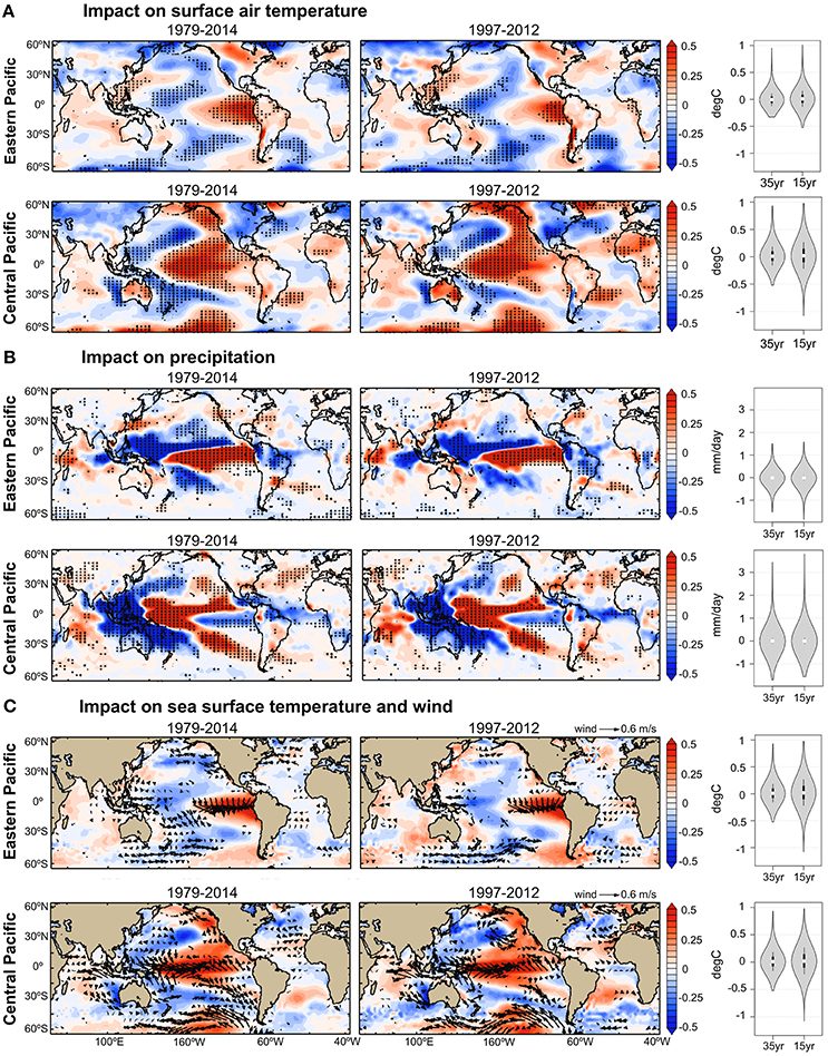
Figure 4. Observed impacts of Eastern and Central Pacific El Niño on physical variables during the periods 1979–2014 and 1997–2012. Annual mean anomalies are regressed onto the annual mean EP and CP El Niño indices. Increase and decrease are indicated by positive (red) and negative (blue) anomalies respectively. In all panels, stippling indicates where the regression coefficients are significant at the 90% confidence level over the entire 35-year period (1979–2014; left panels) and 15-year period (1997–2012; central panels). The statistical significance of these regression coefficients was estimated according to Student t-test and considering the autocorrelation of the time-series. The probability density distributions of the regression coefficients are shown in gray shading for the 35 and 15-year periods (right panels). The white dot indicates the position of the median, and the upper and lower ends of the black rectangle indicate the upper and lower quartiles respectively. Surface air temperature and precipitation datasets are from NCEP/NCAR reanalysis, and sea surface temperature and wind datasets are from ECMWF reanalysis (see Table 1). The impact values are estimated based on EP and CP indices equal to one.

FIGURE 5

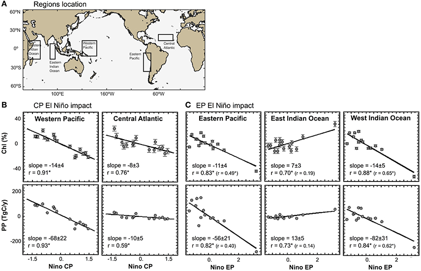
Figure 5. Regional impacts of ENSO climatic perturbations during the period 1997–2012. (A) Location of the areas used in the estimation of regional EP and CP El Niño impact during the period 1997–2012; (B) Annual mean relative anomalies of Chlorophyll (in %) vs. EP index, and annual mean anomalies of Primary Production (in TgC/y) versus EP index; and (C) Annual mean relative anomalies of Chlorophyll (in %) versus CP index, and annual mean anomalies of Primary Production (in TgC/y) vs. CP index. The slope is provided ±Standard Error. Significant Pearson correlation coefficients at the 90% confidence level are indicated with a star. (B) The Pearson correlation coefficients shown in parenthesis are based on the analyses run without including 1997–1998 El Niño event. (B,C) Error bars for each point indicate the standard error based on the total number of observations in each corresponding box region. The standard error is calculated based on the root-mean-square-difference and bias observations provided in OC-CCIv2.

The estimation of EP impact relies heavily on the El Niño event of 1997–1998, which was the single, important EP event that occurred within the relatively short time span of 15 years for which we have the OC-CCI data. To evaluate the impact that this single event had on our results, the correlation analyses have been rerun without the 1997–1998 event. In this case, the influence of EP El Niño on phytoplankton chlorophyll concentration remained significant in the Eastern Pacific Ocean and Western Indian Ocean, but not in the Eastern Indian Ocean region (Figure 5), indicating further that other regional climate oscillations are important drivers at basin scale (please see discussion in Section Implications for Climate Impact Research). In addition, the analyses of the EP and CP impact on physical processes are further validated on interannual to decadal timescales in Figure 4. The regression coefficients of the EP and CP impact estimated for the two periods 1979–2014 and 1997–2012 show similar spatial patterns and frequency distributions for the physical variables studied. This indicates that the results presented in Figure 2 (period 1997–2012) are not skewed to the 1997–1998 EP El Niño event, and that the impact patterns are stable over multi-decadal time scales (35-year), at least for the physical variables. Since phytoplankton dynamics are at the mercy of these physical conditions, we postulate that the inference may also hold for the biological variables studied here (e.g., Figures 2, 5).

Implications for Climate Impact Research

Phytoplankton have a high turn-over rate, responding to changes in their environment at scales ranging from seconds to days, and illustrating well the first-level biological response to environmental changes. At the same time, because of decadal-scale variabilities in the physical forcing fields, it is generally understood that multi-decadal, uninterrupted data are needed to evaluate the impact of climate change on marine ecosystems. Such data are only rarely available from limited in situ time series stations (mostly coastal). Furthermore, satellite ocean-color sensors have provided barely two decades of uninterrupted data that can be used for climate research (Sathyendranath and Krasemann, 2014). In this context, El Niño variability, together with other large-scale inter-annual variations, provides an important vehicle to study how phytoplankton in the ocean (and hence the organisms at higher trophic levels) respond to climate variability and identify the driving processes. In turn, monitoring and analysis of long-term changes in these driving processes would help us to improve understanding of projected impact of long-term climate changes on the marine ecosystem.

In the present study, we have addressed potential issues related to the collection of continuous ocean-color time-series and processing of climate-quality products, to the study of biophysical interactions, El Niño remote-forcing mechanisms and their propagation, and the diversity of El Niño events by: (i) using the longest, error-characterized, biased-corrected, climate-quality controlled, global scale merged satellite ocean-color data product from ESA Ocean-Color Climate Change Initiative project; (ii) analyzing in synergy satellite ocean-color data record and reanalysis datasets to identify the dominant mechanisms driving the biophysical interactions; (iii) characterizing local and remote influences of El Niño types on key driving variables of SST, Sea Level, wind, and precipitation; (iv) analyzing annual mean signal centered around the peak timing of El Niño activity in boreal winter; and (v) selecting EP and CP indices, which are computed to enhance differences in SST anomalies from the two most eastern and central Pacific Niño1+2 and Niño 4 regions respectively.

Our work highlights the importance of maintaining a long time series of consistent ocean-color products, to be able to evaluate the impact of climate variability on the biological fields. For example, our results on the impact of EP events could be improved when additional EP events can be incorporated into the analyses, such that the results would no longer be so heavily dependent on a single EP event, as was the case here. More data from longer time series are also essential to explore non-linearities in biological responses, which could not be investigated here because of limited data availability.

Our analysis shows that the modification of global oceanic phytoplankton under climate change cannot be forecast with respect to changes in a single ocean property. Rather, a range of environmental properties may be involved (e.g., advection in three dimensions, wind, riverine input, atmospheric dust deposition, stratification) whose intensity may vary on a regional basis. The statistical approach to study El Niño impact applied here has permitted us to characterize a complex mosaic of biological responses illustrating that different forcing dominates in different regions. The biophysical processes driving phytoplankton production are summarized in Figure 6 in the form of an atlas of EP and CP El Niño impact. The influence of CP and EP El Niño events can be felt in the global oceans, although the affected regions are predominantly located in the tropics and subtropics encompassing 66–67% of the total areas affected, and the remaining 33–34% are areas located in high-latitudes. In the tropics and subtropics, 35–39% of the total affected areas showed a decrease in PP associated with reduced nutrient availability during CP and EP El Niño respectively, whereas in higher latitudes 19–20% of the affected areas showed an increase in PP associated with reduced light limitation (Figure 3). Even though, the percent of total affected areas are relatively similar between CP and EP El niño events, the regional differentiation is marked, and may be of opposing sign (e.g., along the coast of Peru and Chile, the Benguela upwelling, the Great Barrier Reef), or affected during an EP event but not during a CP event (e.g., in the tropical eastern and western Pacific). Several process-orientated studies have further highlighted the important role played by horizontal processes (together with vertical processes) in the supply of nutrients in the surface layer, and specifically demonstrated significant impacts in Winter new primary production in the North Pacific transition zone (Ayers and Lozier, 2010), inter-annual variations of chlorophyll concentration in the Equatorial Pacific (Gierach et al., 2012; Messié and Chavez, 2013; Dave and Lozier, 2015) and the Red Sea (Raitsos et al., 2015), and decadal variations in phytoplankton abundance in the North Atlantic Subpolar Gyre (Martinez et al., 2015). Thus, both the development of statistical methods to study climate impact, and the assessment of the future evolution of regional physical forcing processes may help us to understand phytoplankton responses to climate change and improve confidence in our projection of future ecosystem state (Bopp et al., 2013; Boyd et al., 2014). The first assessment based on a biogeochemical and ecosystem model output of chlorophyll response to the EP and CP types of El Niño was shown to compare well with remotely-sensed observations in the Equatorial Pacific (Lee et al., 2014). However, the response to El Niño variability projected from biogeochemical and ecosystem models is yet to be investigated at the global scale.

FIGURE 6

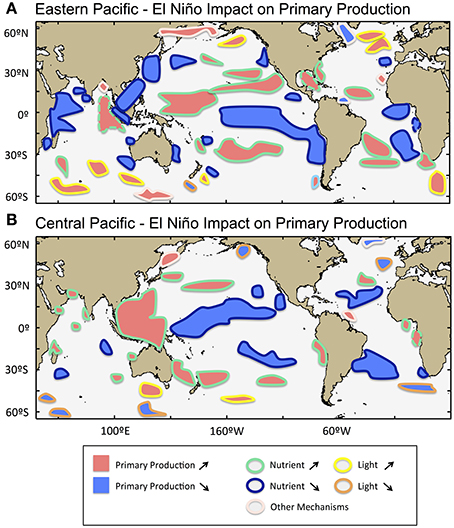
Figure 6. Schematic atlas of the influence of El Niño variability on oceanic phytoplankton in the global oceans. (A) Eastern Pacific El Niño influence, and (B) Central Pacific El Niño influence. Increase and decrease in primary production (PP) are indicated in red and blue filled colors respectively. The color contours provide information about the controlling biophysical mechanisms (which are described in Section Physical Forcing Mechanisms Associated with El Niño Variability and Mapped in Figure 3): (yellow) PP is nutrient-limited; (dark blue) PP is enhanced by nutrient availability; (orange) PP is light-limited; (turquoise) PP is enhanced by light availability; (light pink or dashed contour) PP may be further controlled by other mechanisms, such as sea-ice melting, atmospheric dust deposition and availability of trace nutrients. The contour delineation of the influence of EP and CP El Niño is generated based on information displayed in Figure 2 and Supplementary Figure 4.

Notwithstanding the dominant influence of El Niño on global climate patterns, other driving factors may enhance or weaken the observed biophysical impact. Examining links between El Niño and inter-annual and decadal climate oscillations (Di Lorenzo et al., 2010; Izumo et al., 2010) may provide further insights toward improving projection of environmental properties and associated phytoplankton responses to climate forcing at global and regional scales. The regional variations associated with El Niño may be superimposed on long-term warming trends (Bopp et al., 2013; IPCC Climate Change, 2013; Boyd et al., 2014; Kumar et al., 2016) and regional-scale oscillations at sub-seasonal and seasonal scales associated with other large-scale climate modes of variability, such as the Atlantic Multidecadal Oscillation (AMO) and Pacific Decadal Oscillation (PDO; Martinez et al., 2009), the North Pacific Gyre Oscillation (NPGO; Di Lorenzo et al., 2008, 2010; Messié and Chavez, 2013), the monsoon and Indian Ocean Dipole (IOD; Saji et al., 1999; Ashok et al., 2007; Izumo et al., 2010; Brewin et al., 2012; Currie et al., 2013). As a result, the regional climate response is not a simple function of the strength and centroid location of an El Niño event. Further, the regional patterns observed using EP and CP El Niño indices may be sufficient to explain only a fraction of all the regional variations on a year-to-year basis (except perhaps where El Niño is likely to dominate the variability of the system such as in the Equatorial Pacific region). For instance, in the Indian Ocean, the ENSO and IOD indices can account for ~30% and 12% respectively of the regional variations in SST (Saji et al., 1999), and years of co-occurrence of positive IOD and El Niño events may provide positive feedbacks to the SST (Kumar et al., 2016). Therefore, some apparent differences will show between the observed impact of El Niño on biological and physical variables, and the corresponding anomalies.

Implications for the Oceanic Ecosystem and Carbon Cycle

Phytoplankton are at the base of the food chain and transfer energy to higher trophic levels. This transfer of energy has a knock-on effect on fisheries and dependent human societies especially in highly productive and coastal upwelling regions, as well as coral reef ecosystems. The larvae of many marine species graze on phytoplankton during this most vulnerable stage of their lives. Hence, changes in phytoplankton population associated with climate variability may propagate rapidly up the marine food chain and profoundly alter the functioning of marine ecosystems (Platt et al., 2003; Edwards and Richardson, 2004; Lo-Yat et al., 2011). In addition, changes in environmental conditions associated with EP and CP El Niño events have been shown to impact mesozooplankton community with variable time lags in the northern California Current, which in turn can affect top down control on phytoplankton, and disrupt the pelagic food chain (Fisher et al., 2015). Following EP and CP El Niño events, quite different impact on commercially important fisheries have been reported in anchovy catches in the Humboldt Current Large Marine Ecosystem (Jackson et al., 2011) and tuna catches in the Indian Ocean (Kumar et al., 2014). In coral reef ecosystems, changes in phytoplankton population and mass bleaching following an El Niño event can critically affect fisheries, recreation, and tourism services (Hoegh-Guldberg, 1999; Abram et al., 2003; Lo-Yat et al., 2011). Recent analysis in the Andaman Sea, southeast Bay of Bengal, has further demonstrated that differences both in intensity and timing of SST warming associated with EP and CP El Niño events, can determine the extent of mass coral bleaching (Lix et al., 2016). In this context, regional differentiation of the impact of each type of El Niño events (Figure 6) may provide important information to delineate and establish protected coral reef and fishing areas to facilitate their recovery.

The oceanic carbon sink is part of a very active, natural cycle, in which phytoplankton in the surface layer of the ocean fix, by photosynthesis, dissolved CO₂ in the water into organic matter, some of which subsequently sinks below the mixed layer. Through the associated decrease in the partial pressure of CO₂ in the surface ocean, phytoplankton contribute to the drawdown of dissolved CO₂ from the ocean surface layer (Hauck et al., 2015), which in turn help to modulate the increase in anthropogenic atmospheric CO₂. The estimated El-Niño-driven changes in PP at the regional scale can be considerable, reaching values of −57 ± 21 and−68 ± 22 TgC/y in the Eastern and Central Equatorial Pacific Ocean during EP and CP types of El Niño respectively (Figure 5). However, to provide a more complete picture on the influence on the carbon cycle, further investigations are required to quantify the impact of El Niño on carbon export and associated changes in air-sea CO₂ fluxes. The buffering action of the ocean in the carbon cycle is non-linear—it varies with the water temperature (solubility pump), alkalinity (carbonate pump), biological productivity and demineralization (biological pump); the impact on environmental and ecosystem properties must be evaluated at the appropriate scale to allow investigation of the underlying mechanisms driving the variability in the ocean carbon cycle.

As the frequency of extreme El Niño events and the relative frequency of occurrence of CP-El Niño/EP-El Niño are projected to increase under climate warming (Yeh et al., 2009; Lee and McPhaden, 2010; Cai et al., 2015), it is essential to refine our regional assessment of climate impact associated with El Niño variability. The atlas of impact of CP and EP types of El Niño on oceanic phytoplankton (Figure 6) can be used for societal benefit. It provides key climate impact information that can allow us to better inform fisheries management on possible risks and opportunities associated with El Niño events, and support more effectively mitigation and adaptation plans for local fisheries-dependent societies. The atlas information can also provide observational basis to test model predictions of the impact of climate change on the marine ecosystem. Finally, from a biogeochemical perspective, such insights on El Niño variability impact are needed to improve our understanding of the buffering capacity of the oceanic carbon cycle under climate change.

Author Contributions

MFR designed and implemented the research. MFR, SS, RB, TJ provided materials and analysis tools. MFR, SS, RB, TJ, DR, and TP discussed the results and contributed to the writing of the manuscript.

Funding

MFR is funded through a European Space Agency Living Planet Fellowship Grant Ref Number (CCI-LPF-EOPS-MM-16-0078). SS, TJ, and TP are funded through ESA Ocean Color Climate Change Initiative program. SS, MFR, RB, and DR are funded through the NERC's UK National Centre for Earth Observation.

Conflict of Interest Statement

The authors declare that the research was conducted in the absence of any commercial or financial relationships that could be construed as a potential conflict of interest.

Acknowledgments

This work is a contribution to the European Space Agency Ocean Color Climate Change Initiative (ESA OC-CCI), the European Space Agency Living Planet Fellowship program (CLIMARECOS), and to the NERC National Centre for Earth Observation (NCEO). The authors thank the ESA CCI teams for providing OC-CCI chlorophyll data, SL-CCI sea level data, and NCEO-ESA-SST-CCI sea surface temperature data. The authors further acknowledge TWAP for providing primary production data; NASA for providing SeaWiFS and MODIS PAR data; NOAA for providing NCEP/NCAR air surface temperature and precipitation reanalysis data; ECMWF for providing ERA Interim wind and sea surface temperature reanalysis data; and SODA for providing ocean temperature reanalysis data. The authors thank James Dingle for technical support with the OC-CCI data processing, Stéphane Saux-Picart for help in processing the mixed layer depth, Sang-Wook Yeh for discussion about El Niño phenomenon, and Eleni Papathanasopoulou for discussion about socio-economic impacts. The authors wish to acknowledge use of the Ferret program for analysis and graphics in this paper—Ferret is a product of NOAA's Pacific Marine Environmental Laboratory (information is available at http://ferret.pmel.noaa.gov/Ferret/). The authors would also like to acknowledge the Nature Method on-line web-tool BoxPlotR (http://boxplot.tyerslab.com/), which was used to generate the boxplots, and Dimitrios Kleftogiannis for information about boxplot analysis tools. We acknowledge the two reviewers for providing constructive comments on our manuscript.

Supplementary Material

The Supplementary Material for this article can be found online at: https://www.frontiersin.org/article/10.3389/fmars.2017.00133/full#supplementary-material

References

Ablain, M., Cazenave, A., Larnicol, G., Balmaseda, M., Cipollini, P., Faugère, Y., et al. (2015). Improved sea level record over the satellite altimetry era (1993–2010) from the Climate Change Initiative project. Ocean Sci. 11, 67–82. doi: 10.5194/os-11-67-2015

CrossRef Full Text | Google Scholar

Abram, N. J., Gagan, M. K., McCulloch, M. T., Chappell, J., and Hantoro, W. S. (2003). Coral reef death during the 1997 Indian Ocean Dipole linked to Indonesian wildfires. Science 301, 952–955. doi: 10.1126/science.1083841

PubMed Abstract | CrossRef Full Text | Google Scholar

Antoine, D., André, J.-M., and Morel, A. (1996). Oceanic primary production: 2. Estimation at global scale from satellite (Coastal Zone Color Scanner) chlorophyll. Glob. Biogeochem. Cycles 10, 57–69. doi: 10.1029/95GB02832

CrossRef Full Text | Google Scholar

Arrigo, K. R., and van Dijken, G. L. (2015). Continued increases in Arctic Ocean primary production. Prog. Oceanogr. 136, 60–70. doi: 10.1016/j.pocean.2015.05.002

CrossRef Full Text | Google Scholar

Ashok, K., Behera, S. K., Rao, S. A., Weng, H., and Yamagata, T. (2007). El Niño Modoki and its possible teleconnection. J. Geophys. Res. 112:C11007. doi: 10.1029/2006JC003798

CrossRef Full Text | Google Scholar

Ashok, K., and Yamagata, T. (2009). The El Niño with a difference. Nature 461, 481–484. doi: 10.1038/461481a

PubMed Abstract | CrossRef Full Text | Google Scholar

Ayers, J. M., and Lozier, M. S. (2010). Physical controls on the seasonal migration of the North Pacific transition zone chlorophyll front. J. Geophys. Res. 115:C05001. doi: 10.1029/2009JC005596

CrossRef Full Text | Google Scholar

Behrenfeld, M. J., Boss, E., Siegel, D. A., and Shea, D. M. (2005). Carbon-based ocean productivity and phytoplankton physiology from space. Glob. Biogeochem. Cycles 19:GB1006:1-14. doi: 10.1029/2004gb002299

CrossRef Full Text | Google Scholar

Behrenfeld, M. J., O'Malley, R. T., Siegel, D. A., McClain, C. R., Sarmiento, J. L., Feldman, G. C., et al. (2006). Climate-driven trends in contemporary ocean productivity. Nature 444, 752–755. doi: 10.1038/nature05317

PubMed Abstract | CrossRef Full Text | Google Scholar

Behrenfeld, M. J., Randerson, J. T., McClain, C. R., Feldman, G. C., Los, S. O., Tucker, C. J., et al. (2001). Biospheric primary production during an ENSO transition. Science 291, 2594–2595. doi: 10.1126/science.1055071

PubMed Abstract | CrossRef Full Text | Google Scholar

Bopp, L., Resplandy, L., Orr, J. C., Doney, S. C., Dunne, J. P., Gehlen, M., et al. (2013). Multiple stressors of ocean ecosystems in the 21st century: projections with CMIP5 models. Biogeosciences 10, 6225–6245. doi: 10.5194/bg-10-6225-2013

CrossRef Full Text | Google Scholar

Boyd, P. W., Lennartz, S. T., Glover, D. M., and Doney, S. C. (2014). Biological ramifications of climate-change-mediated oceanic multi-stressors. Nat. Clim. Change 5, 71–79. doi: 10.1038/nclimate2441

CrossRef Full Text | Google Scholar

Boyer, T. P., Antonov, J. I., Baranova, O. K., Coleman, C., Garcia, A., Grodsky, D. R., et al. (2013). NOAA Atlas NESDIS 72. World Ocean Database 2013. Silver Spring, MD.

Google Scholar

Brewin, R. J. W., Hirata, T., Hardman-Mountford, N. J., Lavender, S. J., Sathyendranatha, S., and Barlow, R. (2012). The influence of the Indian Ocean Dipole on interannual variations in phytoplankton size structure as revealed by Earth Observation. Deep Sea Res. II 77–80, 117–127. doi: 10.1016/j.dsr2.2012.04.009

CrossRef Full Text | Google Scholar

Brewin, R. J. W., Mélin, F., Sathyendranath, S., Steinmetz, F., Chuprin, A., and Grant, M. (2014). On the temporal consistency of chlorophyll products derived from three ocean-colour sensors. ISPRS J. Photogramm. Remote Sens. 97, 171–184. doi: 10.1016/j.isprsjprs.2014.08.013

CrossRef Full Text | Google Scholar

Cai, W., Santoso, A., Wang, G., Yeh, S.-Y., An, S.-I., et al. (2015). ENSO and greenhouse warming. Nature 5, 849–859. doi: 10.1038/nclimate2743

CrossRef Full Text | Google Scholar

Capotondi, A., Wittenberg, A. T., Newman, M., Di Lorenzo, E., Yu, J.-Y., et al. (2015). Understanding ENSO diversity. Bull. Am. Meteorol. Soc. 96, 921–938. doi: 10.1175/BAMS-D-13-00117.1

CrossRef Full Text | Google Scholar

Carton, J. A., and Giese, B. S. (2008). A reanalysis of ocean climate using Simple Ocean Data Assimilation (SODA). Monthly Weather Rev. 136, 2999–3017. doi: 10.1175/2007MWR1978.1

CrossRef Full Text | Google Scholar

Chavez, F. P., Messié, M., and Pennington, J. T. (2011). Marine primary production in relation to climate variability and change. Ann. Rev. Mar. Sci. 3, 227–260. doi: 10.1146/annurev.marine.010908.163917

PubMed Abstract | CrossRef Full Text | Google Scholar

Couto, A. B., Holbrook, N. J., and Maharaj, A. M. (2013). Unravelling eastern pacific and central pacific ENSO contributions in south pacific chlorophyll-a variability through remote sensing. Remote Sens. 5, 4067–4087. doi: 10.3390/rs5084067

CrossRef Full Text | Google Scholar

Currie, J. C., Lengaigne, M., Vialard, J., Kaplan, D. M., Aumont, O., Naqvi, S. W. A., et al. (2013). Indian Ocean dipole and El Niño/southern oscillation impacts on regional chlorophyll anomalies in the Indian Ocean. Biogeosciences 10, 6677–6698.

Google Scholar

Dave, A. C., and Lozier, M. S. (2015). The impact of advection on stratification and chlorophyll variability in the equatorial Pacific. Geophys. Res. Lett. 42, 4523–4531. doi: 10.1002/2015GL063290

CrossRef Full Text | Google Scholar

de Boyer Montégut, C., Madec, G., Fischer, A. S., Lazar, A., and Ludicone, D. (2004). Mixed layer depth over the global ocean: an examination of profile data and a profile-based climatology. J. Geophys. Res. 109:C12003. doi: 10.1029/2004jc002378

CrossRef Full Text | Google Scholar

Dee, D. P., Uppala, S. M., Simmons, A. J., Berrisford, P., Poli, P., et al. (2011). The ERA-Interim reanalysis: configuration and performance of the data assimilation system. Q. J. R. Meteorol. Soc. 137, 553–597. doi: 10.1002/qj.828

CrossRef Full Text | Google Scholar

Di Lorenzo, E., Cobb, K. M., Furtado, J. C., Schneider, N., Anderson, B. T., et al. (2010). Central Pacific El Niño and decadal climate change in the North Pacific Ocean. Nat. Geosci. 3, 762–765. doi: 10.1038/ngeo984

CrossRef Full Text | Google Scholar

Di Lorenzo, E., Schneider, N., Cobb, K. M., Franks, P. J. S., Chhak, K., et al. (2008). North Pacific Gyre Oscillation links ocean climate and ecosystem change. Geophys. Res. Lett. 35:L08607. doi: 10.1029/2007GL032838

CrossRef Full Text | Google Scholar

Edwards, M., and Richardson, A. J. (2004). Impact of climate change on marine pelagic phenology and trophic mismatch. Nature 430, 881–884. doi: 10.1038/nature02808

PubMed Abstract | CrossRef Full Text | Google Scholar

Fisher, J. L., Peterson, W. T., and Rykaczewski, R. R. (2015). The impact of El Niño events on the pelagic food chain in the northern California Current. Glob. Change Biol. 21, 4401–4414. doi: 10.1111/gcb.13054

PubMed Abstract | CrossRef Full Text | Google Scholar

Frouin, R., McPherson, J., Ueyoshi, K., and Franz, B. A. (2012). A time series of photosynthetically available radiation at the ocean surface from SeaWiFS and MODIS data. Remote Sens. Mar. Environ. II Proc. SPIE 8525, 852519. doi: 10.1117/12.981264

CrossRef Full Text | Google Scholar

Gierach, M. M., Lee, T., Turk, D., and McPhaden, M. J. (2012). Biological response to the 1997-98 and 2009-10 El Niño events in the equatorial Pacific Ocean. Geophys. Res. Lett. 39:L10602. doi: 10.1029/2012GL051103

CrossRef Full Text | Google Scholar

Gordon, R. M., Coale, K. H., and Johnson, K. S. (1997). Iron distributions in the equatorial Pacific: Implications for new production. Limnol. Oceanogr. 42, 419–431. doi: 10.4319/lo.1997.42.3.0419

CrossRef Full Text | Google Scholar

Gregg, W., and Rousseaux, C. S. (2014). Decadal trends in global pelagic ocean chlorophyll: a new assessment integrating multiple satellites, in situ data, and models. J. Geophys. Res. Oceans 119, 5921–5933. doi: 10.1002/2014JC010158

PubMed Abstract | CrossRef Full Text | Google Scholar

Hauck, L., Völker, C., Wolf-Gladrow, D. A., Laufkötter, C., Vogt, M., et al. (2015). On the Southern Ocean CO2 uptake and the role of the biological carbon pump in the 21st century. Glob. Biogeochem. Cycles 29, 1451–1470. doi: 10.1002/2015GB005140

CrossRef Full Text | Google Scholar

Hoegh-Guldberg, O. (1999). Climate change, coral bleaching and the future of the world's coral reefs. Mar. Freshwater Res. 50, 839–866. doi: 10.1071/MF99078

CrossRef Full Text | Google Scholar

Hoegh-Guldberg, O., Cai, R., Brewer, P. G., Fabry, V. J., Hilmi, K., et al. (2014). “IPCC Climate Change 2014: Impacts, Adaptation, and Vulnerability Chapter 30 – The Ocean,” in Contribution of Working Group II to the Fifth Assessment Report of the Intergovernmental Panel on Climate Change (Cambridge, UK; New York, NY: Cambridge University Press).

Google Scholar

Huijnen, V., Wooster, M. J., Kaiser, J. W., Gaveau, D. L. A., Flemming, J., Parrington, M., et al. (2016). Fire carbon emissions over maritime southeast Asia in 2015 largest since 1997. Sci. Rep. 6:26886. doi: 10.1038/srep26886

PubMed Abstract | CrossRef Full Text | Google Scholar

IPCC Climate Change (2013). “The Physical Science Basis Summary for Policymakers,” in Contribution of Working Group I to the Fifth Assessment Report of the Intergovernmental Panel on Climate Change, eds T. F. Stocker, D. Quin, G. -K. Plattner, M. Tignor, S. K. Allen, et al. (Cambridge, UK; New York, NY: Cambridge University Press).

Izumo, T., Vialard, J., Lengaigne, M., De Boyer Montegut, C., Behera, S. K., Luo, J. J., et al. (2010). Influence of the state of the Indian Ocean Dipole on the following year's El Niño. Nat. Geosci. 3, 168–172. doi: 10.1038/ngeo760

CrossRef Full Text | Google Scholar

Jackson, T., Bouman, H. A., Sathyendranath, S., and Devred, E. (2011). Regional-scale changes in diatom distribution in the Humboldt upwelling system as revealed by remote sensing: implications for fisheries. ICES J. Mar. Sci. 68, 729–736. doi: 10.1093/icesjms/fsq181

CrossRef Full Text | Google Scholar

Jickells, T. D., An, Z. S., Andersen, K. K., Baker, A. R., Bergametti, G., et al. (2005). Global iron connections between desert dust, ocean biogeochemistry, and climate. Science 308, 67–71. doi: 10.1126/science.1105959

PubMed Abstract | CrossRef Full Text | Google Scholar

Kahru, M., Brotas, V., Manzano-Sarabia, M., and Mitchell, B. G. (2011). Are phytoplankton blooms occurring earlier in the Arctic? Glob. Change Biol. 17, 1733–1739. doi: 10.1111/j.1365-2486.2010.02312.x

CrossRef Full Text | Google Scholar

Kahru, M., Lee, Z., Mitchell, B. G., and Nevison, C. D. (2016). Effects of sea ice cover on satellite-detected primary production in the Arctic Ocean. Biol. Lett. 12:20160223. doi: 10.1098/rsbl.2016.0223

PubMed Abstract | CrossRef Full Text | Google Scholar

Kalnay, E., Kalnay, E., Kanamitsu, M., Kistler, R., Collins, W., Deaven, D., et al. (1996). The NCEP/NCAR 40-year reanalysis project. Bull. Am. Meteor. Soc. 77, 437–470.

Google Scholar

Kao, H.-Y., and Yu, J.-Y. (2009). Contrasting Eastern-Pacific and Central-Pacific types of ENSO. J. Clim. 22, 615–632. doi: 10.1175/2008JCLI2309.1

CrossRef Full Text | Google Scholar

Kim, H.-M., Webster, P. J., and Curry, J. A. (2009). Impact of shifting patterns of Pacific Ocean warming on North Atlantic tropical cyclones. Science 325, 77–80. doi: 10.1126/science.1174062

PubMed Abstract | CrossRef Full Text | Google Scholar

Kug, J.-S., Jin, F.-F., and An, S.-I. (2009). Two types of El Niño events: cold tongue El Niño and warm pool El Niño. J. Clim. 22, 1499–1515. doi: 10.1175/2008JCLI2624.1

CrossRef Full Text | Google Scholar

Kumar, P. K. D., Steeven Paul, Y., Muraleedharan, K. R., Murty, V. S. N., and Preenu, P. N. (2016). Comparison of long-term variability of Sea Surface Temperature in the Arabian Sea and Bay of Bengal. Reg. Stud. Mar. Sci. 3, 67–75. doi: 10.1016/j.rsma.2015.05.004

CrossRef Full Text | Google Scholar

Kumar, P. S., Pillai, G. N., and Manjusha, U. (2014). El Niño Southern Oscillation (ENSO) impact on tuna fisheries in Indian Ocean. SpringerPlus 3:591. doi: 10.1186/2193-1801-3-591

CrossRef Full Text | Google Scholar

Larkin, N. K., and Harrison, D. E. (2005). On the definition of El Niño and associated seasonal average U.S. weather anomalies. Geophys. Res. Lett. 32:L13705. doi: 10.1029/2005GL022738

CrossRef Full Text | Google Scholar

Lee, K.-W., Yeh, S.-W., Kug, J.-S., and Park, J.-Y. (2014). Ocean chlorophyll response to two types of El Niño events in an ocean-biogeochemical coupled model. J. Geophys. Res. Oceans 119, 933–952. doi: 10.1002/2013JC009050

CrossRef Full Text | Google Scholar

Lee, T., and McPhaden, M. J. (2010). Increasing intensity of El Niño in the central-equatorial Pacific. Geophys. Res. Lett. 37:L14603. doi: 10.1029/2010GL044007

CrossRef Full Text | Google Scholar

Le Quéré, C., Moriarty, R., Andrew, R. M., Peters, G. P., Ciais, P., et al. (2015). Global carbon budget 2014. Earth Syst. Sci. Data 7, 47–85. doi: 10.5194/essd-7-47-2015

CrossRef Full Text | Google Scholar

L'Heureux, M., Takahashi, K., Watkins, A., Barnston, A., Becker, E., Di Liberto, T., et al. (in press). Observing predicting the 2015-16 El Niño. Bull. Amer. Meteor. Soc. doi: 10.1175/BAMS-D-16-0009.1

CrossRef Full Text | Google Scholar

Li, G., Ren, B., Yang, C., and Zheng, J. (2010). Indices of el niño and el niño modoki: an improved el niÃśo modoki index. Adv. Atmos. Sci. 27, 1210–1220. doi: 10.1007/s00376-010-9173-5

CrossRef Full Text | Google Scholar

Lin, H., and Derome, J. A. (1998). Three-year lagged correlation between the North Atlantic Oscillation winter conditions over the North Pacific and North America. Geophys. Res. Lett. 25, 2829–2832. doi: 10.1029/98GL52217

CrossRef Full Text | Google Scholar

Lix, J. K., Venkatesan, R., Grinson, G., Rao, R. R., Jineesh, V. K., et al. (2016). Differential bleaching of corals based on El Niño type and intensity in the Andaman Sea, southeast Bay of Bengal. Environ. Monit. Assess. 188:175. doi: 10.1007/s10661-016-5176-8

PubMed Abstract | CrossRef Full Text | Google Scholar

Longhurst, A. R. (1998). Ecological Geography of the Sea, 2nd Edn. San Diego, CA: Academic Press.

Longhurst, A., Sathyendranath, S., Platt, T., and Caverhill, C. (1995). An estimate of global primary production in the ocean from satellite radiometer data. J. Plankton Res. 17, 1245–1271. doi: 10.1093/plankt/17.6.1245

CrossRef Full Text | Google Scholar

Lo-Yat, A., Simpson, S. D., Meekan, M., Lecchini, D., Martinez, E., and Galzin, R. (2011). Extreme climatic events reduce ocean productivity and larval supply in a tropical reef ecosystem. Glob. Change Biol. 17, 1695–1702. doi: 10.1111/j.1365-2486.2010.02355.x

CrossRef Full Text | Google Scholar

Martinez, E., Antoine, D., D'Ortenzio, F., and Gentili, B. (2009). Climate-driven basin-scale decadal oscillations of oceanic phytoplankton. Science 326, 1253–1256. doi: 10.1126/science.1177012

PubMed Abstract | CrossRef Full Text | Google Scholar

Martinez, E., Raitsos, D. E., and Antoine, D. (2015). Warmer, deeper and greener mixed layers in the north Atlantic subpolar gyre over the last 50 years. Glob. Change Biol. 22, 604–612. doi: 10.1111/gcb.13100

PubMed Abstract | CrossRef Full Text | Google Scholar

McPhaden, M. J., Zebiak, S. E., and Glantz, M. H. (2006). ENSO as an integrating concept in Earth science. Science 314, 1740–1745. doi: 10.1126/science.1132588

PubMed Abstract | CrossRef Full Text | Google Scholar

Merchant, C. J., Embury, O., Roberts-Jones, J., Fiedler, E., Bulgin, C. E., et al. (2014). Sea surface temperature datasets for climate applications from Phase 1 of the European Space Agency Climate Change Initiative (SST CCI). Geosci. Data J. 1, 179–191. doi: 10.1002/gdj3.20

CrossRef Full Text | Google Scholar

Messié, M., and Chavez, F. P. (2012). A global analysis of ENSO synchrony: the oceans' biological response to physical forcing. J. Geophys. Res. 117:C09001. doi: 10.1029/2012jc007938

CrossRef Full Text | Google Scholar

Messié, M., and Chavez, F. P. (2013). Physical-biological synchrony in the global ocean associated with recent variability in the central and western equatorial Pacific. J. Geophys. Res. 118, 3782–3794. doi: 10.1002/jgrc.20278

CrossRef Full Text | Google Scholar

Moore, C. M., Mills, M. M., Arrigo, K. R., Berman-Frank, I., Bopp, L., et al. (2013). Processes and patterns of oceanic nutrient limitation. Nat. Geosci. 6, 701–710. doi: 10.1038/ngeo1765

CrossRef Full Text | Google Scholar

Murtugudde, R. G., Signorini, S. R., Christian, J. R., Busalacchi, A. J., McClain, C. R., and Picaut, J. (1999). Ocean color variability of the tropical Indo-Pacific basin observed by SeaWiFS during 1997-1998. J. Geophys. Res. 104, 18351–18366. doi: 10.1029/1999JC900135

CrossRef Full Text | Google Scholar

Paek, H., Yu, J.-Y., and Qian, C. (2017). Why were the 2015/2016 and 1997/1998 extreme El Niños different? Geophys. Res. Lett. 44, 1848–1856. doi: 10.1002/2016GL071515

CrossRef Full Text | Google Scholar

Platt, T., Fuentes-Yaco, C., and Frank, K. (2003). Spring algal bloom and larval fish survival. Nature 423, 398–399. doi: 10.1038/423398b

PubMed Abstract | CrossRef Full Text | Google Scholar

Platt, T., and Sathyendranath, S. (1988). Oceanic primary production: estimation by remote sensing at local and regional scales. Science 241, 1613–1620. doi: 10.1126/science.241.4873.1613

PubMed Abstract | CrossRef Full Text | Google Scholar

Platt, T., and Sathyendranath, S. (2008). Ecological indicators for the pelagic zone of the ocean from remote sensing. Remote Sens. Environ. 112, 3426–3436. doi: 10.1016/j.rse.2007.10.016

CrossRef Full Text | Google Scholar

Racault, M.-F., Le Quéré, C., Buitenhuis, E., Sathyendranath, S., and Platt, T. (2012). Phytoplankton phenology in the global ocean. Ecol. Indic. 14, 152–163. doi: 10.1016/j.ecolind.2011.07.010

CrossRef Full Text | Google Scholar

Racault, M.-F., Raitsos, D. E., Berumen, M., Sathyendranath, S., Platt, T., and Hoteit, I. (2015). Phytoplankton phenology indices in coral reef ecosystems: application to ocean-color observations in the Red Sea. Remote Sens. Environ. 160, 222–234. doi: 10.1016/j.rse.2015.01.019

CrossRef Full Text | Google Scholar

Racault, M.-F., Sathyendranath, S., Menon, N., and Platt, T. (2017). Phenological responses to ENSO in the global oceans. Surveys Geophys. 38, 277–293. doi: 10.1007/s10712-016-9391-1

CrossRef Full Text | Google Scholar

Racault, M.-F., Sathyendranath, S., and Platt, T. (2014). Impact of missing data on the estimation of ecological indicators from satellite ocean-colour time-series. Remote Sens. Environ. 152, 15–28. doi: 10.1016/j.rse.2014.05.016

CrossRef Full Text | Google Scholar

Radenac, M.-H., Léger, F., Singh, A., and Delcroix, T. (2012). Sea surface chlorophyll signature in the tropical Pacific during eastern and central Pacific ENSO events. J. Geophys. Res. 117:C04007. doi: 10.1029/2011JC007841

CrossRef Full Text | Google Scholar

Raitsos, D. E., Yi, X., Platt, T., Racault, M.-F., Brewin, R. J. W., et al. (2015). Monsoon oscillations regulate fertility of the Red Sea. Geophys. Res. Lett. 42, 855–862. doi: 10.1002/2014GL062882

CrossRef Full Text | Google Scholar

Richter, I., Behera, S. K., Masumoto, Y., Taguchi, B., Sasaki, H., and Yamagata, T. (2012). Multiple causes of interannual sea surface temperature variability in the equatorial Atlantic Ocean. Nat. Geosci. 6, 43–47. doi: 10.1038/ngeo1660

CrossRef Full Text | Google Scholar

Saji, N. H., Goswami, B. N., Vinayachandran, P. N., and Yamagata, T. (1999). A dipole mode in the tropical Indian Ocean. Nature 401, 360–363. doi: 10.1038/43854

PubMed Abstract | CrossRef Full Text | Google Scholar

Sathyendranath, S., and Krasemann, H. (2014). Climate Assessment Report: Ocean Colour Climate Change Initiative (OC-CCI) – Phase One. Available online at: http://www.esa-oceancolour-cci.org/?q=documents

Steinmetz, F., Deschamps, P., and Ramon, D. (2011). Atmospheric correction in presence of sun glint: application to MERIS. Opt. Express 19, 571–587. doi: 10.1364/OE.19.009783

PubMed Abstract | CrossRef Full Text | Google Scholar

Takahashi, K., Montecinos, A., Goubanova, K., and Dewitte, B. (2011). ENSO regimes: Reinterpreting the canonical and Modoki El Niño. Geophys. Res. Lett. 38:l10704. doi: 10.1029/2011GL047364

CrossRef Full Text | Google Scholar

Topping, J. (1972). Errors of Observation and Their Treatment, 4th Edn., ed. J. Topping (Whistable: Chapman & Hall), 72–114.

Trenberth, K. E., and Stepaniak, D. P. (2001). Indices of el niño evolution. J. Climate 14, 1697–1701. doi: 10.1175/1520-0442(2001)014

CrossRef Full Text | Google Scholar

Turk, D., Meinen, C. S., Antoine, D., McPhaden, M. J., and Lewis, M. R. (2011). Implications of changing El Niño patterns for biological dynamics in the equatorial Pacific Ocean. Geophys. Res. Lett. 38:L23603. doi: 10.1029/2011GL049674

CrossRef Full Text | Google Scholar

Turner, R. E., Rabalais, N. N., Justic, D., and Dortch, Q. (2003). Global patterns of dissolved N, P and Si in large rivers. Biogeochemistry 64, 297–317. doi: 10.1023/A:1024960007569

CrossRef Full Text | Google Scholar

Vantrepotte, V., and Mélin, F. (2011). Inter-annual variations in the SeaWiFS global chlorophyll a concentration (1997–2007). Deep Sea Res. I 58, 429–441. doi: 10.1016/j.dsr.2011.02.003

CrossRef Full Text | Google Scholar

Webster, P. J., Moore, A. M., Loschnigg, J. P., and Leben, R. R. (1999). Coupled ocean-atmosphere dynamics in the Indian Ocean during 1997-98. Nature 401, 356–360. doi: 10.1038/43848

PubMed Abstract | CrossRef Full Text | Google Scholar

Wilson, C., and Coles, V. J. (2005). Global climatological relationships between satellite biological and physical observations and upper ocean properties. J. Geophys. Res. 110:C10001. doi: 10.1029/2004JC002724

CrossRef Full Text | Google Scholar

Wolter, K., and Timlin, M. S. (1993). “Monitoring ENSO in COADS with a seasonally adjusted principal component index,” in Proceedings of the 17th Climate Diagnostics Workshop (Norman, OK: NOAA/N MC/CAC, NSSL, Oklahoma Climate Survey, CIMMS and the School of Meteorology, University Oklahoma), 52–57.

Wooster, M. J., Perry, G. L. W., and Zoumas, A. (2012). Fire, drought and El Niño relationships on Borneo (Southeast Asia) in the pre-MODIS era (1980-2000). Biogeosciences 9, 317–340. doi: 10.5194/bg-9-317-2012

CrossRef Full Text | Google Scholar

Xie, P., and Arkin, P. A. (1997). Global precipitation: A 17-year monthly analysis based on gauge observations, satellite estimates, and numerical model outputs. Bull. Amer. Meteor. Soc. 78, 2539–2558.

Google Scholar

Yeh, S., Kug, J.-S., Dewitte, B., Kwon, M.-H., Kirtman, B. P., and Jin, F. F. (2009). El Niño in a changing climate. Nature 461, 511–514. doi: 10.1038/nature08316

PubMed Abstract | CrossRef Full Text | Google Scholar

Yoder, J., and Kennelly, M. (2003). Seasonal and ENSO variability in global ocean phytoplankton chlorophyll derived from 4 years of SeaWiFS measurements. Glob. Biogeochem. Cycles 17:1112. doi: 10.1029/2002GB001942

CrossRef Full Text | Google Scholar

Yu, J.-Y (2016). Monthly CP Index and EP Index. Available online at: https://www.ess.uci.edu/~yu/2OSC/Retrieved date March 2016.

Yu, J.-Y., and Kao, H.-Y. (2007). Decadal changes of ENSO persistence barrier in SST and ocean heat content indices: 1958–2001. J. Geophys. Res. 112, D13106. doi: 10.1029/2006JD007654

CrossRef Full Text | Google Scholar

Yu, J.-Y., and Zou, Y. (2013). The enhanced drying effect of Central-Pacific El Niño on US winter. Environ. Res. Lett. 8:014019. doi: 10.1088/1748-9326/8/1/014019

CrossRef Full Text | Google Scholar

Yu, J.-Y., Zou, Y., Kim, S. T., and Lee, T. (2012). The changing impact of El Niño on US winter temperatures. Geophys. Res. Lett. 39, L15702. doi: 10.1029/2012GL052483

CrossRef Full Text | Google Scholar