Detecting Marine Heatwaves With Sub-Optimal Data

Introduction

The idea of locally warm seawater disrupting species distributions or ecosystem functioning is not a novel concept. We have known for decades that transient warm water occurrences in the ocean could result in major impacts on marine ecosystems (e.g., Baumgartner, 1992; Salinger et al., 2016). The study of the effects of anomalously warm seawater temperatures began in earnest in the early 1980s when research into the ENSO phenomenon intensified (e.g., Philander, 1983). After the 1980s, researchers began noticing that warm water events were becoming more frequent and with large ecosystem impacts (e.g., Dayton et al., 1992), but it was not until 2018 that this was demonstrated with global observations (Oliver et al., 2018).

In order to quantify the increased occurrence and severity of these events it was necessary to develop a methodology that would be inter-comparable for any location on the globe. This was accomplished in 2016 after the International Working Group on Marine Heatwaves (MHWs)¹ initiated a series of workshops to address this issue. This definition for anomalously warm seawater events, known as MHWs, has seen wide-spread and rapid adoption due to ease of use and global applicability (Hobday et al., 2016). One limitation with this definition that has not yet been addressed is the assumption that a researcher has access to the highest quality data available when detecting MHWs. In the context of MHW detection, a “high quality” time series is spatio/temporally consistent, quality controlled, and at least 30 years in length (Hobday et al., 2016, Table 3). While not stated explicitly in Hobday et al. (2016), a “high quality” time series should also not have any missing days of data. To avoid contention on the use of the word “quality,” time series that meet the aforementioned standards are referred to here as “optimal,” whereas those that do not meet one or more of the standards are referred to as “sub-optimal.” Another unresolved issue with the Hobday et al. (2016) algorithm, which does not fall within the requirements for optimal data, is how much of an effect the long-term (secular) trend in a time series may have on detection of MHWs compared to that same time series when the trend has been removed.

Most remotely sensed data, and more recently output from ocean models and reanalyses, consist of over 30 years of data and utilize in situ collected data or statistical techniques to fill gaps in their time series. This means that these “complete” data are considered optimal for MHW detection. A summary of remotely sensed products currently available, as well as their strengths and weaknesses, is provided by Harrison et al. (2019, Table 12.3). Even though remotely sensed data products are considered optimal, they still have other issues (e.g., land bleed, incorrect data flagging, spatial and temporal infilling) and so it may be necessary that for coastal MHW applications, researchers utilize sub-optimal data, such as sporadically collected in situ time series (Smit et al., 2013; Hobday et al., 2016).

This paper seeks to understand the limitations the use of sub-optimal data impose on the accurate detection of MHWs. Of primary interest are three key challenges:

1. The use of time series shorter than 30 years.

2. The use of temporally inconsistent (missing data) time series.

3. The use of time series in areas with large (steep) long-term sea surface temperature (SST) trends.

We use a combination of reference time series from specific locations and a global dataset to address these issues. The effects of the three sub-optimal data challenges on the detection of MHWs are quantified in order to provide researchers with the level of confidence they may express in their results. Where possible, best practices for the correction of these issues are detailed.

Defining Marine Heatwaves

The MHW definition used here is “a prolonged discrete anomalously warm water event that can be described by its duration, intensity, rate of evolution, and spatial extent.” (Hobday et al., 2016). This qualitative definition is quantified with an algorithm that calculates a suite of metrics. These metrics may then be used to characterize MHWs and allow comparison with ecological observations. The calculation of these metrics first requires determining the mean and 90th percentile temperature for each calendar day-of-year (“doy”) in a time series. The mean “doy” temperatures, which also represent the seasonal signal in the time series, provide the expected baseline temperature whose daily exceedance is used to calculate the local intensity of MHWs. The 90th percentile “doy” temperatures serve as the threshold that must be exceeded for five or more consecutive days for the anomalously warm temperatures to be classified as a MHW and for the calculation of the additional MHW metrics.

In this paper we focus on the three metrics that succinctly summarize a MHW, from the set described in Table 2 of Hobday et al. (2016). The first metric, duration, is defined as the period of time that the temperature remains at or above the 90th percentile threshold without dipping below it for more than two consecutive days. The duration of an event may be used as a measurement of the chronic stress that a MHW may inflict upon a target species or ecosystem (e.g., Oliver et al., 2017; Smale et al., 2019). The second metric, maximum intensity, is the highest temperature anomaly during the event and is calculated by subtracting the climatological mean “doy” temperature from the recorded temperature on that day. This metric may be used as a measurement of acute stress (e.g., Oliver et al., 2017; Smale et al., 2019). A third metric, cumulative intensity, is used to determine the “largest” MHW in a time series (see section “Materials and Methods”). This metric is the integral of the temperature anomalies of a MHW, and so has units of °C-days, and represents the sum of temperature anomalies over the duration of the MHW. Cumulative intensity is comparable to the degree heating day metrics used in coral reef studies (Fordyce et al., 2019).

We used the R implementation of the Hobday et al. (2016) MHW definition (Schlegel and Smit, 2018), which is also available in python², and MATLAB (Zhao and Marin, 2019). We compared the R and python default outputs, assessed how changing the arguments affected the results, and compared the other functionality provided between the two languages. While some style differences exist as a result of the functionality of the languages, the climatology outputs are identical to within <0.001°C per “doy.” An independent analysis of the Python and MATLAB results also confirmed that they were functionally identical (pers. com. Zijie Zhao; MATLAB distribution author).

What Are Optimal Data for Detecting Marine Heatwaves?

When working with extreme values in a time series, such as MHWs, it is important that the quality of the data are high (Hobday et al., 2016). Hobday et al. (2016) stated that high quality data, referred to here as “optimal,” used for the detection of MHWs should meet the following criteria:

1. A time series length of at least 30 years.

2. Quality controlled.

3. Spatially and temporally consistent.

4. Be of the highest spatial and temporal resolution possible/available.

5. In situ data should be used to compliment remotely sensed data where possible.

Although the authors did not specifically state that time series must not contain large proportions of missing data, it can be inferred from the aforementioned requirements and the nature of the proposed algorithm. Another issue affecting the accurate detection of MHWs not discussed in Hobday et al. (2016) is the presence of long-term trends in a time series. Oliver et al. (2018) have shown how dominant the climate change signal can be in the detection of MHWs and we seek to quantify this effect here.

A time series with a sub-optimal length may impact the detection of MHWs by negatively affecting the creation of the daily climatology relative to which MHWs are detected in two primary ways. The first is that with fewer years of data, the presence of an anomalously warm or cold year will have a larger effect on the climatology than with a sample size of 30 years. The second cause is that because the world is generally warming (Pachauri et al., 2014), the use of a shorter time series will almost certainly introduce a warm bias into the results. This means, counterintuitively, that the MHWs detected in a shorter time series will appear to be cooler than the same MHWs detected in a longer time series. This is because the average temperature in a time series consisting of recent data will likely be warmer, which will raise the 90th percentile relative to the observed temperatures and the reported MHW metrics will appear to be less/lower than would be obtained with a longer time series.

The climatology derived from a time series serves two main roles (WMO, 2017); (1) it serves as a “benchmark” relative to which past and future measurements can be compared, and against which anomalies can be calculated, (2) it reflects the typical conditions likely to be experienced at a particular place at a particular time. The WMO Guide to Climatological Practices (WMO, 2011) stipulate that daily climatologies (which they call “climate normals”) must be based on the most recent 30-year period that ends on a complete decade (currently 1981–2010). The suggested length of a time series for MHW detection was based on this WMO guideline (Hobday et al., 2016), and a fixed reference period (e.g., 1983–2012) proposed (Hobday et al., 2018).

Some remotely sensed products suffer from “gappiness” that result in missing data. This may be due to cloud cover, the presence of sea ice, unsuitable sea states, etc., which become more prevalent at smaller scales, particularly nearer the coast. Some products interpolate to fill missing data gaps, but this results in smoothed SST fields that may mask small-scale spatial variations in surface temperatures. Remotely sensed products may also fill gaps by blending with data from other products, which may introduce other biases. It has been demonstrated that coastal SST pixels from remotely sensed products may have biases in excess of 5°C from in situ collected data (Smit et al., 2013), however; other research that has shown similarity between these different data types (Smale and Wernberg, 2009; Stobart et al., 2016). These data are also prone to large gaps and so issues with regards to accurate MHW detection are also uncertain.

Materials and Methods

To quantify the effects that time series length, missing data, and long-term trends have on MHW detection we compare the count, duration (days), and maximum intensity (°C) of MHWs from time series as they become increasingly sub-optimal. To ensure approximately equal sample sizes across all tests, only the results for MHWs in the final 10 years of data (2009–2018) are used for each test and are hereafter referred to as the “average MHWs.” The single largest MHW in each time series, as determined by cumulative intensity, is drawn from the same 10 year sample and is referred to hereafter as the “focal MHW.”

The amount of uncertainty that the sub-optimal tests (see sub-sections below) introduce into the results is calculated by measuring the percent of change in the results from the control (optimal) time series as the data become more sub-optimal. No significance test is used here, rather the increasing uncertainty range in the results is shown so as to provide a benchmark against which one may decide how much uncertainty is too much depending on the given application. Linear models are used to quantify the increasing rates of uncertainty that these sub-optimal tests introduce. These rates are analyzed at a global scale to investigate spatial patterns before being discussed in more depth in the Best Practices section.

We use the remotely sensed NOAA OISST dataset (Reynolds et al., 2007; Banzon et al., 2016) in this study. This daily remotely sensed global SST product has a 1/4 degree spatial resolution with 1982 the first full year of sampling. These data are interpolated and where possible verified against a database of in situ collected temperatures so that the final product does not have any spatial or temporal gaps. The NOAA OISST dataset was used during the creation of the MHW algorithm in Hobday et al. (2016) and is used here for consistency. A simple linear model is fit to the time series at each location (pixel) and the residuals are taken as the de-trended anomaly values on which the MHW algorithm is run. This must be performed to control for the effects of time series length and long-term trends separately. Once de-trended, each anomaly time series (hereafter referred to as “time series”) is treated to the suite of sub-optimal controls (see following sub-sections) and the results are extracted.

The percent change in the average and focal MHW results from sub-optimal data is highlighted with the three reference OISST time series from Hobday et al. (2016). These time series are taken from the coast of Western Australia (WA; Figure 1A), the Northwest Atlantic Ocean (NWA; Figure 1B), and the Mediterranean Sea (Med; Figure 1C). These time series are used here for ease of reproducibility and because they each contain a MHW that has been the focus of multiple publications (e.g., Garrabou et al., 2009; Wernberg et al., 2012; Mills et al., 2013). The effect of the sub-optimal tests on these three time series are overlaid on the effect of the same sub-optimal tests on 1000 randomly selected pixels from the global OISST dataset. The following three sub-sections describe how the three sub-optimal time series tests are implemented. While not a specific focus in this study, the effects that the sub-optimal tests have on the seasonal mean and threshold climatologies have been included in the Supplementary Figure S1.

FIGURE 1

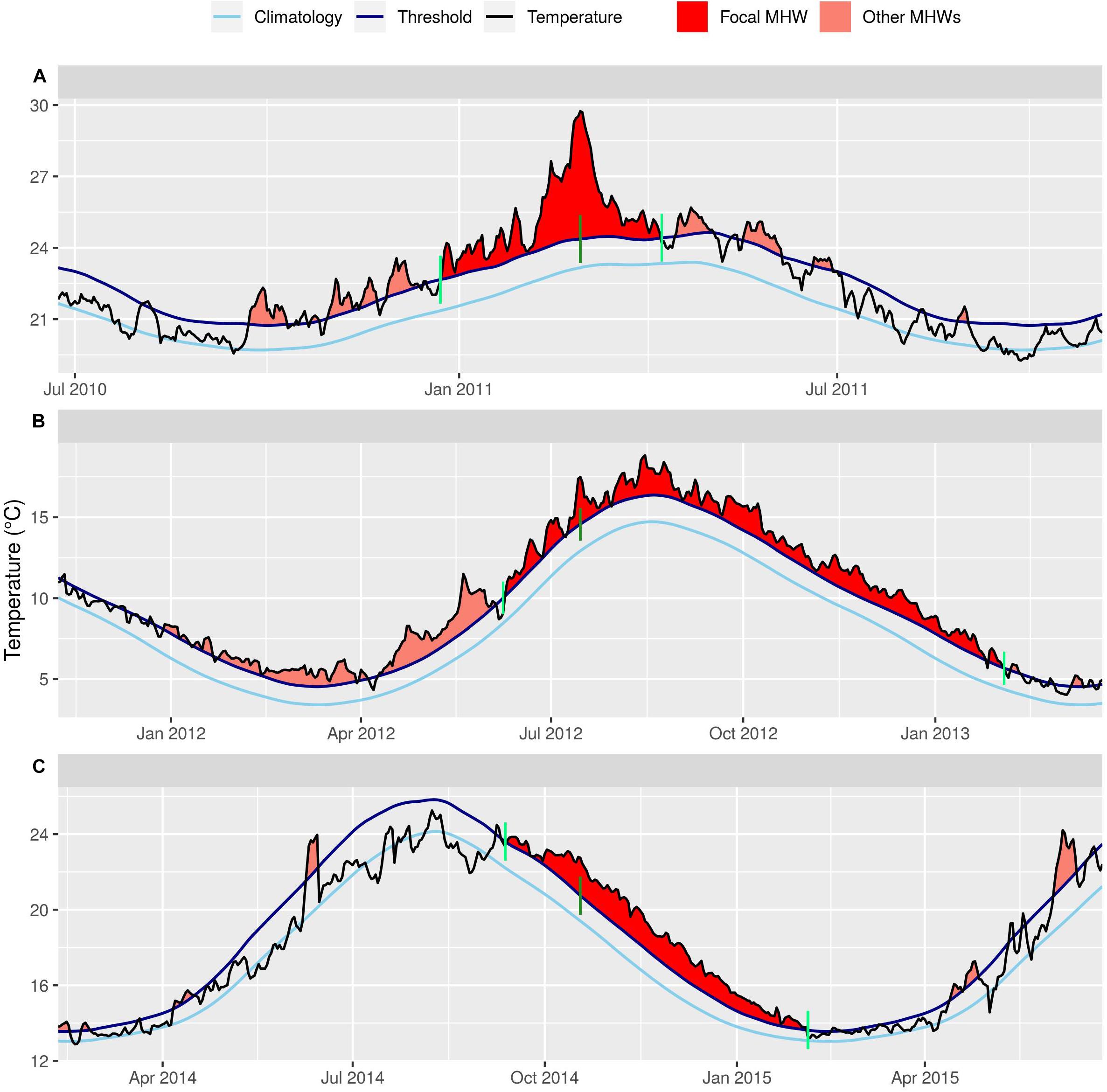
Figure 1. The focal marine heatwaves (MHWs) shown in red for the three reference time series (A) Western Australia (WA), (B) Northwest Atlantic (NWA), and (C) Mediterranean (Med). Other MHWs shown in salmon. Each panel is centered around the peak date of the focal MHW, which is highlighted by a dark green vertical segment. The beginning and end of each MHW are demarcated with light green vertical segments. The seasonal mean climatology for each time series is shown as a light blue line, while the threshold climatology is shown with a dark blue line. The observed temperatures are shown as a black line. Note that only the WA focal MHW is the same as the event in the literature, the focal MHWs shown here for the NWA and Med time series are larger than the MHWs from the literature so are shown here in their stead.

Controlling for Time Series Length

There are currently 37 complete years of data available in the NOAA OISST dataset (1982–2018). In order to determine the effect that time series length has on the output we systematically shorten each time series 1 year at a time from 37 years down to 10 years (2009–2018), before running the MHW detection algorithm. The MHW results for each 1 year step for each of the time series are then compared against the output from the 30 year (1989–2018) version of the same time series as the control.

In order to ensure equitable sample sizes we only compare the MHW metrics for events detected within the last 10 years of each test as this is the period of time during which all of the different tests overlap. This is also why we limited the shortening of the time series lengths to 10 years, so that we would still have a reasonable sample size for all of the other tests.

Because the lengths of the time series were being varied, and were usually less than 30 years in length, it was also necessary that the climatology periods vary likewise. To maintain consistency across the results we use the full range of years within each shortened time series to determine the climatology. For example, if the time series had been shortened from 37 to 32 years (1987–2018), the 32 year period was used to create the climatology. If the shortened time series was 15 years long (2004–2018), this base period was used. The control time series were those with a 30 year length ending in the most recent full year of data available (1989–2018). Note that due to necessity this differs from the suggested climatology period of 1983–2012 that would more closely match the WMO standard (Hobday et al., 2018). The effect of shifting the 30 year climatology base is shown in the Supplementary Figure S2.

The a priori fix proposed to address the issue of short time series length is to use a different climatology estimation technique. The option currently available within the MHW detection algorithm is to expand the window half width used when smoothing the climatology. Other techniques, such as harmonic regression/Fourier analysis, would have a similar effect but are not used here in favor of the (Hobday et al., 2016) method. It is beyond the scope of this paper to compare every possible climatology calculation technique.

Controlling for Missing Data

In order to determine the effect of random missing data on the MHW results, each time series has 0–50% of its data removed in 1% steps before running the MHW algorithm. The control time series are the complete versions.

The a priori fix for missing data in the time series is to linearly interpolate over any gaps. There are many methods of interpolating (imputing) gaps in time series, such as spline interpolation, but we choose linear interpolation here due to its speed, simplicity, and it imposes fewer assumptions on the data. It is beyond the scope of this paper to account for every possible method of interpolation.

Controlling for Long-Term Trend

To quantify the effect of a long-term (secular) trend on the MHW results we add linear trends of 0.00–0.30°C/decade in 0.01°C/decade steps to each time series. The control time series are those with no added trend (e.g., 0.00°C/decade).

There is no proposed a priori method to correct for the added linear trend in these data as this would be simply not to add a trend. Rather it is proposed that the relationship between the slope of the added trend and the effect it has on the results be documented to determine if a predictable relationship may be used for any post hoc corrections.

Results

Time Series Length

Shortening the length of a time series from 30 to 10 years had an unpredictable effect on the count of average MHWs (Figure 2A). At 10 years in length, 90% of the 1000 time series (pixels) tested had between 32% fewer to 85% more MHWs than the 30 year control. The overall increase or decrease in the count of average MHWs was close to linear, meaning that one may be able to say what the change in the count of MHWs may be as a time series is shortened, but it does not allow us to say if this change is positive or negative. The change in the sum of days of the durations of the average MHWs from a 10 year time series ranged from 41% fewer to 84% more than the 30 year control (Figure 2B). This change is slightly more linear than for the count of MHWs, but again, the values may increase or decrease. The mean of the maximum intensities of the average MHWs also either increase or decrease, with 10 year time series having mean maximum intensities anywhere from 16% less to 7% more than the 30 year control.

FIGURE 2

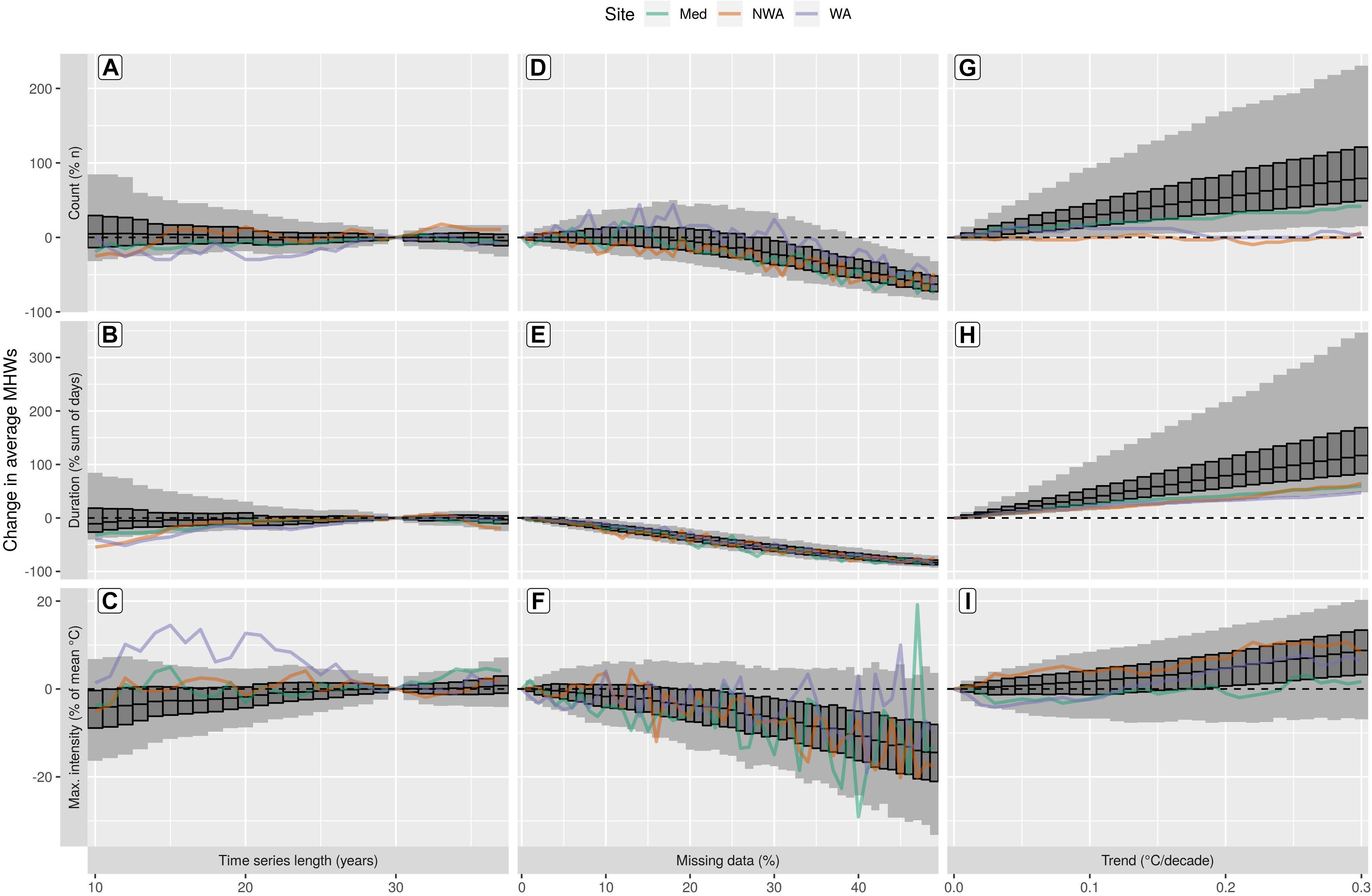
Figure 2. The effects of sub-optimal data on the average MHWs detected in 1000 randomly selected time series (pixels) from the OISST dataset. The columns show the results for each of the three sub-optimal tests: time series length (10–37 years, A–C), missing data (0–50%, D–F), and added long-term trends (0.00–0.30°C/decade, G–I). The rows show the results from the MHW detection output: the percent change in the count of MHWs (A,D,G), the percent change in the sum of the MHW days (B,E,H), and the percent change in the mean of the maximum intensities of the MHWs (C,F,I). The light gray vertical bars show the 5th and 95th quantiles of the values at each step along the x-axis. The dark gray boxplots within the light gray bars show the 25th, 50th, and 75th quantiles of the values at each step. The dashed black line highlights 0 on the y-axis, which denotes where there has been no change from the control time series. The colored lines show the effect of the sub-optimal tests on the three reference time series shown in Figure 1. Note that the x-axes differ between columns, and the y-axes differ between rows.

Increasing the climatology period to more than 30 years had almost as rapid an effect on creating dissimilar results as using fewer years of data. This result stresses the importance of adhering to the WMO standard as closely as possible to ensure the comparability of results (Hobday et al., 2018). It also demonstrates the arbitrariness of the 30 year climatological base period.

Shortening time series length tended to decrease both the duration and maximum intensity of the focal MHW from each time series (Figures 3B,C), while the count of MHWs within the duration of the focal MHW increased (Figure 3A). This is because shortening a time series may increase the seasonal and threshold climatologies, so the shorter a time series becomes, the lower the maximum intensity and shorter the duration of the MHWs may become. MHWs with many spikes (Figure 1A), rather than a smooth hump (Figure 1C), will be particularly affected by this change in the climatology as it will more rapidly break the focal MHW into smaller events (Figure 3A).

FIGURE 3

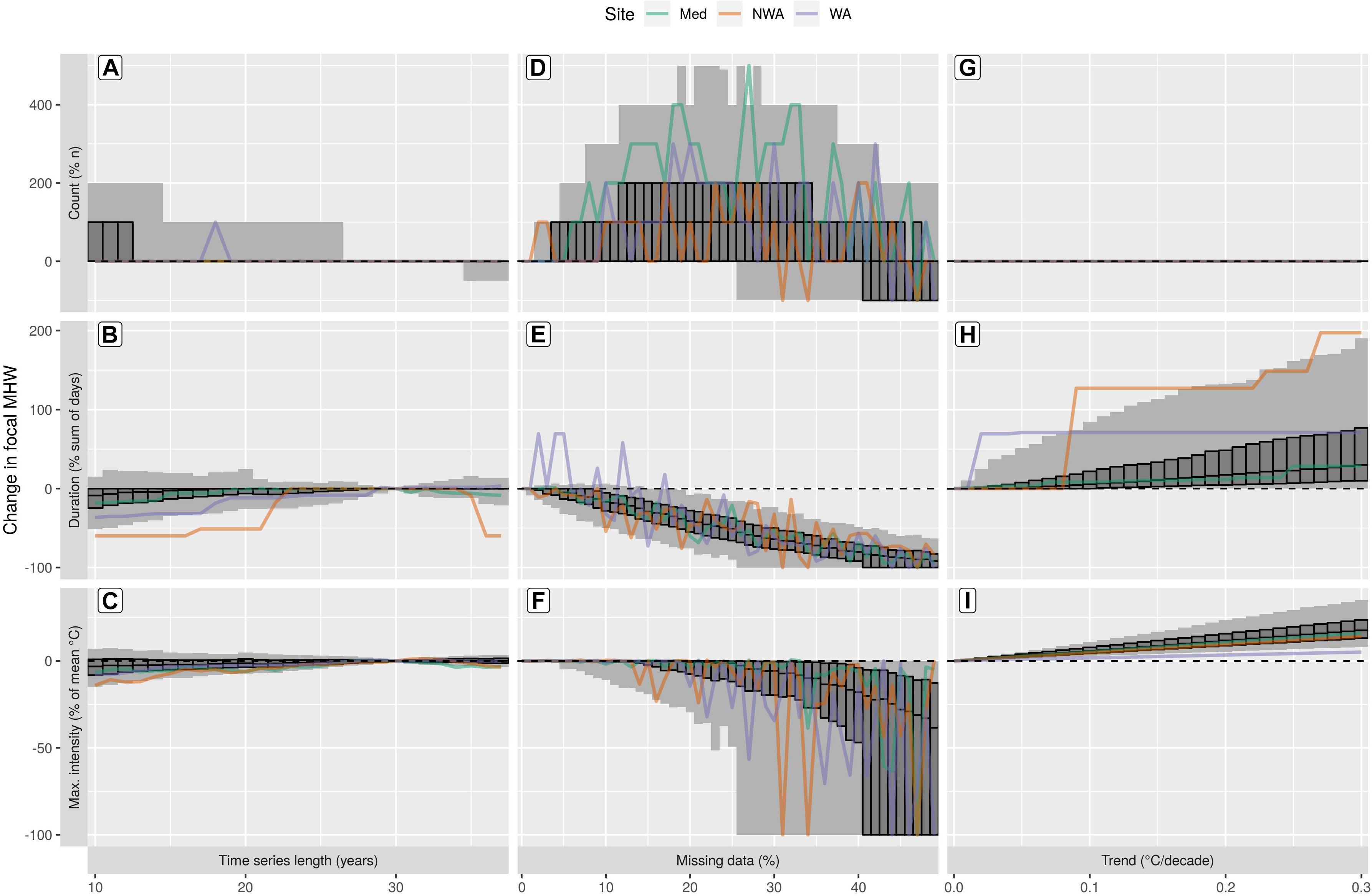
Figure 3. The effects of sub-optimal data on the focal MHWs detected in 1000 randomly selected time series (pixels) from the OISST dataset. The columns and rows of this figure are laid out the same as Figure 2. The top row of panels, “Count (% n)” (A,D,G), shows the difference in the count of MHWs during the duration of the focal event from the control time series. A value of –100% means that no events were detected, and a value of 0% means that no additional MHWs were detected in addition to the focal MHW. Theoretically this value should remain at 0%, when it increases that means that the focal MHW is being broken up into multiple smaller events. The bottom two rows of panels show percentage changes in the duration (B,E,H) and maximum intensity (C,F,I) of the focal MHW. A value of –100% means that no MHW was detected. The 0 line on the y-axis is highlighted with a dashed black line and the effect of the sub-optimal tests on the three reference time series are shown in color.

There are clear global patterns in the changes in MHW results as time series are shortened from 30 to 10 years (Figure 4). The median change in the count of average MHWs due to changes in time series length is only 0.24%/year, but much of the western Pacific and northern Atlantic oceans show large rates of increasing MHW counts as time series are shortened (Figure 4A). The rates of change in the eastern Pacific, southern Atlantic, and the Indian Ocean show a mix of both increasing and decreasing counts of MHWs as time series become shorter. The patterns of change in the sum of MHW days closely resemble the change in the count of MHWs (Figure 4B). The median change in the maximum intensity of average MHWs throughout most of the oceans is −0.21%/year (Figure 4C). This means that, on average, a MHW detected in a 10 year time series will have a maximum intensity about 4.2% cooler than a MHW detected in a 30 year time series (0.21%/year times 20 year difference). This small difference shows the robustness of the MHW detection algorithm. There are areas where decreasing a time series increases the maximum intensities of the MHWs detected. These areas are roughly the same regions where the shortening of a time series causes a decrease in the count of MHW days detected. It is important to note that the long-term trends in these data were removed beforehand so the patterns observed in Figure 4 are due to the properties of the time series themselves and not the climate change signal that would otherwise be dominant in the results.

FIGURE 4

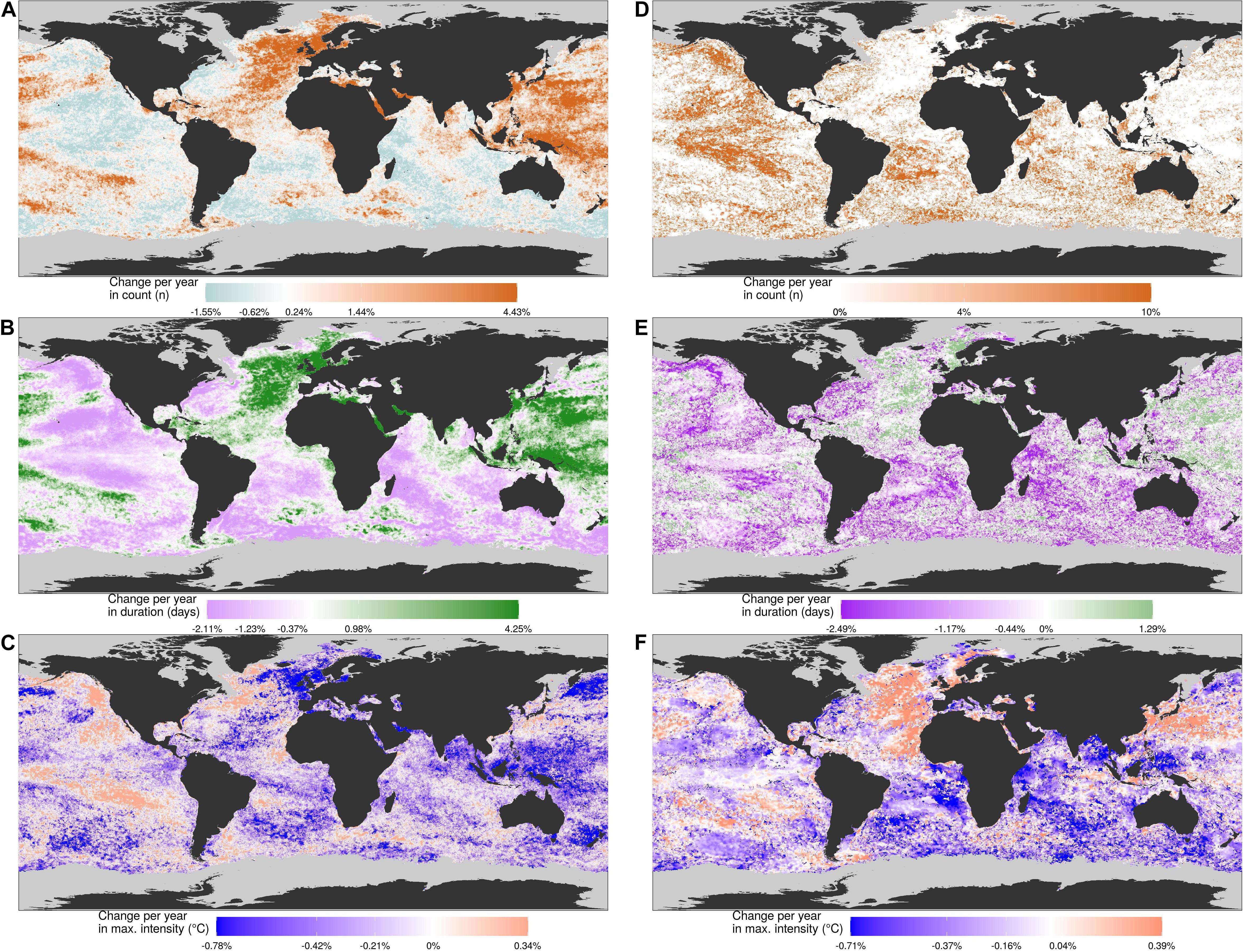
Figure 4. Global map showing changes in MHW detection as the time series at each pixel is shortened from 30 to 10 years. The left column shows the effect of time series length on the average MHWs detected, while the right column shows the effect on the focal MHW. Panels (A,D) show the change in the count of MHWs as the time series are shortened, (B,E) show the change in the duration (days) of the detected MHW(s), and (C,F) show the change in the maximum intensity (°C). The labels on the color bars at the bottom of each panel show what the global values are at the 5th, 25th, 50th, 75th, and 95th quantiles. Any values smaller/larger than the 5th/95th quantile were rounded to prevent the very long tails of the distribution from interfering with the visualization of the results.

The global patterns of the effect of shortened time series on the focal MHWs are similar to the average MHWs. Much of the ocean that shows a decrease in the count of MHWs as a time series is shortened (Figure 4A) also show an increase in the count of MHWs during the duration of the focal MHW at 10% more MHWs per year the time series is shortened (Figure 4D). This may seem contradictory, but this increase in the count of MHWs during the focal MHW in a time series is due to it being broken into smaller events. When this occurs on the smaller MHWs they may be broken up enough to no longer be counted, and therefore the count of average MHWs decreases. The decrease in the durations of the focal MHWs are greater than the decreases for the average MHWs and the spatial homogeneity of this pattern is more broken up (Figures 4B,E). The regions that show increasing durations in the focal MHW are spatially smaller than the average MHWs and the rates of increase are roughly one quarter of those for the average MHWs (Figures 4B,E). Finally, the rates of increase or decrease in maximum intensities were similar in scale between the average and focal MHWs, but differed in their spatial patterns. Whereas the average MHWs show clear warming trends in the northeast and south Pacific (Figure 4C), these features are much reduced for the focal MHWs (Figure 4F). The strong cooling signal in the average MHWs north of Europe is replaced by a spatially broad warming trend in the focal MHWs in the area. The minor warming trend in the average MHWs around the Kuroshio Current is replaced by a spatially larger and more intense warming trend in the focal MHWs.

Missing Data

The effects of increasing missing data on MHW detection were more linear than the effects of time series length, with the exception of MHW count, which was the least linear effect of all tests (Figure 2). Up to 25% missing data, the count of average MHWs in a times series decreases by 45% or increases by 38% (Figure 2D). Past this point the count of MHWs falls at a roughly linear rate until there are 33–86% fewer MHWs when 50% data are missing. The effect of missing data on the sum of the average MHW days was linear at a rate of roughly 2% fewer MHW days in a time series for every 1% of missing data (Figure 2E). The effect of missing data on the maximum intensities of the average MHWs was also linear, but very noisy. The maximum intensities of average MHWs detected in time series missing 50% of their data could decrease by 33% or increase by 3%.

The effect of random missing data on the focal MHW in each time series was dramatic. As missing data in a time series increased, it becomes increasingly likely that the focal MHW is broken into multiple smaller events. It is not uncommon for this to begin with as little as 1% missing data, and increases in severity up to 25–30% (Figure 3D). From this point the number of separate events the MHW is broken into decreases as the smaller events are completely missed due to the loss of data. The duration of the focal MHW was almost always negatively impacted by missing data (Figure 3E). The decrease in duration follows a linear trend of a reduction ranging from 1 to 3% per 1% of missing data. At 26% missing data at least 5% of the time series had their focal MHW removed entirely from the time series, as seen by a reduction in maximum intensity of 100% (Figure 3F). At 41% missing data at least 25% of the time series had their focal MHW removed.

The effect of missing data on a MHW depends largely on their shape, which is the area above the threshold climatology and below the observed anomaly. The WA event has a very pronounced peak (Figure 1A), so when more data are missing it becomes increasingly likely that this peak is not recorded. The maximum intensity measured in the control time series is 6.5°C, but because very few days of this MHW were so intense, increases in missing data become more likely to remove these large values and the maximum intensity of the WA event begins to decrease more rapidly than either the NWA or Mediterranean MHWs. The global patterns in missing data are unremarkable and generally consistent across the oceans (Supplementary Figure S3).

Long-Term Trend

The effect of a long-term trend on MHW detection was the most linear of the three tests and resulted in the largest changes in the results. An added linear trend can lead to a reduction in the count of average MHWs in a time series, but generally it causes a linear increase at roughly 3% additional average MHWs detected for every 0.01°C/decade added (Figure 2G). The effect that these additional MHWs had on the sum of average MHW days was an increase, ranging from 1.7 to 11.5% for every 0.01°C/decade added (Figure 2H). This means that the average MHWs detected in a time series with a long-term trend of 0.30°C/decade could be 48–347% longer than in the same time series with no long-term trend. The effect of linear trends on the maximum intensity of the average MHWs, though generally linear, could be either positive or negative at a rate of −0.1–0.6% per 0.01°C/decade added.

The focal MHW in each time series was never broken into multiple events due to the added long-term trend (Figure 3G), however, the duration of the focal MHWs were affected differently. The Mediterranean MHW showed practically no increase in duration due to an added long-term trend, the WA MHW saw a large jump at 0.03°C/decade, and the NWA MHW had a dramatic jump at an added trend of 0.09°C/decade, followed by a few other increases at larger added trends (Figure 3H). Likewise, all of the other 1000 time series included in Figure 3 tend to jump up in dramatic steps, as seen by the very large range in the 90 and 50% confidence intervals (CI). These jumps in duration occur as the temperature anomalies increase more rapidly than the threshold and neighboring MHWs in a time series connect into one event. The effect that the long-term trend had on the maximum intensity of focal MHWs was also linear and at an added trend of 0.30°C/decade the 90% CI was from 8 to 35% of the control value (Figure 3I). The global patterns in added long-term trends generally show that MHW metrics increase (Supplementary Figure S4).

Best Practices

Given the effect of time series length, missing data, and long-term trends on the detection of MHWs, we can quantify the uncertainty in the results when using sub-optimal data. In Table 1 the increasing rates of uncertainty per step in the sub-optimal tests for average MHWs is shown, while Table 2 shows the uncertainty for the focal MHWs. For example, a time series that is 20 years in length (10 years shorter than optimal), will result in a median difference in the duration of average MHWs that is 3% lower, and the 90% CI will be ±27% around that median difference. These rates of uncertainty at the 90% CI are large, but knowing where in the world a time series comes from it is possible to make a more accurate inference. For example, the change in the duration of average MHWs in the North Sea as the time series are shortened is very consistently positive and near the high end of the global distribution (Figure 4B). This means that one can be more confident that the upper range of the 90% CI is an appropriate choice when estimating the possible change in results if they had been calculated with an optimal time series (30 years). One final point of consideration in the application of this information for judging uncertainty is to consider how linear the response of the results to the sub-optimal tests is. The values in parentheses in Tables 1, 2 show the R² (coefficient of determination) for each linear model that was used to determine the change in uncertainty as time series become more sub-optimal. More examples, as well as a step-by-step walk through for how to use the numbers in these tables, are provided in each sub-section below. The a priori and post hoc fixes proposed in the methods are also covered in more detail in the following sub-sections. It must be stressed here that the methods proposed below for working with sub-optimal data do not address the issues that remotely sensed data have near coastlines.

TABLE 1

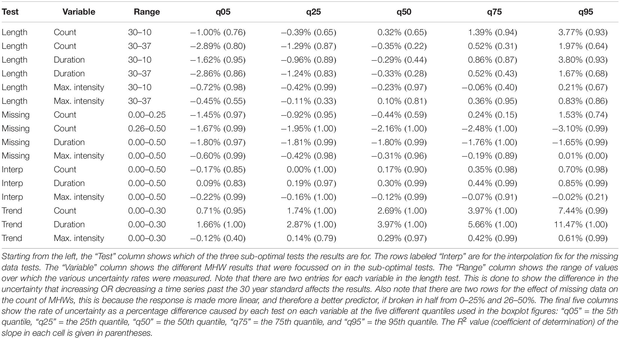
Table 1. The degree of uncertainty introduced into the average marine heatwave (MHW) results as time series become increasingly sub-optimal.

TABLE 2

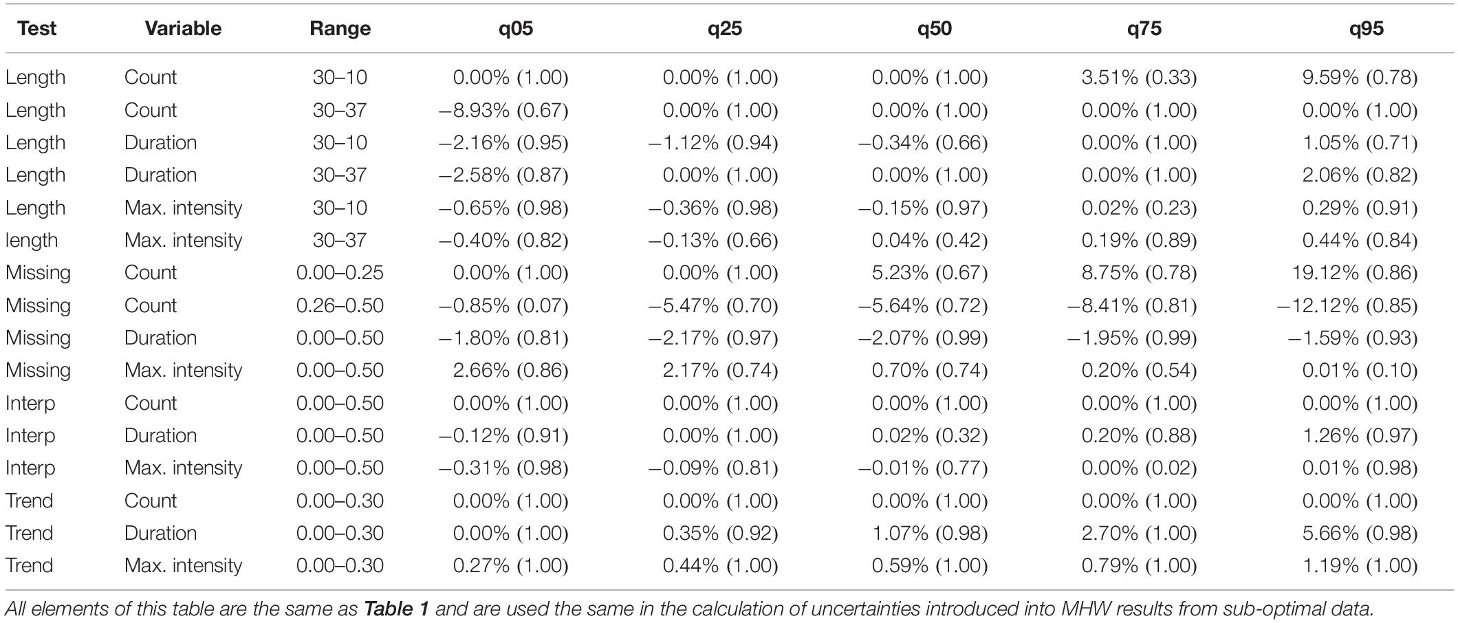
Table 2. The degree of uncertainty introduced into the focal marine heatwave (MHW) results as time series become increasingly sub-optimal.

Correcting for Time Series Length

The a priori fix proposed for shorter time series, creating a smoother seasonal signal by expanding the window half-width of the moving average, was not a reliable option and this should be left as the standard 5 day period. Increasing the window half-width to as much as 30 days has very little effect on the 50% (interquartile) and 90% CI ranges for the count of average MHWs, the effect on individual time series is inconsistent (Figure 5, top row). The effect of this change to the detection algorithm on the duration of average MHWs was negligible at all window half-widths tested (Figure 5, middle row). The effect of wider window half-widths on the maximum intensity of the average MHWs appeared to help keep the results comparable (Figure 5, bottom row), but upon closer inspection this was found to be misleading. The effect of widening the window half-widths was similar for the results of the focal MHWs (Supplementary Figure S5). The widening of the window half-widths affects MHW detection by flattening the shape of the sinusoidal seasonal climatology. The overall mean value does not change, but the peaks and troughs are pulled closer to the mean while the slopes between them become more gradual. Because the mean of the seasonal signal does not change, the total anomalous observations remain similar, but where along the seasonal signal those anomalies are detected may shift dramatically. This is particularly noticeable for MHWs that occur at the peak of summer because the seasonal and threshold climatologies are lowered the most here, making these events appear more intense.

FIGURE 5

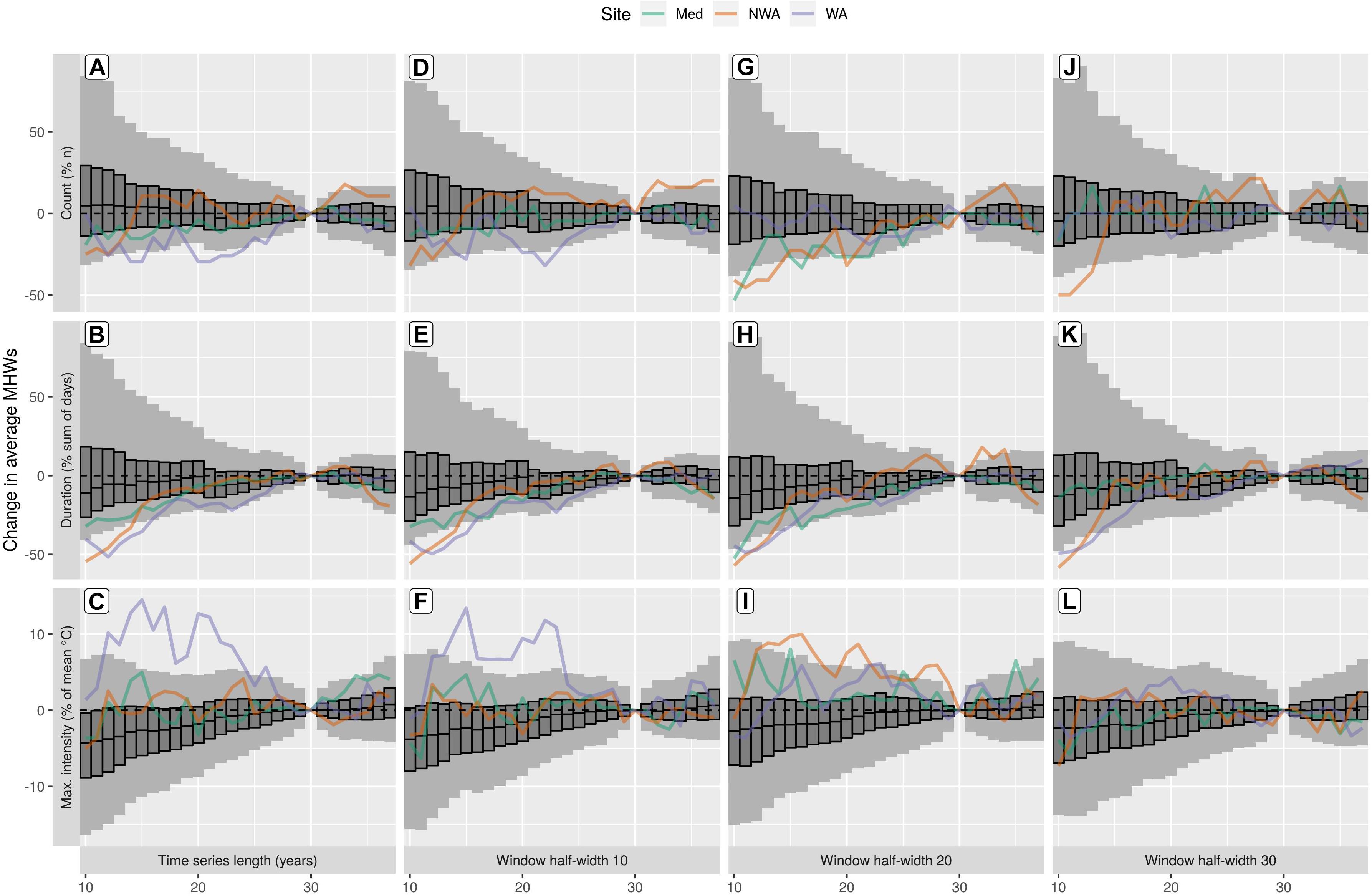
Figure 5. The effect of changing the window half-widths used for seasonal and threshold climatology creation on average MHW detection. The left column (A–C) is reproduced from Figures 2A–C and included here for ease of comparison to the effects of the three different window half-widths tested: 10 (D–F), 20 (G–I), and 30 (J–L) days. The default window half-width of 5 days is used in the left column. All other elements are the same as Figures 2, 3.

Although an a priori fix for time series length is not effective, the known rates of uncertainty can be used to provide the post hoc uncertainty to detected MHWs. Using the focal MHW uncertainty rates as an example, the first six rows of Table 2 show the rate of uncertainty introduced into results for a focal MHW for each year less or more than 30 years. The “Range” column in Tables 1, 2 indicate which direction from the 30 year control the slope in uncertainty is moving. The focal MHW detected in a 10 year time series will have a median (50th quantile) difference in maximum intensity of −3% from that same MHW in a 30 year time series (Table 2, row 5, column “q50,” value = −0.15%/year shorter than 30). This may be estimated by taking the value found in the corresponding cell of the table and multiplying it by the number of years that the time series is shorter (or longer) than the 30 year optimal length. It is unlikely that results will match the median difference. It is more likely that the detected MHW will fall somewhere within the 50% CI (Tables 1, 2, column “q25” to “q75”), or the 90% CI (Tables 1, 2, column “q05” to “q95”) range. To determine these ranges in uncertainty, an approach is to use the slope found in the respective columns and multiply each slope by the number of years that the time series is shorter or longer than the 30 year control. This provides the full range of uncertainty within the 50% CI or 90% CI as well as the median change. For example, the 50% CI in the change in the maximum intensity of a focal MHW in a 10 year time series is found by multiplying the 25th and 75th quantiles of change. Using the 10 year time series example described above, this means that the overall range of uncertainty around the median change is: 0.38% × 20 (difference in years) = 7.6%, the change in the 25th quantile is −0.36% × 20 = −7.2%, and the change in the 75th percentile is 0.02% × 20 = 0.4%. The final estimate of the 50 CI around the median change in maximum intensity is therefore: −7.2, −3.8, and 0.4%. This means that in a 10 year time series one can assume that the focal MHW detected has a 50% chance of having a maximum intensity that is somewhere between −7.2 and 0.4% of the same MHW estimated using a 30 year times series.

Correcting for Missing Data

Linear interpolation was proposed as an a priori fix to address the issue of missing data and was effective. This fix could allow the use of time series missing more than 50% of their data (Figure 6), assuming that there is not so much missing data that the period of time during a MHW is completely missing. The rates of uncertainty that missing data introduce into detected MHWs may be found in rows 7–10 of Tables 1, 2, but we will focus on the use of the rates of uncertainty for interpolated data here as this is an effective fix. Note that rows 7 and 8 of Tables 1, 2 show rates of change in the count of MHWs for missing data between different ranges of missing data. This is because the change in the count of MHWs due to missing data is not linear. If one cuts the data at roughly 25% this provides the highest R² values for the two slopes (most linear fit).

FIGURE 6

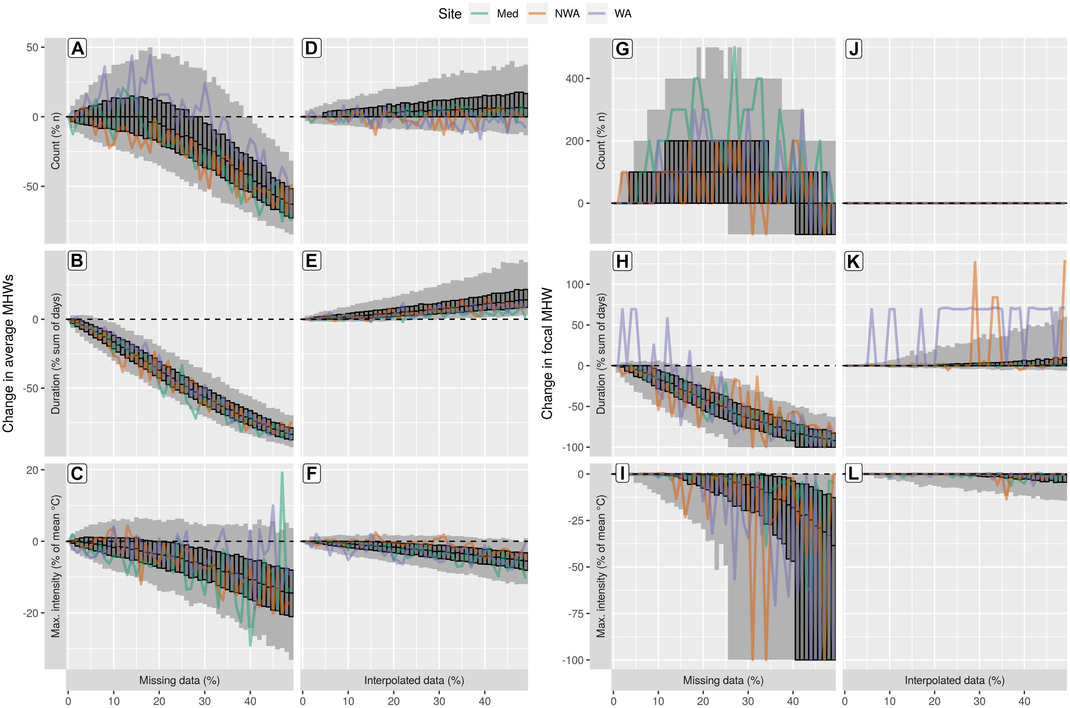
Figure 6. The effect of linear interpolation on the MHW results from time series with missing data. The left column (A–C) and centre-right column (G–I) are reproduced from Figures 2D–F and Figures 3D–F respectively. They are included here for convenience of comparison against the columns that show the results of linearly interpolating missing data before detecting average MHWs (D–F) and focal MHWs (J–L). Note that the y-axes of the left two columns are not the same as the right two columns. A value of –100% along the y-axis means no MHWs were detected. All other elements are the same as Figures 2, 3, and 5.

As an example for the use of linear interpolation over missing data in a time series we show how to calculate the 90% CI around the average MHW duration in a time series missing 30% data. The median rate of change in average MHW duration per 1% missing data after linear interpolation is 0.3% (Table 1, row 12, column “q50”), the rate of change for the 5th quantile is 0.09% (Table 1, row 12, column “q05”), and for the 95th quantile it is 0.85% (Table 1, row 12, column “q95”). At 30% linearly interpolated data one may assume a 90% CI around the average MHW duration to be 2.7% – 9.0% – 25.5%. In other words, there is a 90% chance that the average duration of the MHWs detected in a time series with 30% interpolated data are between 2.7 and 25.5% that of the MHWs detected in the same time series without any missing data.

Correcting for Long-Term Trend

There was no a priori fix proposed for the correction of an added linear trend. Rather, by knowing the trend in a time series a priori we have been able to model the effect that it has on detected MHWs. The effect that long-term trends have on the results are much greater than for time series length or missing data, and the effects are more linear, therefore; we can be more confident in the uncertainty we assign to the detected MHWs. However, the ranges of uncertainty introduced by long-term trends are also much greater than for the other two tests. To illustrate how long-term trends affect the count of average MHWs we use a time series with a known linear trend of 0.25°C/decade. The median rate at which a long-term trend in a time series affects the count of average MHWs is 2.69% per 0.01°C/decade (Table 1, row 14, column “q50”), the 5th quantile is 0.71% (Table 1, row 14, column “q05”), and the 95th quantile is 7.44% (Table 1, row 14, column “q95”), therefore; the count of average MHWs detected in a time series with a long-term trend of 0.25°C/decade is likely (90% CI) 17.75% – 67.25% – 186%. This is a very large effect that supports the argument for using a 10 year long or 50% interpolated data time series. There are long-term trends present in most time series being used and these effects on the MHWs therein are almost certainly greater than using short time series with missing data. If one is comfortable detecting MHWs in a time series before detrending it, one should be comfortable with the use of time series shorter than 30 years or missing some data.

Discussion

This investigation into the effects of sub-optimal data on MHW detection revealed that there are no clear statistical thresholds at which the outputs of the MHW algorithm diverge from optimal data. The ranges of uncertainty that sub-optimal data introduce into MHW results could be determined and users may now decide their acceptable level of uncertainty. It must be noted that having used only SST data for these investigations the results may not accurately represent the properties of sub-surface MHWs, which may last longer and be more intense than those at the surface (Schaeffer and Roughan, 2017; Darmaraki et al., 2019).

The MHW results from time series with 10 years of data are not appreciably different from the MHWs detected with 30 years of data. The rates at which the count, duration, and maximum intensity of MHW change from year-to-year within a single time series may vary wildly, but a global sampling showed that the increasing range in the uncertainty of the results one may expect are roughly linear. The rates of uncertainty in Table 1 may therefore be applied post hoc to MHWs detected in shorter time series to provide the uncertainly range within which the results are comparable to those from an optimal time series.

An unexpected result was that increasing the base period used for climatology creation to longer than 30 years reduced the probability that the outputs would be comparable by as much as shortening the base period did. This means that the common (often unspoken) assumption that using 30 years of data is the same as using >30 years of data for a base period is incorrect. In other words, a 30 year time series is often thought of as the minimum length needed to constrain the climatology but we have shown here that using a climatology period greater than 30 years may create outputs as different as using fewer than 30 years. This is due to the decadal and multi-decadal variability in an environmental time series. In time series with less decadal to multi-decadal variability there will be no appreciable difference between results calculated with a 30 year base period versus the 30+ years. In a time series with large decadal to multi-decadal variability, a base period of 30 years is not long enough to remove this variability. It is therefore important to stress the adherence to the WMO standards for climatology periods as closely as possible to ensure results are comparable to other studies (Hobday et al., 2018). Increased smoothing of the climatologies derived from shortened time series was not an effective fix so it is recommend that the default climatology method in Hobday et al. (2016) also be followed to maximize comparability between studies.

The MHW algorithm proved to be resilient to missing data. Time series missing up to 25% of their data resulted in a count of MHWs comparable to using a 10 year time series and the rate of increase in uncertainty can be modeled with some accuracy. Time series missing more than 25% were affected too much and too unpredictably for the results to be reliable, while focal MHWs were sometimes not detected with 26% or more missing data. Fortunately, the effect that missing data has on the duration of average MHWs in a time series is predictable and can be corrected (Table 1). A simple correction for missing data in a time series is to linearly interpolate over the gaps – for more than 50% missing data, the results will have less uncertainty in them than using a 10 year time series. This advice assumes that missing data is distributed through the time series, if the period of time during a MHW is missing large sections of data, interpolation will not be effective.

The long-term temperature trends in times series have the largest potential effect on the MHWs detected. These effects are the most predictable of the three issues examined but also introduce the largest ranges of uncertainty. The increase in duration from added long-term trends led to temperatures in the time series usually increasing “faster” than the 90th percentile threshold. So as the slope of the added trend increases, the length of a given MHW increases. MHWs with a slow onset/decline (e.g., the NWA event) will increase in duration more rapidly, while those with a more rapid onset/decline (e.g., the Mediterranean event) will not appreciably change in duration with a larger long-term trend. A series of MHWs separated by short periods of time may merge into a single larger event (e.g., the WA event). This reduces the overall count of the MHWs detected in a time series while increasing the mean duration of the events detected.

Conclusion

The acceptable sub-optimal data limits, their proposed corrections, and the amount of uncertainty they introduce into the results are as follows:

(1) Time series length:

• A length of 10 years produces acceptable MHW metrics that may be used with some caution.

• Smoothing the climatology before detecting MHWs does not improve the results and should not be done.

• The largest uncertainty that shorter time series introduce into average or focal MHWs is duration:

• Average MHW duration changes by −1.62–3.8%/year shorter than 30 (90% CI).

• Focal MHW duration changes by −2.16–1.05%/year shorter than 30 (90% CI).

(2) Missing data:

• The effect of missing data up to 25% on MHW results is comparable to the effect of a 10 year time series.

• Focal MHWs may begin to disappear from time series missing 26% or more data.

• Linear interpolation is an excellent fix for missing data up to 50%, assuming that the time period of interest is not completely missing.

• The largest uncertainty that linearly interpolated missing data introduce into MHW results is duration:

• Average MHW duration changes by 0.09–0.85% per% interpolated (90% CI).

• Focal MHW duration changes by −0.12–1.26% per% interpolated (90% CI).

(3) Long-term trends.

• Long-term trends had the greatest effect on MHWs of the three sub-optimal tests and had the greatest range of uncertainty around those effects.

• Long-term trends in excess of those tested in this paper occur naturally and are rarely controlled for so no limit is proposed here.

• The duration of MHWs is what is affected most by a long term trend in the data:

• Average MHW duration changes by 1.66–11.47% per 0.01°C/decade (90% CI).

• Focal MHW duration changes by 0.00–5.66% per 0.01°C/decade (90% CI).

Researchers need not avoid using sub-optimal time series, such as might be the best available for coastal research or sub-surface analyses. Time series length may have an unpredictable effect on MHW results, but this may be corrected, and time series lengths as short as 10 years are still useful for MHW research. Missing data has a larger effect on MHW detection, but linear interpolation can compensate for up to 50% missing data. Lastly, the effect of long-term trends on MHW detection are the largest and most linear but also have the largest uncertainties. The MHW detection algorithm is robust and researchers may be confident in the inter-comparability of results when using time series within a generous range of sub-optimal data challenges.

Data Availability Statement

The code and datasets generated for this study may be found at https://github.com/robwschlegel/MHWdetection. A detailed outline of the code used in this methodology may be found at https://robwschlegel.github.io/MHWdetection/.

Author Contributions

RS prepared the majority of the text, figures, synthesized the comments, and uploaded the manuscript. AS prepared a large portion of an early version of the text and a number of initial figures. AH, EO, and AS provided several rounds of comments on the manuscript as it was developed.

Funding

This research was supported by the Ocean Frontier Institute through an award from the Canada First Research Excellence Fund. Funding was also provided through the National Sciences and Engineering Research Council of Canada Discovery Grant RGPIN-2018-05255.

Conflict of Interest

The authors declare that the research was conducted in the absence of any commercial or financial relationships that could be construed as a potential conflict of interest.

Acknowledgments

The authors would like to acknowledge the contributions of the reviewers in the development of this manuscript.

Supplementary Material

The Supplementary Material for this article can be found online at: https://www.frontiersin.org/articles/10.3389/fmars.2019.00737/full#supplementary-material

Footnotes

1. ^ http://www.marineheatwaves.org/
2. ^ https://github.com/ecjoliver/marineHeatWaves

References

Banzon, V., Smith, T. M., Chin, T. M., Liu, C., and Hankins, W. (2016). A long-term record of blended satellite and in situ sea-surface temperature for climate monitoring, modeling and environmental studies. Earth Syst. Sci. Data 8, 165–176. doi: 10.5194/essd-8-165-2016

CrossRef Full Text | Google Scholar

Baumgartner, T. R. (1992). Reconstruction of the history of the pacific sardine and northern anchovy populations over the past two millenia from sediments of the Santa Barbara basin, California. CalCOFI Rep. 33, 24–40.

Google Scholar

Darmaraki, S., Somot, S., Sevault, F., and Nabat, P. (2019). Past variability of Mediterranean Sea marine heatwaves. Geophys. Res. Lett. 46, 9813–9823. doi: 10.1029/2019GL082933

CrossRef Full Text | Google Scholar

Dayton, P. K., Tegner, M. J., Parnell, P. E., and Edwards, P. B. (1992). Temporal and spatial patterns of disturbance and recovery in a kelp forest community. Ecol. Monogr. 62, 421–445. doi: 10.2307/2937118

CrossRef Full Text | Google Scholar

Fordyce, A. J., Ainsworth, T. D., Heron, S. F., and Leggat, W. (2019). Marine heatwave hotspots in coral reef environments: physical drivers, ecophysiological outcomes and impact upon structural complexity. Front. Mar. Sci. 6:498. doi: 10.3389/fmars.2019.00498

CrossRef Full Text | Google Scholar

Garrabou, J., Coma, R., Bensoussan, N., Bally, M., Chevaldonné, P., Cigliano, M., et al. (2009). Mass mortality in Northwestern Mediterranean rocky benthic communities: effects of the 2003 heat wave. Glob. Change Biol. 15, 1090–1103. doi: 10.1111/j.1365-2486.2008.01823.x

CrossRef Full Text | Google Scholar

Harrison, B., Jupp, D., Lewis, M., Forster, B., Mueller, N., Smith, C., et al. (2019). Earth Observation: Data, Processing and Applications. Melbourne, VIC: Australia and New Zealand CRC for Spatial Information.

Google Scholar

Hobday, A. J., Alexander, L. V., Perkins, S. E., Smale, D. A., Straub, S. C., Oliver, E. C. J., et al. (2016). A hierarchical approach to defining marine heatwaves. Progr. Oceanogr. 141, 227–238. doi: 10.1016/j.pocean.2015.12.014

CrossRef Full Text | Google Scholar

Hobday, A. J., Oliver, E. C. J., Gupta, A. S., Benthuysen, J. A., Burrows, M. T., Donat, M. G., et al. (2018). Categorizing and naming marine heatwaves. Oceanography 31, 162–173. doi: 10.5670/oceanog.2018.5205

CrossRef Full Text | Google Scholar

Mills, K., Pershing, A., Brown, C., Chen, Y., Chiang, F. S., Holland, D., et al. (2013). Fisheries management in a changing climate: lessons from the 2012 ocean heat wave in the Northwest Atlantic. Oceanography 26, 191–195. doi: 10.5670/oceanog.2013.27

CrossRef Full Text | Google Scholar

Oliver, E. C. J., Donat, M. G., Burrows, M. T., Moore, P. J., Smale, D. A., Alexander, L. V., et al. (2018). Longer and more frequent marine heatwaves over the past century. Nat. commun. 9:1324. doi: 10.1038/s41467-018-03732-9

PubMed Abstract | CrossRef Full Text | Google Scholar

Oliver, E. C. J., Lago, V., Holbrook, N. J., Ling, S. D., Mundy, C. N., and Hobday, A. J. (2017). Eastern Tasmania Marine Heatwave Atlas, Institute for Marine and Antarctic Studies. Hobart, TAS: University of Tasmania, doi: 10.4226/77/587e97d9b2bf9

CrossRef Full Text | Google Scholar

Pachauri, R. K., Allen, M. R., Barros, V. R., Broome, J., Cramer, W., Christ, R., et al. (2014). Synthesis Report. Contribution of Working Groups i, ii and iii to the Fifth Assessment Report of The Intergovernmental Panel on Climate Change. Climate Change 2014. (Geneva: Intergovernmental Panel on Climate Change)Google Scholar

Philander, S. G. H. (1983). El nino southern oscillation phenomena. Nature 302:295. doi: 10.1038/302295a0

CrossRef Full Text | Google Scholar

Reynolds, R. W., Smith, T. M., Liu, C., Chelton, D. B., Casey, K. S., and Schlax, M. G. (2007). Daily high-resolution-blended analyses for sea surface temperature. J. Clim. 20, 5473–5496. doi: 10.1175/2007JCLI1824.1

CrossRef Full Text | Google Scholar

Salinger, J., Hobday, A., Matear, R., O’Kane, T., Risbey, J., Dunstan, P., et al. (2016). “Chapter one - decadal-scale forecasting of climate drivers for marine applications,” in Advances in Marine Biology, ed. B. E. Curry (Cambridge, MA: Academic Press), 1–68. doi: 10.1016/bs.amb.2016.04.002

PubMed Abstract | CrossRef Full Text | Google Scholar

Schaeffer, A., and Roughan, M. (2017). Sub-surface intensification of marine heatwaves off southeastern Australia: the role of stratification and local winds. Geophy. Res. Lett. 44, 5025–5033. doi: 10.1002/2017GL073714

CrossRef Full Text | Google Scholar

Schlegel, R. W., and Smit, A. J. (2018). heatwaveR: a central algorithm for the detection of heatwaves and cold-spells. J. Open Sour. Softw. 3:821. doi: 10.21105/joss.00821

CrossRef Full Text | Google Scholar

Smale, D. A., and Wernberg, T. (2009). Satellite-derived SST data as a proxy for water temperature in nearshore benthic ecology. Mar. Ecol. Prog. Ser. 387, 27–37. doi: 10.3354/meps08132

CrossRef Full Text | Google Scholar

Smale, D. A., Wernberg, T., Oliver, E. C. J., Thomsen, M., Harvey, B. P., Straub, S. C., et al. (2019). Marine heatwaves threaten global biodiversity and the provision of ecosystem services. Nat. Clim. Change 9, 306–312. doi: 10.1038/s41558-019-0412-1

CrossRef Full Text | Google Scholar

Smit, A. J., Roberts, M., Anderson, R. J., Dufois, F., Dudley, S. F. J., Bornman, T. G., et al. (2013). A coastal seawater temperature dataset for biogeographical studies: large biases between in situ and remotely-sensed data sets around the coast of South Africa. PLoS One 8:e81944. doi: 10.1371/journal.pone.0081944

PubMed Abstract | CrossRef Full Text | Google Scholar

Stobart, B., Mayfield, S., Mundy, C., Hobday, A., and Hartog, J. (2016). Comparison of in situ and satellite sea surface-temperature data from south Australia and Tasmania: how reliable are satellite data as a proxy for coastal temperatures in temperate southern Australia? Mar. Freshw. Res. 67, 612–625. doi: 10.1071/MF14340

CrossRef Full Text | Google Scholar

Wernberg, T., Smale, D. A., Tuya, F., Thomsen, M. S., Langlois, T. J., de Bettignies, T., et al. (2012). An extreme climatic event alters marine ecosystem structure in a global biodiversity hotspot. Nat. Clim. Change 3, 78–82. doi: 10.1038/nclimate1627

CrossRef Full Text | Google Scholar

WMO, (2011). Guide to Climatological Practices. Geneva: World Meteorological Organization.

Google Scholar

WMO, (2017). WMO Guidelines on the Calculation of Climate Normals. Geneva: World Meteorological Organization.

Google Scholar

Zhao, Z., and Marin, M. (2019). A MATLAB toolbox to detect and analyze marine heatwaves. J. Open Source Softw. 4:1124. doi: 10.21105/joss.01124

CrossRef Full Text | Google Scholar