Hotter and Weaker Mediterranean Outflow as a Response to Basin-Wide Alterations

Introduction

The Mediterranean Sea (MedSea hereinafter) is the only basin away from polar regions where open-ocean deep convection reaching the ocean bottom happens, despite its location in temperate latitudes. The convection is the result of the net buoyancy flux to the atmosphere, mainly determined by the fresh water deficit (evaporation minus precipitation and river runoff, E-P) of the basin. It drives an open thermohaline circulation cell starting and ending in the Strait of Gibraltar (SoG, hereinafter), the only relevant connection of the MedSea with the open ocean. The cell starts with a surface inflow of Atlantic water that travels the whole Mediterranean Sea to be transformed into the very salty Levantine Intermediate Water (LIW) in the easternmost basin of the MedSea (Figure 1). There, it sinks and initiates the way back to the SoG and to the open ocean as a dense underflow, thus completing the thermohaline cell (see Hopkins (1985) or Tsimplis et al. (2006), for instance, for a review on this general topic).

FIGURE 1

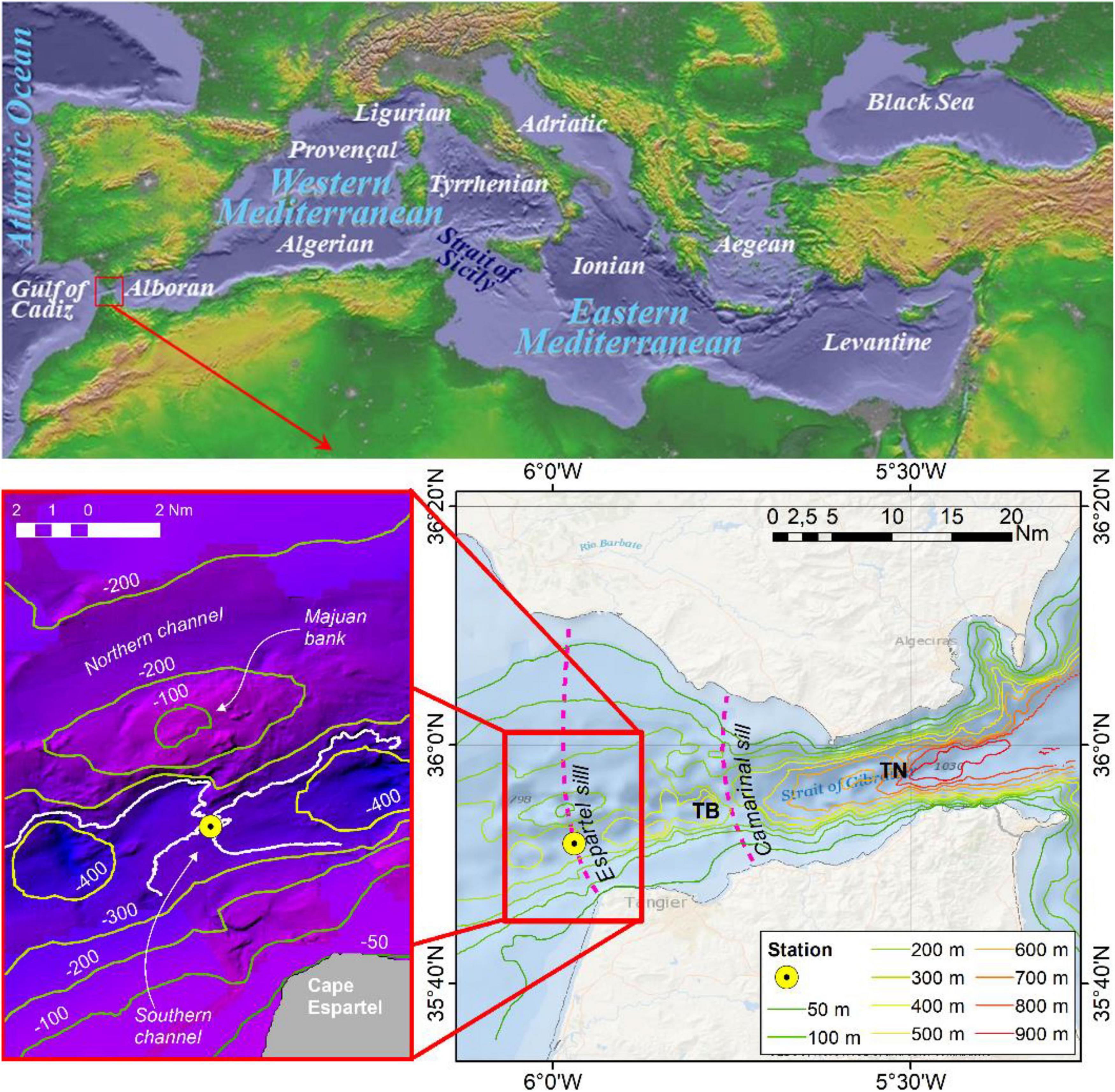
Figure 1. Top panel. Map of the Mediterranean Sea with the name of the main basins and sub-basins. Red rectangle indicates the area of the Strait of Gibraltar enlarged below. Bottom-right panel: map of the Strait with indication of relevant topographic features. TN stands for Tarifa Narrows; TB, for Tangier Basin. Red rectangle indicates the zone of Espartel sill enlarged in the bottom-left panel. Yellow dot indicates the location of the monitoring station. Most of the Mediterranean outflow goes along the channel between Majuan bank and the African shore (Sánchez-Román et al., 2009; Sammartino et al., 2015).

In addition to intermediate waters, deep waters are formed in different places of the MedSea, mainly in the Adriatic and Aegean Seas in the eastern basin (Eastern Mediterranean Deep Water, EMDW; Schlitzer et al., 1991; Roether et al., 1996), and in the Gulf of Lions in the western basin (Western Mediterranean Deep Water, WMDW; Stommel, 1972). The basic thermohaline cell becomes more complex since both basins have their own closed thermohaline circulations (Tsimplis et al., 2006) and bottom water renewal processes. The EMDW is mainly renewed by upwelling inside the eastern basin itself (Schlitzer et al., 1991; Roether and Schlitzer, 1991) and only a very small fraction seems to be drained out to the western basin through the Sicily Strait (Astraldi et al., 1999). On the contrary, a significant fraction of WMDW finds its way out to the Atlantic Ocean through the SoG (Stommel et al., 1973; Kinder and Parrilla, 1987), even though the depth of the SoG’s main sill (Camarinal sill, 290m, Figure 1) is less than Sicily’s west and east sills (360m and 430m, respectively, Astraldi et al., 1999). Bernoulli aspiration of WMDW in the Alboran Sea by the energetic lower layer flow at the SoG (Bryden and Stommel, 1982; Naranjo et al., 2012) is responsible for the differentiated pattern of both basins, as the Strait of Sicily does not hold any comparable bottom current.

Levantine Intermediate Water and WMDW make up the main bulk of the Mediterranean outflow in the SoG (Q₂ hereinafter, assumed negative as it flows westwards), to which small fractions of other intermediate and deep waters may eventually contribute (Naranjo et al., 2015). The Mediterranean outflow has to flow out beneath a slightly greater Atlantic inflow (Q₁, positive), moving over a very irregular seafloor with steep sills and marked contractions (Figure 1). This strongly constraining topography leads to hydraulic control of the exchanged flows, an idea first suggested by Bryden and Stommel (1984) and further addressed by Armi and Farmer (1985). A relevant result of this theory is that the exchanged flows attain a maximum value that cannot be exceeded whenever the exchange is hydraulically controlled (maximal exchange, Armi and Farmer, 1985, 1987). In other words, |Q₂| has an upper limit. From this point of view, the two-layer hydraulic theory provides a useful frame to interpret the observations collected at Espartel sill (Figure 1), the westernmost sill of the SoG, which constitute the dataset analyzed and exploited in the present study. Next Section revises some relevant aspects of this theory applied to the SoG.

The Hydraulically-Controlled Exchange Model

The objective of this work is to infer changes in the MedSea from single-point observations at the site where it joins with the global ocean (Figure 1). Within the frame of two-layer theory, the usual approach is to consider the MedSea as a homogeneous basin connected to the Atlantic Ocean, also homogeneous, through a channel (the SoG). Actually, the outflow consists of different water masses of very similar density, which justifies homogeneity for dynamic purposes as a first order approach. The approach, however, cannot be applied to the water masses analysis carried out later on.

The simplest model for the SoG is a non-rotating channel of rectangular section with no mixing between layers (Armi, 1986; Farmer and Armi, 1986). Critical section is a key concept: it is a section where the composite Froude number, G, defined as

$$G^2=F_1^2+F_2^2=\frac{u_1^2}{g^{\prime }{h}_1}+\frac{u_2^2}{g^{\prime }{h}_2}(1)$$

is G=1. Then, the section exerts hydraulic control on the flow. In equation [1], F_i is the internal Froude number of layer i, g′ = (Δρ/ρ₀)g is the reduced gravity with Δρ = ρ₂−ρ₁ the density difference between layers (also between basins), and ρ₀ a reference density. The meaning of the remaining variables is shown in Figure 2.

FIGURE 2

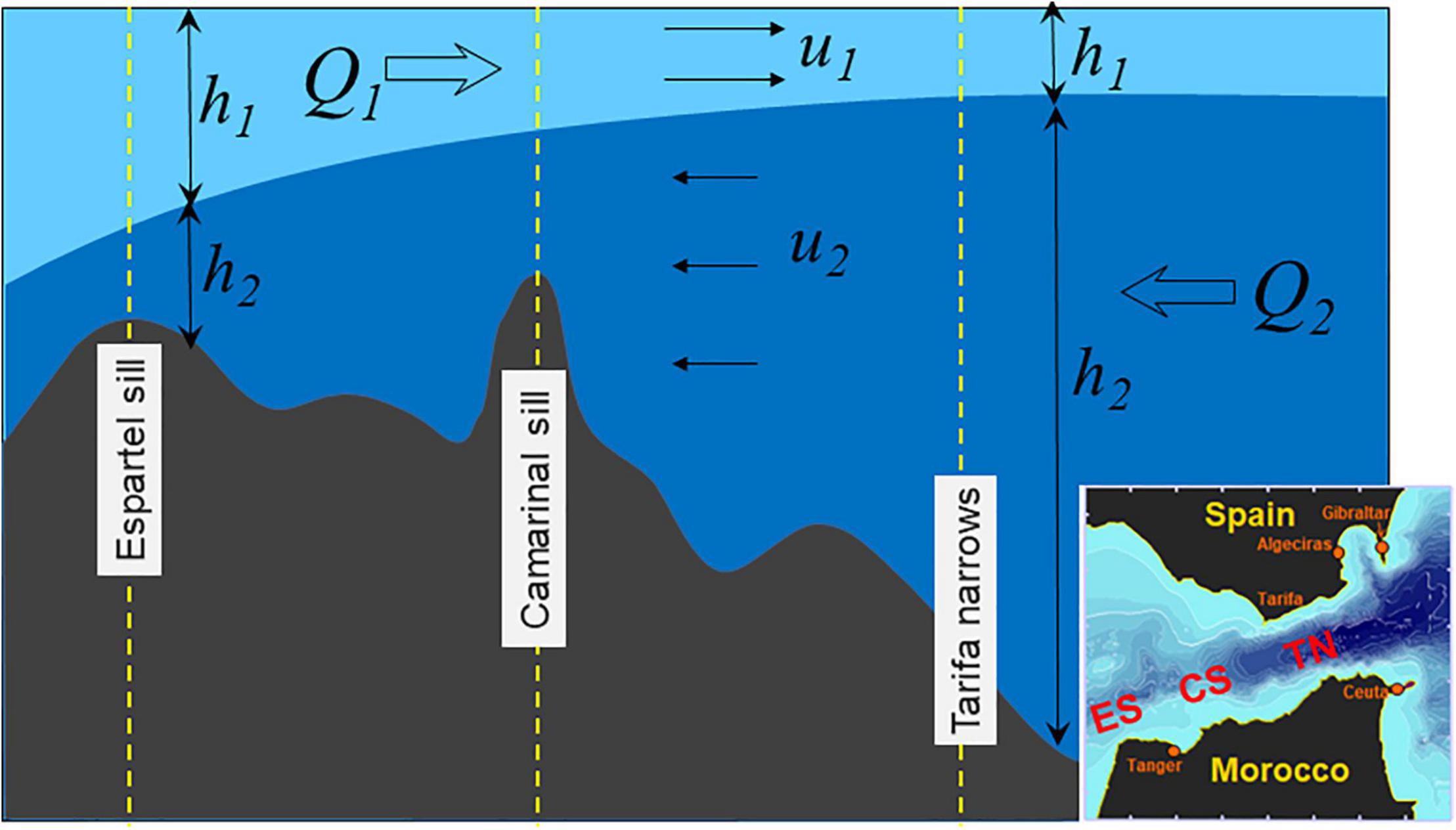
Figure 2. Sketch of the two-layer exchange in the Strait of Gibraltar. Subscripts 1 and 2 stand for variables in the upper and lower layers, whose densities are ρ₁ and ρ₂, respectively. In a steady state, Q_i’s are constant but u_i and h_i are not. The three notable topographic sections, Espartel and Camarinal sills and Tarifa narrows, have been indicated in both, the sketch and the inset map. Camarinal sill and Tarifa narrows are the candidate critical sections for steady exchange. In case of time-dependent flow (tides) Espartel sill and Tarifa narrows are much more likely candidates for critical sections (see text).

If the flows are hydraulically controlled at two critical sections connected by a region of sub-critical flow, then the exchange is maximal (Armi and Farmer, 1987). The condition G=1 is usually achieved in notable topographic sections, generally the narrowest and the shallowest. For steady exchange, the SoG fulfills these requirements at Tarifa Narrows and at the main sill of Camarinal (narrowest and shallowest sections, respectively, Figure 1) and, therefore, it is candidate to sustain maximal exchange (Farmer and Armi, 1988).

The constrain imposed by the maximal exchange together with the climatology over the basin, determine the global characteristics of the Mediterranean and link them to the flow properties at the SoG, a result of obvious interest to our study. The issue was first addressed by Bryden and Kinder (1991), who assumed a channel of triangular cross-section and a density difference brought about by salinity exclusively (Δρ = β(S₂−S₁),β the haline contraction coefficient of seawater). The salinity of the MedSea, S₂, was left as an output of the model. For a net evaporation in the basin of 0.6 m/year (equivalent to 0.04Sv), they obtained steady-state inflow Q₁ = 0.92Sv and outflow Q₂ = 0.88Sv, and ΔS = S₂−S₁≈2, close to the actual values.

At short time-scales, however, the exchange is markedly time-dependent. Tides provide a net barotropic flow strong enough to override the hydraulic control at Camarinal sill, particularly during the intensified flows of spring tides (Farmer and Armi, 1988; Sannino et al., 2004; Sánchez-Garrido et al., 2011). The loss of the control leads to the release and further radiation into the MedSea of packets of large amplitude internal waves, a well-known feature of this region (Farmer and Armi, 1988; Brandt et al., 1996; Vlasenko et al., 2009; Sánchez-Garrido et al., 2011). When this happens, the hydraulic control of Camarinal is transferred to Espartel sill, where it is in force most of the time (Sánchez-Román et al., 2009; Sannino et al., 2009). In addition, the loss of control boosts the contribution of tidally induced eddy-fluxes (positive correlations of vertical interface fluctuations and tidal currents) to the exchange (Bryden et al., 1994; Sannino et al., 2004; Vargas et al., 2006) at either critical section. Therefore, large eddy-fluxes at a control section lead to hydraulic control intermittency. Alternately, very weak eddy-fluxes (or no eddy-fluxes at all) would suggest lastingness of the control. The frequent loss of hydraulic control at Camarinal sill (Farmer and Armi, 1988; García Lafuente et al., 2000, 2009; Vargas et al., 2006; Sánchez-Garrido et al., 2008, 2011) and the large associated eddy-fluxes there (up to 0.5Sv or 40% to 60% of the total exchange; Bryden et al., 1994; Sannino et al., 2004; Vargas et al., 2006) contrast with those at Espartel (∼0.04Sv or 5%; Sánchez-Román et al., 2009; Sammartino et al., 2015). This particular behavior stresses the potential of Espartel sill replacing Camarinal sill as a long-lasting hydraulic control section.

Should the critical value G = 1 be achieved in Espartel section, it would basically be done through F₂ (equation [1]), as the large width and thickness of the surface layer (Figure 1) imply very low velocity u₁. Similar reasoning applies to F₁ in Tarifa Narrows due to the large thickness of layer 2. These approximations, already suggested by Farmer and Armi (1986), may be interpreted as if Tarifa Narrows controls the inflow Q₁, which is the active layer there, while Espartel sill does the same with the outflow Q₂. It underlines the experimental benefits of monitoring the outflow in this section in order to discriminate the state of the exchange: F₂ = 1 for possible maximal exchange (F_1 in Tarifa Narrows must be inspected), and F₂ < 1 for submaximal exchange. It also emphasizes the importance of the collected data in relation to the global properties of the MedSea, particularly in case of submaximal exchange, as it is outlined next.

Buoyancy Fluxes, Water Formation and Outflow

In our simple MedSea–SoG system the other key variable is the amount of Mediterranean water (Q_M) formed due to buoyancy fluxes (B₀) to the atmosphere, which should be equal to |Q₂| in an ideal steady-state on yearly basis. In maximal exchange (G = 1), |Q₂| has attained its maximum. If, eventually, Q_M > |Q₂| during a given period, the excess of formed water cannot flow out unless either the interface goes up or g′ increases (equation [1]), which requires larger density difference Δρ. The interface cannot rise because it would block partially the inflow, preventing the water balance of the basin Q₁ + Q₂ = (E−P) The excess of water has to remain in the basin contributing to increase its density (hence, Δρ) in successive years until reaching a new equilibrium. This is how the hydraulics of the SoG determines the MedSea properties. If, on the contrary, Q_M < |Q₂| the equilibrium is easily maintained as |Q₂| has no constrain for diminishing. But the exchange would change to submaximal. If the exchange was already submaximal, there is no impediment for |Q₂| to increase if Q_M > |Q₂| or to decrease if Q_M < |Q₂|, making G (F_2 in the previous approximation) increase or decrease accordingly. As pointed out by Garrett et al. (1990), it is only if the exchange is submaximal that changes occurring in the MedSea can bring about a non-lagged footprint in the outflow at the SoG (i.e., at Espartel section). If it were maximal, such changes would be only reflected in Q₂ after several years (Garrett et al., 1990).

The formed water Q_M is proportional to the buoyancy flux B₀, given by Gill (1982)

$$B_0=g\left[-\frac{\mathrm{\alpha }}{c_p}{Q}_{net}+{\mathrm{\rho }}_0\mathrm{\beta }S\left(E-P\right)\right](2)$$

where g is gravity acceleration, α and β the thermal expansion and haline contraction coefficients of seawater, c_p its heat capacity, and ρ₀ and S a reference density and surface salinity, respectively (g = 9.81ms^–2, α = 2.6⋅10^–4K^–1, β = 7.44⋅10^–4, c_p = 3984JKg^–1K^–1, ρ₀ = 1028kgm^–3 and S = 37 in this study). Q_net is the net heat flux into the sea (Wm^–2, positive downwards), and (E-P) is the net evaporation which includes river run-off (ms^–1, positive upwards). They give the buoyancy flux B_0 in kgm^–1s^–3 (Nm^–2s^–1). Negative heat flux (cooling) and positive net evaporation cause positive buoyancy flux to the atmosphere.

A crude estimation of the amount of water of density ρ₂ that could be formed from water of density ρ₁ under a constant and homogeneous buoyancy flux B₀ acting on a basin of area A_MED (say, the MedSea) would be

$$Q_M=\frac{B_0{A}_{MED}}{g\left({\mathrm{\rho }}_2-{\mathrm{\rho }}_1\right)}(3)$$

(for Q_net≈−3Wm^–2 and (E-P)≈0.7 m/year (=2.22⋅10^–8ms^–1), representative values of the Mediterranean basin, B₀≈8⋅10^–6Nm^–2s^–1 from equation [2], which gives the realistic value of Q_M≈1.03Sv in equation [3] with A_MED = 2.5⋅10¹²m² and Δρ≈2kgm^–3). Obviously, the actual processes of deep water formation are much more complex (pioneer paper by MEDOC Group (1970), or Houpert et al. (2016) for a recent comprehensive study). The simplicity of equation [3], however, provides a linear relationship for the expected dependence of Q_M on B₀. The simple two-layer model summarized above links Q_M and Q₂, thus extending this relationship to the outflow and the buoyancy flux, and is a well-suited first approximation for the discussion of the results presented in this study. The model, however, is a steady-state model that could be possibly extended to very slowly (long-term) varying conditions such as trends, but not to short-term scales. Therefore, the present study focuses on these long-term changes or trends.

A Short Description of the Data Sets

Currentmeter and Temperature/Salinity Data

The monitoring station at Espartel sill is located at 35°51.71′N and 5°58.22′W (Figure 1) at ∼360 m depth. The instrumented mooring line is equipped with an up-looking Acoustic Doppler Current Profiler (ADCP RDI Workhorse Long Ranger 75 kHz), embedded in a 1.5 m wide buoy deployed at ∼17 m above the seafloor, a Conductivity-Temperature sensor (CT, Seabird SBE37-SMP) and a single point current meter (Nortek Aquadopp DW), both clamped approximately 3 m below. Sampling interval for all instruments has been set to 30 min. The station was first deployed in October 2004, and has been working since, with a large gap in 2011-12 due to a line loss, and few shorter gaps due to different technical issues. The dataset used in this study covers the period from October 2004 to February 2020.

The accurate calibration of CT probes is critical because the instrumental drift of the sensors (O(10^–3)°Cyr^–1 for temperature; O(10^–3)yr^–1 for salinity) is comparable to the trends of the Mediterranean water masses characteristics reported in the literature (see Vargas-Yañez et al., 2017, for instance). CT data in this study come from a bunch of 6 different instruments, all which have been regularly calibrated throughout the probe life every one or two years. Details about ADCP datasets are presented in Supplementary Appendix A, which includes a short history of the station and other relevant issues.

Biogeochemical Data

After the gap, in year 2012, autonomous sensors for continuous recording of pH (at total scale and reference temperature of 25°C) and CO₂ partial pressure (pCO₂, μatm) (SAMI-pH and SAMI-pCO₂, Sunburst Sensors, LLC.) were incorporated to the monitoring line and placed at the same depth as the CT probe. Unfortunately, the instruments were lost in year 2017 after an accident underwent by the mooring line and they have not been replaced until very recently. It reduces the pH data availability from August 2012 to March 2017, and to a shorter period in the case of pCO₂ data. The sampling interval was initially set to 60 min, but a battery run off happened in summer 2013 (which caused a six-month data gap) advised changing the interval to 120min to extend the battery life.

According to manufacturer, precision and accuracy of measurements were ∼0.001 and ± 0.003 units for pH and ∼ 1 μatm and ± 3 μatm for pCO₂, approximately. Repeated measurements conducted in the laboratory with the probes submersed in aged seawater and high CO₂ seawater to validate these specifications provided values of ∼0.003 and ± 0.005 units for pH and ∼3 μatm and ± 5 μatm for pCO₂. SAMI-devices were nonetheless, regularly checked upon periodic servicing of the line on board and pH data obtained by the spectrophotometric technique (Clayton and Byrne, 1993) in samples collected in oceanographic cruises carried out in the area were used to validate the series and identify possible drifts and drops of the autonomous sensors (see section “Other Biogeochemical Properties”). Thus, samples at the mooring site were taken within the Mediterranean outflow in August 2012 (4), May 2013 (4), November 2014 (2), June 2015 (5), and March 2017 (9) under the frame of the Gibraltar Fixed Time Series monitoring program (GIFT, Flecha et al., 2019). Samples were taken directly from Niskin bottles in 10 cm path-length optical glass cells and submitted to a Shimadzu UV-2401PC spectrophotometer containing a 25°C-thermostated cells holder after addition of m-cresol purple as indicator. Precision and accuracy of these discrete and independent pH_T25 measurements were determined from measurements of certified reference material (CRM batches #97 and #136 provided by Prof. Andrew Dickson, Scripps Institution of Oceanography, La Jolla, CA, United States) and were equivalent to ± 0.0048 and ± 0.0047 units for pH_T25.

Other Data

Data of mass and heat fluxes to the atmosphere from the fifth generation of ECMWF atmospheric reanalysis of the global climate (ERA5, Hersbach et al., 2020), distributed by the Copernicus Climate Change Service (C3S), have been retrieved in order to estimate buoyancy fluxes in the Mediterranean basin.

Water Properties of the Outflow at the Monitoring Station

Temperature, Salinity, Density

Figure 3 displays the potential temperature θ registered at ∼14 m above the seafloor in the monitoring site. This short distance implies that the instrument is sampling the densest (hence, coldest) water that leaves the MedSea. Temperature fluctuates noticeably at tidal timescale due to mixing (light-gray dots in Figure 3). It is not local mixing (the instrument is far enough from the interface for local mixing to reach its depth) but advection of waters mixed upstream in the Tangier basin (Figure 1), where intense mixing happens (Wesson and Gregg, 1994). Conventional numerical filtering is not advisable to remove these fluctuations because the low-passed series smooths out the footprint of the coldest samples, which are particularly relevant since they inform about the deepest waters that are leaving the MedSea. A possibility of removing tidal fluctuations without losing this information is to extract the coldest sample in each semi-diurnal tidal cycle and decimate the series to a sample per cycle (García Lafuente et al., 2007; Naranjo et al., 2012, 2017). Light-blue dots in Figure 3 show the resulting series where most semidiurnal and diurnal tidal variability has been removed.

FIGURE 3

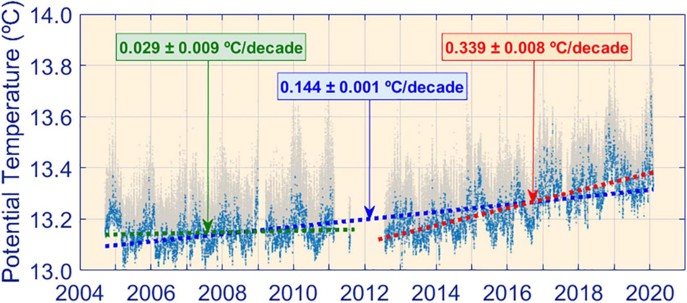
Figure 3. Potential temperature at 14m above seafloor in the monitoring station sampled every 30 min (gray dots) and series of minimum θ in each tidal cycle (light-blue dots). Dashed lines show θ trends for the whole period (blue line), from the beginning of the series to the data-gap in 2011-12 (green line), and from the gap to the end of the series (red line).

Dashed-blue line in Figure 3 shows a clear trend of 0.144°C/decade in θ (see also Table 1). This value, however, is misleading as the trend during the first half of the record is much less (0.029°C/decade, dashed-green line), whereas it is more than double in the second half (0.339°C/decade, dashed-red line). It seems to be around year 2013 that the trend changed. And it did in an order of magnitude with regards to the before-2012 value! Although this pattern was anticipated in Naranjo et al. (2017), they could not give definitive ratification as they used a correspondingly shorter length of this time series (up to year 2015). The extended series available nowadays does confirm the existence of that trend, which is so large and unexpected that has motivated the present study.

TABLE 1

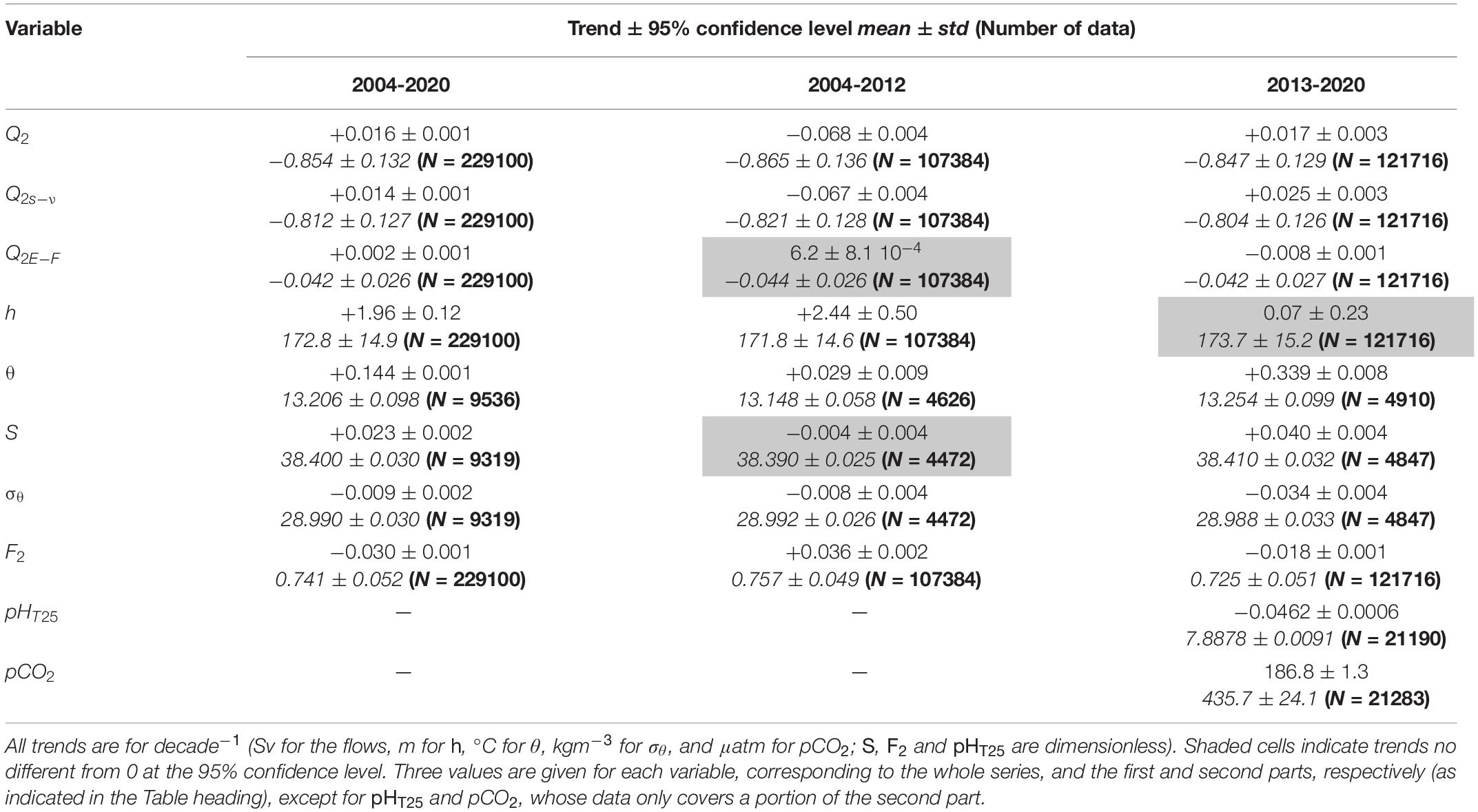
Table 1. Summary of estimated trends (with 95% confidence level), mean and std (in italics) and number of data used in each calculation (in bold in brackets) for different variables of the study: Q₂ is the total outflow, Q_2s–ν is the slowly part of it and Q_2E–F is the tidally driven contribution of the eddy-fluxes; h is the interface height, θ is the potential temperature, S the salinity, σ_θ the density anomaly, F₂ the lower layer Froude number, pH_T25 the seawater pH and pCO₂ the CO₂ partial pressure.

Similar analysis has also been carried out for salinity, S. Only salinities corresponding to the samples of minimum θ have been selected in order to use the same subset of data for both variables. The analysis yields a positive trend of 0.023 decade^–1 for the whole series (Table 1), which increases to 0.040 decade^–1 in the second part of the series after the year 2012 gap. Before 2012, the trend does not differ from 0 within the 95% confidence level (Table 1). Because of the opposite effects of temperature and salinity, the density trend depends on the relative weight of θ and S trends. In this case, the former prevails and the trend of density anomaly σ_θ is negative: −0.009 kgm^–3/decade for the whole series (Table 1). It changes markedly to −0.034 kgm^–3/decade in the second part of the series as a consequence of the sharp increase of θ during the same period.

These results are illustrated in the θ-S diagrams of Figure 4. The available data have been grouped together by years. As the monitoring station was first deployed in October 2004, years have been defined from October 1 to September 30 of the following year: year 2005 goes from October 1, 2004 to September 30, 2005 and so on. Light-blue dots in the top-left panel show the data sampled at Δt = 30min during the first three years (2005, 2006, 2007, see legend), and red dots do the same for the last three years (2018, 2019, 2020). The increase of potential temperature of the water flowing past the station is palpable. The rise of salinity and the diminution of density are less obvious but still detectable.

FIGURE 4

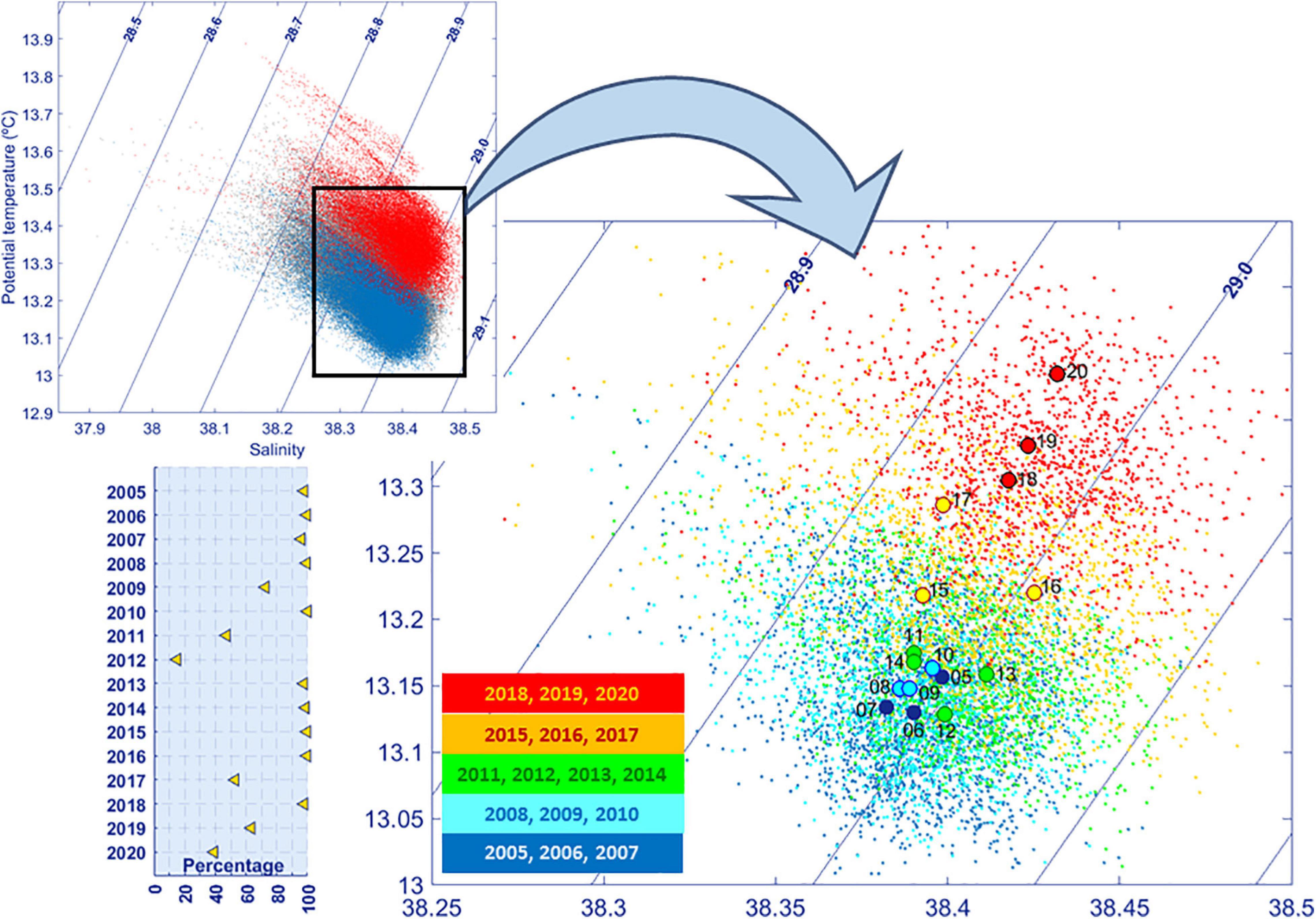
Figure 4. θ−S diagram of the data recorded by the station. Top-left diagram shows the data sampled every 30 min during the first (blue dots) and last (red dots) three years, respectively (see text for definition of “year”). Black rectangle indicates the portion of the diagram enlarged in the right panel. Dots in this diagram correspond to the samples of minimum θ extracted from the whole series. They have been colored by years, according to the code in the legend. Large dots are the mean value of a given year, labelled next to them, and follow the same color code. The percentage of data available each year is indicated in the bottom-left plot: 100% correspond to 17520 30 min-data or 705 minimum-θ-data per year.

Right panel shows the samples of minimum θ and their yearly mean (large dots). The lack of data in some years can bias the mean, as it could be the case of year 2012 with a low percentage of data (bottom-left plot), although, curiously, it remains close to the neighbor years. The distribution of large dots clearly suggests two different periods, a pattern that would still stand even if some means are biased: a first one from 2005 to 2014 when years group close together around θ = 13.15°C, S = 38.4, and a second period of continuous and marked rise of mean θ and also of S to a lesser extent, with the exception of year 2016. The partition agrees with the previous one found in the analysis of trends.

Other Biogeochemical Properties

Figure 5A shows the pH time series in total scale at a reference temperature of T = 25°C (pH_T25) measured at the monitoring station. No data during the first part of the series are available, as the biogeochemical sensors were only deployed in summer 2012. Therefore, they illustrate the temporal evolution of this variable in the Mediterranean outflow until 2017.

FIGURE 5

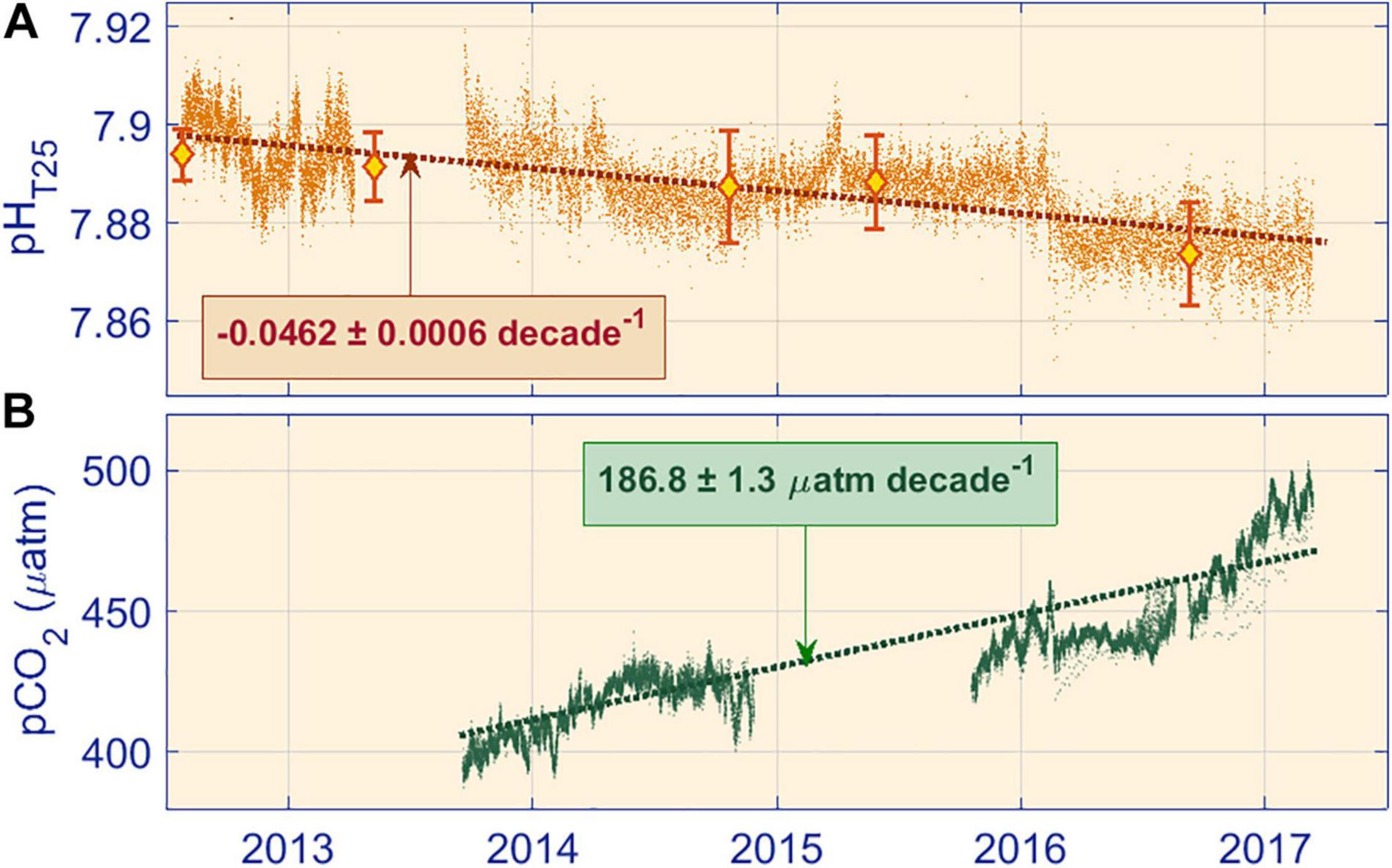
Figure 5. (A) Time evolution of the SAMI-pH data and the estimated linear trend (dashed line) from August 2012 to March 2017. (B) Same as (A), but for pCO₂ data. Red diamonds and associated bars in panel (A) are the mean and std of the discrete pH_T25 values obtained directly from seawater samples through the spectrophotometric technique.

These series have been contrasted against the discrete spectrophotometric pH values deduced from the seawater samples collected in the outflow layer during the five cruises that overlapped the monitoring period. The resulting pH_T25 values, which come from independent samples, are shown in Figure 5A in red symbols, and agree with the overall trend of the series quite satisfactorily.

During the four-and-half-year period, pH_T25 data ranged between a maximum of 7.9193 measured in October 2013 to a minimum of 7.8520 in January 2017 and exhibits the expected trend to diminish in the present scenario of ocean acidification, a trend also confirmed by the values obtained through spectrophotometry (red diamonds in Figure 5A). The decrease is not steady but step-like, the most obvious jump occurring in early 2016. Overall, the series shows a remarkable negative trend of −0.0462 ± 0.0006 decade^–1, significant at the 95% confidence level.

Figure 5B shows complementary in situ pCO₂ data from the SAMI sensor, which exhibits a trend inversely and significantly correlated to that of pH_T25 (not shown). During the period of available data, the pCO₂ in the outflow at the depth of the monitoring station showed a remarkable rise of 186.8 ± 1.3 μatm decade^–1. Nevertheless, and in concordance with the pH_T25 series, pCO₂ evolution did not exhibit a smooth increase but a more evident rise from early 2016.

The Interface Between Atlantic and Mediterranean Waters

The first step to estimate the Mediterranean outflow is the computation of the height of the interface between Atlantic and Mediterranean waters, which implicitly requires a definition of interface. Much has been written about this issue and different solutions have been proposed (Bryden et al., 1994; García Lafuente et al., 2000, 2011, 2019; Tsimplis and Bryden, 2000; Sánchez-Román et al., 2009, 2012; Naranjo et al., 2014; Sammartino et al., 2015). The depth of null velocity, the obvious definition in a two-way steady exchange, is not applicable due to tidally driven reversal of the flows, which makes both layers to flow in the same direction during a portion of the tidal cycle and prevents zero-velocity from being achieved. Selecting a material surface is another possibility. Salinity is the best candidate and specific isohalines have been proposed and used to this aim (Bryden et al., 1994; García Lafuente et al., 2000, 2013, 2019). It requires time series of S profiles throughout the water column. If they are not available, which is the case in this study, the procedure is not affordable. A third possibility is to link the interface position with the depth of maximum vertical shear of horizontal velocity (Tsimplis and Bryden, 2000; Sánchez-Román et al., 2009, 2012; Naranjo et al., 2014; Sammartino et al., 2015). The technique is well suited to the available series of ADCP velocity profiles and has been adopted here. The detailed description of the procedure can be seen in Sammartino et al. (2015) and has been followed to the letter in this work.

Figure 6B shows the time evolution of the interface height h₂ at the monitoring station, whose mean value is 172.8 m from the seafloor (Table 1). A marked subinertial variability stands out (the substantially larger tidal oscillations have been filtered out) overlapping an unclear, but still recognizable, seasonal cycle with the interface higher in spring and deeper in late summer-autumn. A comprehensive description of these issues can be seen in Sammartino et al. (2015) and are not addressed here. For the purpose of this work, the result of interest is the trend of the interface to become shallower at a rate of 1.96 m/decade. Following the splitting of the whole series in two parts suggested by θ (Figure 3), the same differentiation has been accomplished with this series. Table 1 indicates that most of the interface elevation took place in the first part before the data gap of year 2012, whereas the trend is not significantly different from 0 at the 95% confidence level during the second one.

FIGURE 6

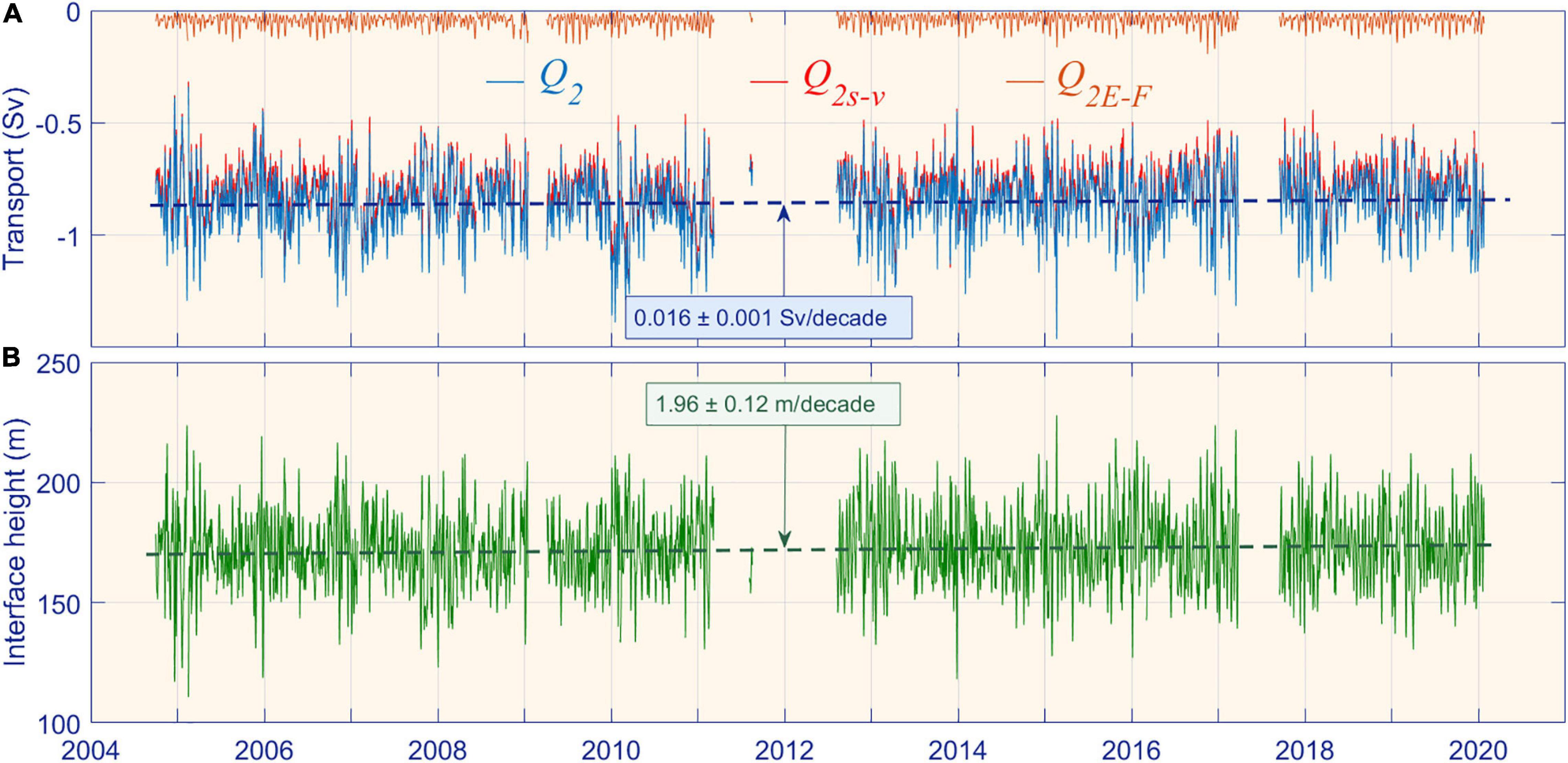
Figure 6. (A) Total outflow Q₂ at Espartel section computed from the available velocity profiles (blue line), and the slowly varying Q_2s–ν (red line) and eddy-fluxes Q_2E–F (sienna line) contributions (see text for details). Deep-blue dashed line is the linear trend in the whole period. (B) Interface height h₂ at the position of the monitoring station and its linear trend (dashed-green line). All series have been filtered to remove tidal variability so that the marked fluctuations in both panels reflect subinertial and seasonal variability.

The Estimated Outflow

The outflow Q₂ has been also calculated following the procedure in Sammartino et al. (2015) after revising the lower part of the vertical profiles of horizontal velocity. The revision has been motivated by the availability of near-bottom velocity data collected by a new instrument incorporated into the monitoring station since September 2016. The data offer an ameliorated description of the bottom boundary layer and compel to modify the vertical profile of velocities within a few tens of meters above the seafloor with regards to the profile used in Sammartino et al. (2015). A detailed explanation of how it has been recalculated in light of these new data is presented in Supplementary Appendix A.

The low-passed (subinertial) outflow Q_2 computed with the new profiles (Figure 6A, blue line) differ only slightly from the one computed using Sammartino et al. (2015)’s velocity profiles. Its mean value (2004 to 2020) is -0.85 ± 0.13 Sv (standard deviation), whereas it is −0.82 ± 0.16 Sv if Sammartino et al. (2015)’s profiles were used instead. The ameliorated estimation gives a 3.7% greater and, also, less fluctuating outflow. Of interest is the positive trend identified in the whole series of Q₂ (Figure 6A, dashed-blue line, Table 1), estimated in +0.016 Sv/decade (Table 1). Since Q₂ is negative, this trend diminishes the outflow. Care must be taken, however, because the trend was negative before the gap of year 2012 (Table 1), meaning that Q_2 was increasing during the first part, to reverse the tendency in the second one.

Red line in Figure 6A displays the slowly varying part of the outflow (Q_2s–ν), which results from filtering out tidal fluctuations from the horizontal velocity and interface motions, and computing the transport with the low-passed series. The result differs from the total outflow (blue line) because of the already mentioned eddy-fluxes (Q_2E–F; see Vargas et al., 2006, for details about Q_2s–ν and Q_2E–F computations), which hardly contribute by ∼5% to the outflow (sienna line in Figure 6A, see Table 1) in agreement with Sánchez-Román et al. (2012) and Sammartino et al. (2015). Both terms exhibit positive trends for the whole series (Table 1), the trend of Q_2s–ν being comparable to the one of Q₂, whereas the trend of Q_2E–F is much smaller. During the second part the sign of both trends is different (Table 1), a fact that will be discussed later.

Interpretation of Results

The Froude Number at Espartel Section

The Froude number at Espartel has been computed in order to assess the hydraulic state of the exchange. The lack of information in the upper layer only allows for the estimation of F₂ in equation [1]. Notwithstanding and according to the arguments given in Section “The Hydraulically-Controlled Exchange Model”, F₂≈G is a reasonable approximation and, therefore, F₂ is a good indicator of that state. It can be evaluated in terms of Q₂ (instead of u₂) and the interface height h₂ as (see Supplementary Appendix B and Supplementary Figure B1 for details)

$$F_2=\frac{\left|Q_2\right|{\left(W_b+c{h}_2\right)}^{1\mathrm{/}2}}{{\left(W_b{h}_2+0.5c{h}_2^2\right)}^{3\mathrm{/}2}{g}^{\prime 1\mathrm{/}2}}(4)$$

for a realistic trapezoidal cross section of bases W_b(=2100m) at the sea bottom and W₀(=7000m) at the mean height of the interface H₀(=173m). Dimensionless constant c is defined as c = (W₀−W_B)/H₀ = 28.32. Figure 7 displays the time series of F_2 computed from the series of Q₂ and h₂ presented in Figure 6.

FIGURE 7

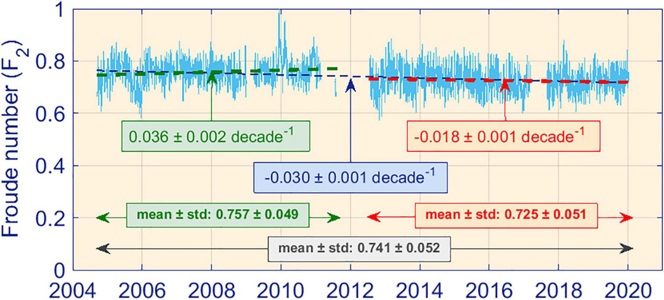
Figure 7. Time evolution of the lower layer Froude number (F₂) computed according to equation [4]. Dashed blue line is the linear trend for the whole series and dashed green and red lines show the trends before and after the gap of year 2012, respectively. All numerical values, including 95% confidence levels, are indicated inside the text-boxes with the same color code. Mean and standard deviation for the whole series, and for the first and second parts are also indicated.

Except for an isolated event by the end of year 2009, F₂ does not reach the critical value of 1. Including F₁ in the estimation of G in equation [1] does not change the result because F₁ hardly reaches 0.1 due to the low vertically averaged velocity u₁ in this section. Despite being close, Espartel does not meet the condition of critical section and, therefore, the exchange is not maximal, but submaximal. Greater exchanged flows are possible.

Figure 7 indicates a decreasing trend of F₂, which could have been anticipated from the tendencies of Q₂ to diminish in magnitude and h₂ to increase (Figure 6), as both them act in the same direction to diminish F₂ (equation [4]). The simultaneity of such trends in Q₂ and h₂ are counterintuitive: the higher the interface, the larger the cross-area for the Mediterranean water to flow out. The expected result would be an increased outflow and not a diminution. The explanation of the paradox is in Table 1. The rise of the interface took place during the first part of the series previous to the data-gap, when Q₂ had negative trend that increased the magnitude of the outflow. It is the intuitive physical behavior, which leads to a positive trend of F₂ in this first part (Table 1). Thus, F₂ increased driven by the augmented outflow, which approached maximal exchange conditions that, in the end, did not attain. The interface had no significant trend during the second part whereas the one of Q₂ changed sign (Table 1), reducing progressively the outflow and, therefore, F₂.

Buoyancy Fluxes and Water Formation

Figure 8A shows the yearly value of B₀ averaged during winter months from 2004 to 2020, using the outputs of ERA reanalysis. There is a marked interannual variability with years of strong buoyancy flux, which supposedly correspond to years of large volume of newly formed deep water. It is the case of year 2005 (Schroeder et al., 2008) or years 2009, 2010, 2012 (Houpert et al., 2016) with regards to the WMDW in the western MedSea. But there also exists years of weak buoyancy flux such as 2008 or 2011, when no WMDW was reported to have been formed (Houpert et al., 2016).

FIGURE 8

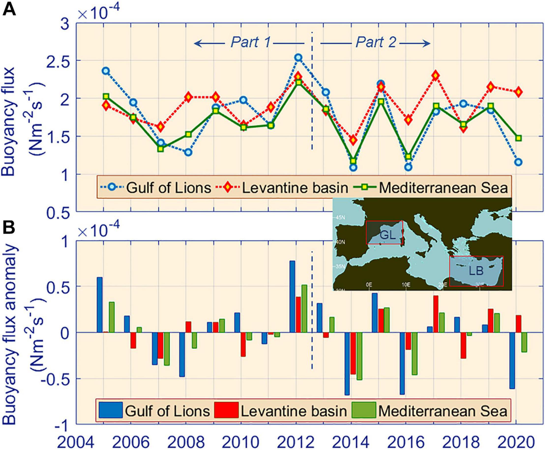
Figure 8. (A) Time-averaged buoyancy flux B₀ during winter months (December, January and February) from 2004 to 2020 (sixteen data, starting in December 2004 and ending in February 2020). The fluxes have been spatially averaged for three regions, Gulf of Lions (GL in the inset map), Levantine basin (LB in the map) and the whole MedSea, as indicated in the legend. (B) Buoyancy flux anomaly of the data showed in panel (A) referred to the 2004-2020 mean. Vertical dashed line separates parts 1 and 2.

In the Gulf of Lions, buoyancy flux of three out of the seven last years, namely 2014, 2016 and 2020, had the largest negative anomaly of the whole series (Figure 8B). Except for year 2020, the same applies to the whole basin (green bars). They showed minima well below the mean, which makes the second half of the period be negatively anomalous in both, the Gulf of Lions and the whole basin. These results agree with Margirier et al. (2020), who indicate the absence of intense deep convection in the Gulf of Lions between 2014 and 2017 (their study ends in year 2018). Interestingly, this period coincides with the second part of the oceanographic observations, when the strong trend of θ was detected in the monitoring station. The coincidence encourages a similar partition of the B₀ series and estimating the trends before and after year 2013 separately.

Table 2 shows the results of such analysis. In addition to the three-winter-month averages presented in Figure 8 (DJF, Winter3 block in Table 2), two other averages have been considered: five-winter-month (NDJFM, Winter5 block) and all year round (Annual block). Trends are given in Nm^–2s^–1decade^–1 and the cells in Table 2 have been tagged according to the sign of the estimated trend. They are no-significant at the 95% confidence level, which is not surprising considering the reduced number of data-points in the fits. There is, however, a remarkable pattern in the Table: all trends during the period 2013-2020 are negative except for the positive one found in the Levantine basin in block Winter3 (although it is the less positive of the three trends in Winter3 block). Moreover, most trends in the period 2005-2012 are positive (Gulf of Lions and MedSea in block Winter5 are the exceptions). All in all, the conclusion that during the first part of the series the trend of the buoyancy was positive and changed to negative during the second part is reasonably supported. Equation [3] would indicate the same signs in the trends of Q_M. Within the framework of the two-layer SoG-MedSea model with balance between water production and export, during the first part Q₂ should increase (negative trend, as it is a negative quantity) and decrease during the second part (positive trend), which is what Table 1 reflects.

TABLE 2

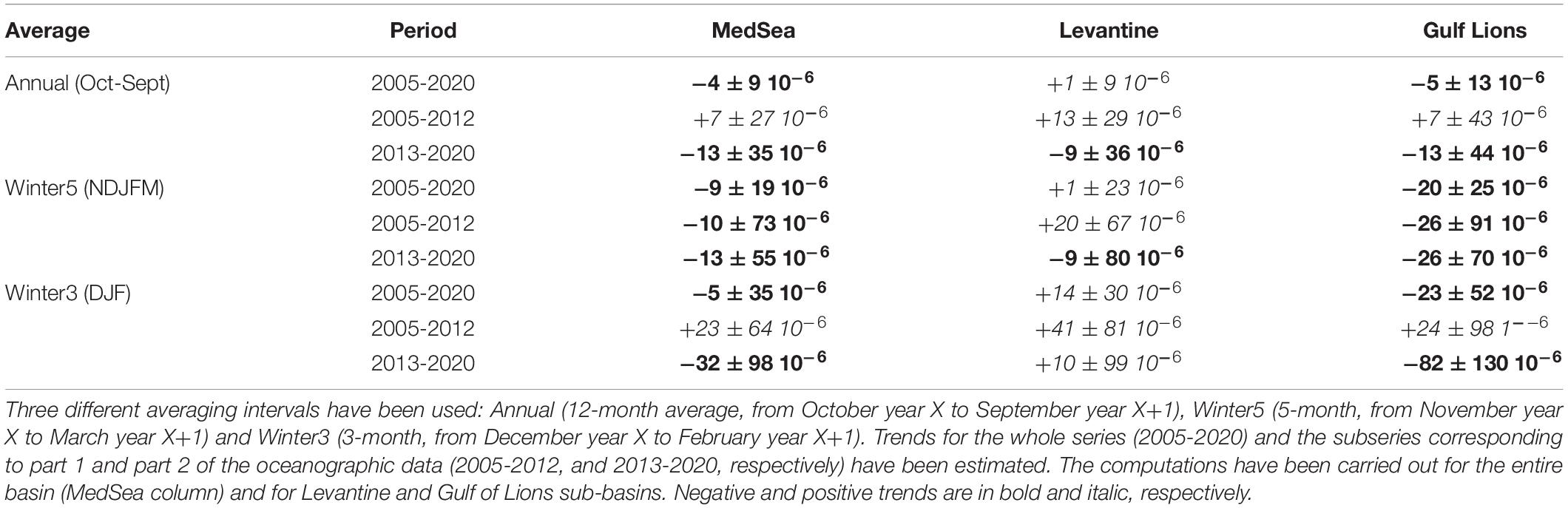
Table 2. Estimated trends of averaged buoyancy flux (Nm^–2s^–1/decade) during the period of available data in the monitoring station with the 95% confidence interval.

Fraction Composition of the Outflow

The time evolution of the properties of the water flowing pass the monitoring station may be the result of changes in the proportion of the Mediterranean waters in the outflow, or a concomitant evolution of the properties of each of the Mediterranean waters that form the outflow, or both. We focus on the WMDW and LIW, which are the main bulk of the outflow at the monitoring station, the rest being a very small fraction of Atlantic water, mainly North Atlantic Central Water (NACW) entrained by the Mediterranean flow a short distance upstream in the Tangier Basin (García Lafuente et al., 2007, García Lafuente et al., 2011).

An estimation of the fraction of the different water masses in the outflow has been carried out following García Lafuente et al. (2007). The triplet of points used by these authors was [12.8°C, 38.45], [13.22°C, 38.56] and [15°C, 36.2], representing WMDW, LIW and NACW, respectively. The water masses characteristics change from place to place and with time, and there are no unique values to represent them. A requirement for the fraction analysis to be feasible is that the θ-S points of the water samples to be decomposed lay inside the triangle defined by the triplet of reference to avoid fractions greater than 1 or less than 0, which have no meaning. The selection of the triplet is a trade-off between fulfilling this requirement and maintaining values as representative of the implied water masses as possible. The points used in García Lafuente et al. (2007) do not fulfill the first condition with the present series (left panel of Figure 9) because data of the available series at that time were grouped closer to WMDW-type (cooler, see Figure 4). A new triplet has been therefore chosen to enclose all data: [12.9°C, 38.45], [13.42°C, 38.57] and [16°C, 36.2] for WMDW, LIW and AW, respectively (Figure 9).

FIGURE 9

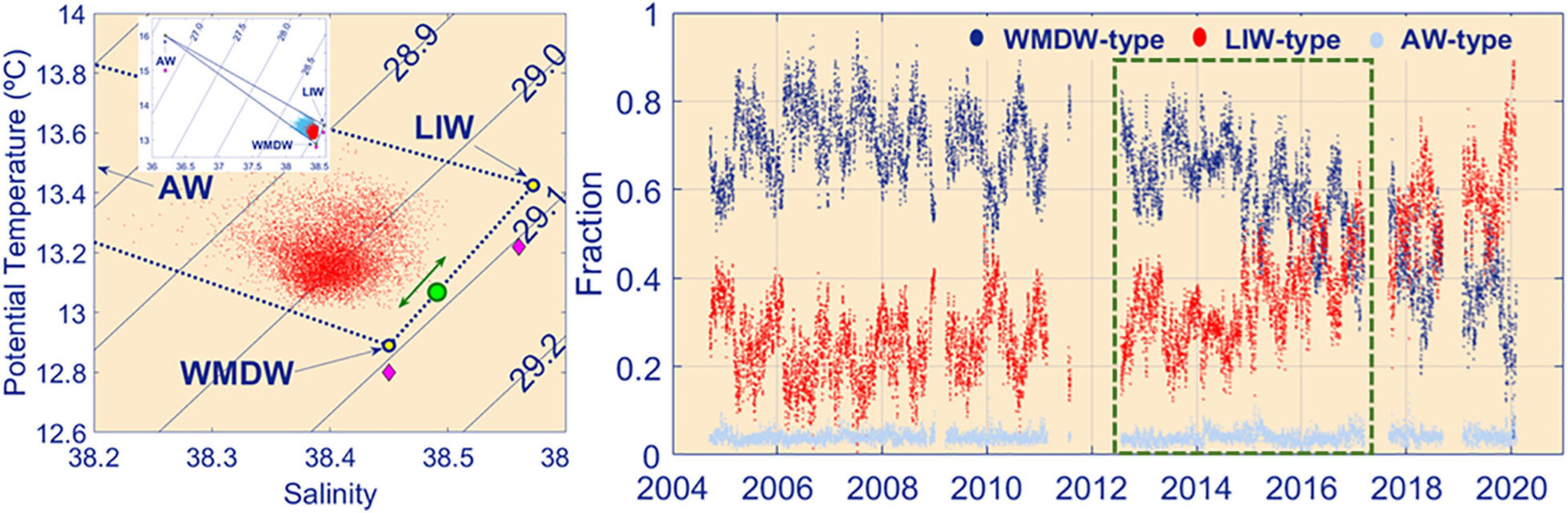
Figure 9. Left panel: θ−S diagram of the θ-minimum samples. Circles indicate the triplet of reference used for the fraction decomposition. The inset is the θ-S diagram for all (light blue dots) and θ-minimum (red dots) samples, included to show that all samples lay inside the triangle defined by the triplet. Magenta diamonds are the points used in García Lafuente et al. (2007). Green circle and the arrow represent a hypothetical evolution of WMDW-type along the line joining the initial WMDW and LIW that would change the initial triplet (see text for more explanations). Right panel: time evolution of the fraction of the different waters using the triplet initially defined. Dashed green rectangle embraces the period of available biogeochemical data.

The first hypothesis that the time evolution of water characteristics stems from changes in the fractions of each contributor implicitly assumes that the θ-S characteristics of the triplet remain unchanged. Right panel of Figure 9 shows a sudden increase of LIW-type fraction from year 2015 onwards, along with a corresponding diminution of the WMDW. The fraction of AW was kept essentially unaffected. LIW would become the main contributor in the mixing after year 2017, replacing the prevailing role of WMDW before this year.

The second hypothesis is that the time evolution of water properties in the monitoring station was the result of a concomitant change of properties of the water masses participating in the outflow instead of variations in the fractions. To keep water samples after year 2015 with, approximately, the same fractions as before 2015, the WMDW-type characteristics should evolve to saltier and warmer, as sketched by the green dot in Figure 9. By the end of the series (February 2020), its new θ-S values should be [13.1°C, 38.50] assuming a simple evolution along the dotted line joining the initial values assigned to WMDW and LIW. Right panel suggests that the starting time of the change would have been the beginning of year 2015, which would imply trends in WMDW of ∼0.4°C/decade and ∼0.1 decade^–1 for θ and S, respectively, during the last five years.

There are no numerical values in the literature for such a recent period to check with, but these trends in WMDW are clearly unrealistic. For instance, Vargas-Yañez et al. (2017) report 0.03°C/decade and 0.02 decade^–1 in the 600m-to-bottom layer in the Alboran Sea during 1943-2015; Houpert et al. (2016) indicate annual changes of 0.0032 ± 0.0005°C and 0.0033 ± 0.0002 for θ and S during the period 2009-2013 in the 600-2300 m layer in the Gulf of Lions (equivalent to trends of 0.032 ± 0.005°C/decade and 0.033 ± 0.002decade^–1). They are one order of magnitude less than the rate necessary to validate the second hypothesis, which therefore should be discarded. Certainly, the trend could be partially due to the warming and salinification of LIW instead of WMDW. To this regard, a noticeable warming of LIW in the Gulf of Lions from 2007 to 2018 has been recently reported (Margirier et al., 2020). Even so, a consistent diminution of the proportion of WMDW in the Mediterranean outflow at the depth of the monitoring station is still necessary for that warming to manifest itself in the form of the observed trend in the Mediterranean outflow. Thus, the approach followed in this work is that the recent θ-S changes in the monitoring station (Figure 3) have been mainly caused by the progressive increase of LIW fraction in the outflow and the corresponding diminution of WMDW from around year 2013 onwards.

Estimates of PH and PCO₂ in the Outflow Water Masses

Figure 5 illustrates a remarkable acidification of the Mediterranean outflow at the monitoring station, particularly from 2016 onwards. As in the case of θ discussed above, the observed pH_T25 and pCO₂ trends could be the result of similar trends in the LIW and WMDW, the main components of the outflow, the change with time of the fractions of each water mass in the outflow, or both. In order to gain insights on the origin of this issue, the fraction analysis performed above (Figure 9, dashed-green box) was combined with the multi-linear regression model developed by Flecha et al. (2015) to obtain the individual pH_T25 and pCO₂ values characterizing the LIW and the WMDW separately. This procedure has been applied successfully to discriminate between the components of the outflow and to estimate the values of oceanographic properties in each water body separately (Flecha et al., 2012, 2015, 2019). Figure 10 displays the time evolution of the pH_T25 and pCO₂ assigned to each water mass in the outflow from 2012 to 2017.

FIGURE 10

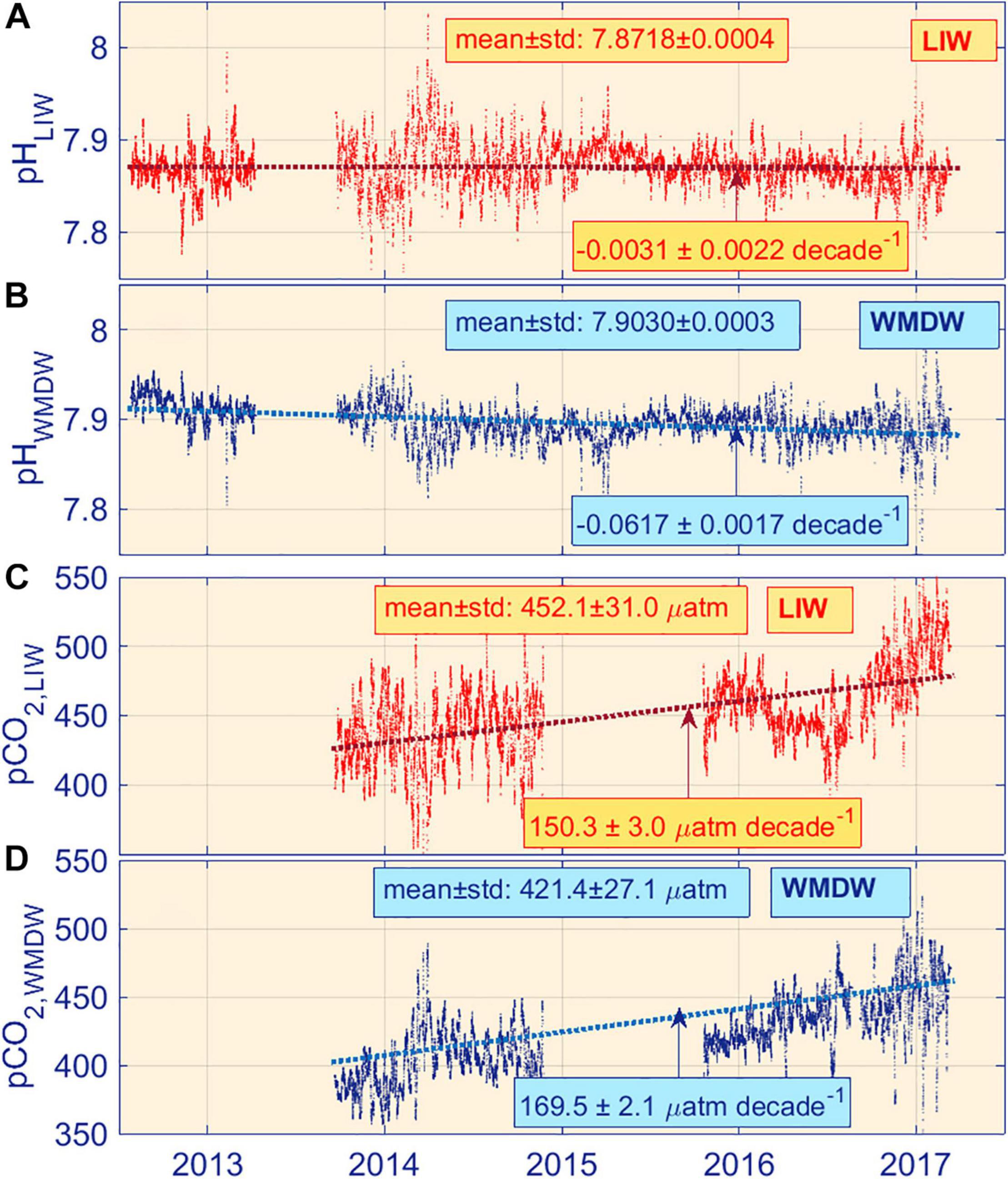
Figure 10. (A) and (B). Time series of pH_T25 assigned to LIW and WMDW, respectively, applying the water masses fraction analysis specified in Section “Fraction Composition of the Outflow.” (C) and (D) Idem for pCO₂.

The analysis provides time-averages of 7.8718 ± 0.0004 and 7.9030 ± 0.0003 for pH_T25 of the LIW and WDMW, respectively (Figure 10), values that are slightly lower than those reported by Flecha et al. (2015) who used a shorter time series spanning from 2012 to 2015. The difference can be interpreted as a gradual acidification attributed to the increase in CO₂ content in the Mediterranean waters. In fact, during the last portion of the available pH data (June 2015 to March 2017), the time-averages of the pH_T25 series dropped to 7.8654 ± 0.0005 in the case of LIW and 7.8978 ± 0.0004 in WMDW, which were accompanied by a rise of pCO₂ (Figures 10C,D).

The four-and-half-year time series in this study also revealed a striking and sudden decrease of pH_T25 by the beginning of year 2016 in the outflow. It occurred concomitantly with a progressive rise in pCO₂ (Figure 5), the trends in both properties remaining relatively stable from then onwards. Signatures of the pH_T25 decrease and pCO₂ rise can be indeed detected in the LIW and WMDW separately (Figure 10) and therefore, it is plausible to assume that both water masses are contributing to the overall patterns detected in the outflow. However, water fraction analysis reveals that the warmer LIW prevailed in the outflow from January 2016 with the corresponding decline of WMDW fraction (Figure 9, green box), a situation more evident in the spring of this year. Fractions kept increasing (LIW) and decreasing (WMDW) rather steadily from September 2016 onwards.

According to former studies that used shorter series of this SAMI pH dataset (up to 2015, Flecha et al., 2015) or discrete pH_T25 measurements (Flecha et al., 2019), LIW was invariably characterized by pH_T25 values lower than those in WMDW and relatively constant. These results agree with previous studies that report pH minima in the LIW in several Mediterranean sub-basins in relation to the rest of Mediterranean waters (Alvarez et al., 2014; Hassoun et al., 2015). Such minima have been attributed to the remineralization of organic matter during aging of the LIW. As this water flows at intermediate depths isolated from the atmosphere in its way back to the Atlantic ocean, anthropogenic carbon absorption is prevented, making its pH levels remain stable (Alvarez et al., 2014). On the contrary, deep convection and/or shelf water cascade that drive the winter formation of WMDW from the very surface in the Gulf of Lions accumulates anthropogenic carbon in the newly formed water, which favors a WMDW acidification trend (Hassoun et al., 2015; Flecha et al., 2019). Patterns of pH_T25 and pCO₂ up to 2015 in Figure 10 corroborate these findings: lower but relatively constant pH_T25 in the LIW versus higher but decreasing-over time pH_T25 in the WMDW. But Figure 10 also suggests a novel acidification trend in the LIW since 2016, which, along with the suggested prevalence of LIW fraction over that of WMDW in the observed outflow (Figure 9), would result in the pH_T25 and pCO₂ trends visible in Figure 5 during the last one year and a half of data.

Discussion and Conclusion

Despite a few vicissitudes inherent to field work in harsh environments, the monitoring station deployed at Espartel sill in the SoG in late 2004 is providing worthy information about the outflow of the Mediterranean water and its properties. The outflow in turn reflects changes in the MedSea and provides an integrated overview of what is going on in the basin. Investigating likely links between changes in the MedSea properties and the outflow is the objective of this study.

A sequence of misfortunes in the experimental work caused an important data gap around year 2012. A detailed inspection of the series of collected and derived variables suggests two distinct periods in the series, with differentiated patterns of time evolution: a first period before the gap (2004-2012) and a second one after the gap (2013-2020). The most striking result is the trend of θ, which increased markedly starting by year 2013 and kept on up to the date of writing this work. In fact, the change was so outstanding (Figure 3) that not only motivated the inspection of the other variables searching for similar patterns, but also the present study.

The total outflow Q_2 showed an overall small positive trend of +0.016Sv/decade (Table 1), which reduces its size. During the first part, however, the trend was negative, −0.068 Sv/decade (the outflow increased), and then it changed sign after the gap in the second part (Table 1). The contribution of the eddy-fluxes Q_2E–F to the total outflow deserves a little attention. In Espartel section Q_2E–F hardly reaches −0.04Sv or ∼5% (Table 1), in agreement with previous findings (Sánchez-Román et al., 2009; Sammartino et al., 2015). The percentage is very similar to the one in the eastern section of the SoG (García Lafuente et al., 2000; Baschek et al., 2001; Sannino et al., 2004). The smallness of Q_2E–F in these two sections points at a two-layer exchange hydraulically controlled at Espartel sill (instead of Camarinal) and Tarifa Narrows and the possibility of maximal exchange. Notwithstanding, the latter was not achieved (F₂≈0.74 < 1, Figure 7).

An interesting fact in this regards is the behavior of the two components of the total outflow, Q_2s–ν and Q_2E–F. In the first part of the series, the trend of Q₂ originated in Q_2s–ν, Q_2E–F having no contribution (Table 1). In the second part, however, the positive trend of Q_2s–ν was noticeably higher than the trend of Q₂ and a negative trend of Q_2E–F was necessary to conciliate the mismatch. As Q_2E–F is negative, eddy-fluxes increased in magnitude, whereas the slowly-varying contribution diminished during this part. This is the expected behavior of each component of the flow if it separates away from the critical condition. Such a separation agrees with the decreasing trend of F₂ during the second part (Table 1 and Figure 7). Although F₂ showed overall tendency to decrease, that is, to accentuate the submaximal exchange (remind that F₂∼G due to the smallness of F₁), it had positive trend that pushed the flow towards critical during the first part. In the end, it did not reach it because of the sign change of the trend in the second part. In view of the results in Table 1, the conclusion is that F₂ mimics the behavior of Q₂: a first part with Q₂ increasing in magnitude that drove F₂ to higher values until Q₂ changed trend in the second part, reversing F₂ trend as well.

In the simple steady-state model of the exchange that includes the MedSea, the rate of production of Mediterranean water, Q_M, must equal the outflow |Q₂|. Since the former depends on the buoyancy losses of the MedSea, buoyancy fluxes B₀ were computed to get some insight on the variability of Q_M production (Figure 8A). The estimated B₀ agrees with the available data of annual deep water formation in the Gulf of Lions (Houpert et al., 2016; Margirier et al., 2020), which supports the use of B₀ as the proxy of Q_M production postulated by equation [3]. It must be recalled that the steady-state nature of the model limits its application to long-term changes. In other words, trends of B₀ that could be inferred from data in Figure 8 are expected to be echoed by similar trends in Q₂ according to the model, but year-to-year fluctuations do not have to fulfill this expectation. Therefore, the discussion is restricted to these long-term changes.

Even though no definitive pattern can be confirmed, there are reasonable indications that the two-part differentiation carried out in the oceanographic variables is still applicable to B₀ (Table 2): a first part in which buoyancy fluxes tended to increase followed by a second one with the opposite trend. This second part sustained the three years of larger B₀ negative anomaly out of the sixteen year examined in the Gulf of Lions (Figure 8B), with the expectable result of no (or weak) WMDW formation those years, as stated in Margirier et al. (2020).

All in all, the scenario that emerges is as follows. At the time of the beginning of the series, the outflow was submaximal (in terms of two-layer model) as a consequence of the weakness of winter buoyancy loss since 1988 in the northwestern MedSea (Herrmann et al., 2010; Margirier et al., 2020). It prevented strong convection and the formation of significant volumes of WMDW during the 1990s and early 2000s and enabled the increase of heat and salt content in the region. Within this scenario of preconditioned water, further favored by the arrival of the so-called Eastern Mediterranean Transient to the Gulf of Lions (Schroeder et al., 2006), the large buoyancy loss in 2004-2005 winter (Figure 8A) propitiated the formation of an extraordinary volume of WMDW (López-Jurado et al., 2005; Schroeder et al., 2008), which left a clear footprint in the θ series of the monitoring station in early spring, 2005 (García Lafuente et al., 2007). It was not the only consequence. The Q_M production exceeded the outflow Q₂ at that time, forcing it to increase (a feasible result, since it was submaximal) and likely triggered the period of negative trend of Q₂ (greater outflow) found in our analysis (Table 1). Successive winters of moderate or large volume of deep water formation (2012, for instance, as suggested by Figure 8A, see also Houpert et al., 2016) kept this trend until the production relaxed or, even, stopped. According to Houpert et al. (2016), there was no formation of deep water in year 2013, nor was there any appreciable formation between years 2014 and 2017 (Margirier et al., 2020). This situation of very few Q_M formation caused |Q₂| to diminish (particularly itsQ_2s−ν contribution, Table 1) and reversed the trend, which changed to positive (reduced outflow) up to the end of the series. Froude number F₂ diminished accordingly, thus moving away from the critical value it had been approaching during the first part. The increased contribution of eddy-fluxes Q_2E–F to Q₂ (Table 1) would agree with the augmented departure from the critical value, in the same manner as the relatively fast response of Q₂ to buoyancy changes point at submaximal exchange through the SoG (Garrett et al., 1990). This last aspect, which is applicable to the whole period, is in full agreement with the subcritical value exhibited by F₂ in Figure 7 throughout the series.

The time evolution of θ in Figure 3, whose sharp increase in the second part of the analyzed period motivated the present study, suggests a double origin for θ trends in Table 1. During the first part of the series, the estimated trend was +0.029 ± 0.009°C/decade, which is very similar to trends reported in the literature for LIW or for WMDW (Vargas-Yañez et al., 2017; Houpert et al., 2016). But the one-order-magnitude greater trend in the second part (+0.339 ± 0.008°C/decade) is well above any reported value in the Mediterranean Sea for deep waters. A more appropriate explanation for this trend is the progressive replacement of WMDW by the slightly warmer LIW in the outflow Q_2, a situation that seems to persist nowadays. Biogeochemical data also agree with this hypothesis: pH_T25 data indicate a noticeable acidification of the outflow (−0.0462 ± 0.0006 decade^–1), which is particularly evident from year 2016. The decline of pH_T25 with time and the concomitant rise in pCO₂ of LIW and WMDW detected when these variables were discriminated for both water masses (Figure 10), the striking CO₂ rise in the LIW from that particular year and its greater participation in the outflow, all of them contribute to shape the acidification trend observed in the monitoring station. The reasons for the continuous enrichment in carbon content of the LIW are out of the scope of this study, but some basin processes can be invoked. Although properties of deep waters suggest enhanced ventilation in the Gulf of Lions from early 2000 to 2016 (Li and Tanhua, 2020), deep water ventilation is highly variable in time and space. For instance, in the very severe winter of 2011-12 (Figure 8), the uplift of the LIW layer in this region caused by the massive formation of WMDW reported in Schroeder et al. (2016) would have brought this water mass closer to the surface and exposed it partially to atmospheric influence. The likely increment of anthropogenic carbon fraction associated with this rising, enhanced by the expected increase in respiration that occurs in heavily ventilated waters, would have resulted in a noticeable pH_T25 decrease. On the other hand, Schroeder et al. (2016) suggest that WMDW formed in the Gulf of Lions may take around 33 months to reach the vicinity of the SoG, a figure that could be applicable to that LIW exposed to atmospheric effects. This time delay, which is also supported by age calculations carried out for both water masses in the Alboran Sea (Rhein and Hinrichsen, 1993; Flecha et al., 2019), would relate the pH_T25 decrease observed in the time series in year 2016 with that cold event of winter 2012. Unrevealing the origin of changes in the properties of the carbon system detected in the LIW from 2016 onwards requires a thorough assessment of the whole bulk of biogeochemical properties recorded in the area over the last four years, particularly dissolved oxygen and organic matter content, a study that is presently under way. The analysis is particularly relevant due to the significant acidification rates recently measured in waters of the Levantine Basin (Hassoun et al., 2019), which will eventually reach the SoG and exit the basin as part of the outflow, with implications in the biogeochemistry of the North Atlantic.

The prevailing negative anomaly of buoyancy flux B₀ in the whole basin during the second part (green bars, Figure 8B) suggests a reduced formation of Mediterranean water Q_M, which in turn gave rise to the concomitant reduction of the outflow Q₂ (Table 1), as discussed earlier. However, the B₀ anomaly was not homogeneously distributed over the basin. It was more accentuated in the Gulf of Lions (blue bars) than in the Levantine basin (red bars) where, in fact, the time-averaged anomaly in the second part was nearly null. Therefore, the eventual reduction of Q_M would have partially had its origin in the scarce production of WMDW in this period, confirmed by Margirier et al. (2020), with the collateral effect of leaving room for LIW to replace progressively the WMDW fraction in Q₂, as suggested by Figure 9. In this Figure, the evolution of LIW fraction resembles the evolution of θ in Figure 3 because the variability of temperature prevails over that of salinity.

A remark must be made regarding this conclusion. Fractions in Figure 9 refer to the water outflowing at the depth of the monitoring station, close to the bottom, and should not be extrapolated to the rest of the Mediterranean layer above the station. If LIW contributes to the outflow more than WMDW, as it is generally accepted, the fractions above the depth of the station (but yet in the Mediterranean layer) will change to give LIW the dominant role. In the deepest portion of the outflow layer, though, the proportion of the WMDW used to prevail, as suggested by its fraction during the first part of the series (Figure 9; see also García Lafuente et al., 2007). But the recent data collected by the station indicated that, even at great depth, LIW would be becoming the prevailing water mass in the mixing. It is an expectable result if the diminished buoyancy flux to the atmosphere during the latest years were causing a WMDW production shortage that reduced its participation in the outflow. Harsh winters to come would halt this situation by increasing the formation rate of WMDW and, likely, reverse the recent outstanding θ trend observed in the monitoring station at Espartel section. Further research is needed to assess and confirm these changes as well as the mentioned acidification trend in the LIW from 2016 (and, hence, in the outflow through the SoG), which highlights the importance of maintaining the observation program whose data have propitiated this study.

Data Availability Statement

The raw data supporting the conclusions of this article will be made available by the authors, without undue reservation.

Author Contributions

JG-L designed the study and wrote the bulk of the manuscript. SS, IEH, and SF also contributed to the writing. SS, JG-L, CN, and IN processed the physical time series. IEH and SF acquired and processed biogeochemical data. RS-L and MJB organized most of the oceanographic surveys for servicing the monitoring station. All authors participated in the data acquisition and in the field campaigns and contributed to the interpretation, result discussion and revision of the manuscript. JG-L and IN carried out the manuscript edition.

Conflict of Interest

The authors declare that the research was conducted in the absence of any commercial or financial relationships that could be construed as a potential conflict of interest.

Funding

Time series analyzed in this paper have been collected within the frame of INGRES Projects, INGRES1 (REN2003_01608), INGRES2 (CTM2006_02326/MAR), and INGRES3 (CTM2010_21229-C02-01/MAR), Special Action CTM2009-05810-E/MAR, funded by the Spanish Government. Since year 2016, the monitoring station is part of the Spanish Oceanographic Institute (IEO) internal project STOCA in which frame the station is presently serviced with the participation of Málaga University and researchers of the Interdisciplinary Thematic Platform of the CSIC WATER:iOS, with funding provided by the Ministry of Science and Innovation (EQC2018-004285-P) and the European Commission through the project COMFORT (H2020-820989). The mooring line is included in the Mediterranean Sea monitoring network of HYDROCHANGES project sponsored by CIESM, which is part of the CMEMS Marine Copernicus In Situ TAC Program, registered as WMO ID 6202100 in the JCOMM in situ Observations Program Support.

Acknowledgments

We are especially gratefully to the crew of IEO research vessels ‘Odón de Buen’, ‘Francisco de Paula Navarro’, ‘Ramón Margalef’ and ‘Ángeles Alvariño’ for their assistance and help in the maintenance and servicing of the monitoring station. CN acknowledges a postdoc fellowship from the University of Málaga.

Supplementary Material

The Supplementary Material for this article can be found online at: https://www.frontiersin.org/articles/10.3389/fmars.2021.613444/full#supplementary-material

References

Alvarez, M., Sanleon-Bartolomé, H., Tanhua, T., Mintrop, L., Luchetta, A., Cantoni, C., et al. (2014). The CO2 system in the Mediterranean Sea: a basin wide perspective. Ocean Sci. 10, 69–92. doi: 10.5194/os-10-69-2014

CrossRef Full Text | Google Scholar

Armi, L. (1986). The hydraulics of two flowing layers with different densities. J. Fluid Mech. 163, 27–58.

Google Scholar

Armi, L., and Farmer, D. (1985). The internal hydraulics of the Strait of Gibraltar and associated sills and narrows. Oceanol. Acta 8, 37–46.

Google Scholar

Armi, L., and Farmer, D. (1987). A generalization of the concept of maximal exchange in a strait. J. Geophys. Res. 92, 14679–14680.

Google Scholar

Astraldi, M., Balopoulos, S., Candela, J., Font, J., Gacic, M., Gasparini, G. P., et al. (1999). The role of straits and channels in understanding the characteristics of the Mediterranean circulation. Prog. Oceanogr. 44, 65–108.

Google Scholar

Baschek, B., Send, U., García Lafuente, J., and Candela, J. (2001). Transport estimates in the Strait of Gibraltar with a tidal inverse model. J. Geophys. Res. 106, 31033–31044.

Google Scholar

Brandt, P., Alpers, W., and Backhaus, J. (1996). Study of the generation and propagation of internal waves in the strait of Gibraltar using a numerical model and synthetic aperture radar images of the European ERS1 satellite. J. Geophys. Res. 101:252.

Google Scholar

Bryden, H. L., Candela, J., and Kinder, T. H. (1994). Exchange through the Strait of Gibraltar. Prog. Oceanogr. 33, 201–248. doi: 10.1016/0079-6611(94)90028-0

CrossRef Full Text | Google Scholar

Bryden, H. L., and Kinder, T. H. (1991). Steady two-layer exchange through the Strait of Gibraltar. Deep Sea Res. 38, S445–S463. doi: 10.1016/S0198-0149(12)80020-3

CrossRef Full Text | Google Scholar

Bryden, H. L., and Stommel, H. M. (1982). Origin of the Mediterranean outflow. J. Mar. Res. 40, 55–71.

Google Scholar

Bryden, H. L., and Stommel, H. M. (1984). Limiting processes that determine basic features of the circulation in the Mediterranean Sea. Oceanol. Acta 7, 289–296.

Google Scholar

Clayton, T. D., and Byrne, R. H. (1993). Spectrophotometric seawater pH measurements: total hydrogen ion concentration scale calibration of m-cresol purple and at-sea results. Deep Sea Res. Part I 40, 2115–2129.

Google Scholar

Farmer, D., and Armi, L. (1986). Maximal two-layer exchange over a sill and through the combination of a sill and contraction with barotropic flow. J. Fluid Mech. 164, 53–76.

Google Scholar

Farmer, D., and Armi, L. (1988). The flow of Mediterranean water through the Strait of Gibraltar. Prog. Oceanogr. 21, 1–106.

Google Scholar

Flecha, S., Fiz, F. F., Navarro, G., Ruiz, J., Olivé, I., Rodríguez-Gálvez, S., et al. (2012). Anthropogenic carbon inventory in the Gulf of Cadiz. J. Mar. Sys. 92, 67–75. doi: 10.1016/j.jmarsys.2011.10.010

CrossRef Full Text | Google Scholar

Flecha, S., Pérez, F. F., García Lafuente, J., Sammartino, S., Ríos, A. F., and Huertas, I. E. (2015). Trends of pH decrease in the Mediterranean Sea through high frequency observational data: indication of ocean acidification in the basin. Sci. Rep. 5:16770. doi: 10.1038/srep16770,

CrossRef Full Text | PubMed Abstract | Google Scholar

Flecha, S., Pérez, F. F., Murata, A., Makaui, A., and Huertas, E. I. (2019). Decadal acidification in Atlantic and Mediterranean water masses exchanging at the Strait of Gibraltar. Sci. Rep. 9:15533. doi: 10.1038/s41598-019-52084-x

PubMed Abstract | CrossRef Full Text | Google Scholar

García Lafuente, J., Bruque Pozas, E., Sánchez Garrido, J. C., Sannino, G., and Sammartino, S. (2013). The interface mixing layer and the tidal dynamics at the eastern part of the Strait of Gibraltar. J. Mar. Sys. 117–118, 31–42. doi: 10.1016/j.jmarsys.2013.02.014

CrossRef Full Text | Google Scholar

García Lafuente, J., Delgado, J., Sánchez Román, A., Soto, J., Carracedo, L., and Díaz del Río, G. (2009). Interannual variability of the Mediterranean outflow observed in Espartel sill, western Strait of Gibraltar. J. Geophys. Res. Oceans 114:C10018. doi: 10.1029/2009JC005496

CrossRef Full Text | Google Scholar

García Lafuente, J., Sánchez Román, A., Naranjo, C., and Sánchez Garrido, J. C. (2011). The very first transformation of the Mediterranean outflow in the Strait of Gibraltar. J. Geophys. Res. Oceans 116:C07010. doi: 10.1029/2011JC006967

CrossRef Full Text | Google Scholar

García Lafuente, J., Sánchez Román, A., Sannino, G., and Sánchez Garrido. (2007). Recent observations of seasonal variability of the Mediterranean outflow in the Strait of Gibraltar. J. Geophys. Res. Oceans 112:C10005. doi: 10.1029/2006JC003992

CrossRef Full Text | Google Scholar

García Lafuente, J., Vargas, J. M., Plaza, F., Sarhan, T., Candela, J., and Bascheck, B. (2000). Tide at the eastern section of the Strait of Gibraltar. J. Geophys. Res. Oceans 105, 14197–14213. doi: 10.1029/2000JC900007

CrossRef Full Text | Google Scholar

García Lafuente, J., Naranjo, C., Sammartino, S., and Sánchez-Garrido, J. C. (2019). On the role of the Bay of Algeciras in the exchange across the Strait of Gibraltar. Reg. Stud. Mar. Sci. 29:100620. doi: 10.1016/j.rsma.2019.100620

CrossRef Full Text | Google Scholar

Garrett, C., Bormans, M., and Thomson, K. R. (1990). “Is the Exchange through the Strait of Gibraltar Maximal or Submaximal?,” in The Physical Oceanography of Sea Straits. NATO ASI Series (Mathematical and Physical Sciences), Vol. 318, ed. L. J. Pratt (Dordrecht: Springer), 271–294. doi: 10.1007/978-94-009-0677-8_13

CrossRef Full Text | Google Scholar

Gill, A. E. (1982). Atmosphere-Ocean Dynamics. London: Academic Press, 681.

Google Scholar

Hassoun, A. E. R., Gemayel, E., Krasakopoulou, E., Goyet, C., Abboud-Abi Saab, M., Guglielmi, V., et al. (2015). Acidification of the Mediterranean Sea from anthropogenic carbon penetration. Deep Sea Res. Part I 102, 1–15. doi: 10.1016/j.dsr.2015.04.005

CrossRef Full Text | Google Scholar

Hassoun, A. E. R., Fakhri, M., Raad, N., Abboud-Abi Saab, M., Gemayel, E., and De Carlo, E. H. (2019). The carbonate system of the Eastern-most Mediterranean Sea, Levantine Sub-basin: Variations and drivers. Deep Sea Res. Part II 164, 54–73. doi: 10.1016/j.dsr2.2019.03.008

CrossRef Full Text | Google Scholar

Herrmann, M., Sevault, F., Beuvier, J., and Somot, S. (2010). What induced the exceptional 2005 convection event in the northwestern Mediterranean basin? Answers from a modeling study. J. Geophys. Res. 115:C12051. doi: 10.1029/2010JC006162

CrossRef Full Text | Google Scholar

Hersbach, H., Bell, B., and Berrisford, P. (2020). The ERA5 global reanalysis. Q. J. R. Meteorol. Soc. 2020, 1–51. doi: 10.1002/qj.3803

CrossRef Full Text | Google Scholar

Hopkins, T. S. (1985). “The physics of the Sea,” in Western Mediterranean, ed. R. Margalef (New York: Pergamon), 100–125.

Google Scholar

Houpert, L., Durrieu de Madron, X., Testor, P., Bosse, A., D’Ortenzio, F., and Bouin, M. N. (2016). Observations of open-ocean deep convection in the northwestern Mediterranean Sea: Seasonal and interannual variability of mixing and deep water masses for the 2007–2013 period. J. Geophys. Res. Oceans 121, 8139–8171. doi: 10.1002/2016JC011857

CrossRef Full Text | Google Scholar

Kinder, T. H., and Parrilla, G. (1987). Yes, some of the Mediterranean outflow does come from great depth. J. Geophys. Res. 92, 2901–2906.

Google Scholar

Li, P., and Tanhua, T. (2020). Recent changes in deep ventilation of the Mediterranean Sea; evidence from long-term transient tracer observations. Front. Mar. Sci. 7:594. doi: 10.3389/fmars.2020.00594

CrossRef Full Text | Google Scholar

López-Jurado, J. L., González-Pola, C., and Vélez-Belchí, P. V. (2005). Observation of an abrupt disruption of the long-term warming trend at the Balearic Sea, western Mediterranean Sea, in summer 2005. Geophys. Res. Lett. 32:L24606. doi: 10.1029/2005GL024430

CrossRef Full Text | Google Scholar

Margirier, F., Testor, P., Heslop, E., Mallil, K., Bosse, A., Houpert, L., et al. (2020). Abrupt warming and salinification of intermediate waters interplays with decline of deep convection in the Northwestern Mediterranean Sea. Sci. Rep. 10:20923. doi: 10.1038/s41598-020-77859-5

PubMed Abstract | CrossRef Full Text | Google Scholar

MEDOC Group. (1970). Observation of formation of deep water in the Mediterranean Sea, 1969. Nature 227, 1037–1040. doi: 10.1038/2271037a0

CrossRef Full Text | Google Scholar

Naranjo, C., García-Lafuente, J., Sánchez-Garrido, J. C., Sánchez-Román, A., and Delgado, J. (2012). The Western Alboran Gyre helps ventilate the Western Mediterranean Deep Water through Gibraltar. Deep Sea Res. Part I Oceanogr. Res. Papers 63, 157–163.

Google Scholar

Naranjo, C., Garcia-Lafuente, J., Sannino, G., and Sanchez-Garrido, J. C. (2014). How much do tides affect the circulation of the Mediterranean Sea? From local processes in the strait of gibraltar to basin-scale effects. Progress Oceanogr. 127, 108–116. doi: 10.1016/j.pocean.2014.06.005

CrossRef Full Text | Google Scholar

Naranjo, C., García-Lafuente, J., Sammartino, S., Sánchez-Garrido, J. C., Sánchez-Leal, R., and Bellanco, M. J. (2017). Recent changes (2004–2016) of temperature and salinity in the Mediterranean outflow. Geophys. Res. Lett. 44:615. doi: 10.1002/2017GL072615

CrossRef Full Text | Google Scholar

Naranjo, C., Sammartino, S., García-Lafuente, J., Bellanco, M. J., and Taupier-Letage, I. (2015). Mediterranean waters along and across the Strait of Gibraltar, characterization and zonal modification. Deep Sea Res. Part I 105, 41–52. doi: 10.1016/j.dsr.2015.08.003

CrossRef Full Text | Google Scholar

Rhein, M., and Hinrichsen, H. (1993). Modification of Mediterranean Water in the Gulf of Cadiz, studied with hydrographic, nutrient and chlorofluoromethane data. Deep Sea Res. Part I 40, 267–291.

Google Scholar

Roether, W., Manca, B. B., Klein, B., Bregant, D., Georgopoulos, D., Beitzel, V., et al. (1996). Recent changes in the Eastern Mediterranean deep waters. Science 271, 333–335. doi: 10.1126/science.271.5247.333

CrossRef Full Text | Google Scholar

Roether, W., and Schlitzer, R. (1991). Eastern Mediterranean deep water renewal on the basis of chlorofluoromethane and tritium data. Dyn. Atm. Oceans 15, 333–354. doi: 10.1016/0377-0265(91)90025-B

CrossRef Full Text | Google Scholar

Sammartino, S., Garcıa Lafuente, J., Naranjo, C., Sánchez-Garrido, J. C., Sanchez Leal, R., and Sánchez-Román, A. (2015). Ten years of marine current measurements in Espartel Sill, Strait of Gibraltar. J. Geophys. Res. Oceans 120, 6309–6328. doi: 10.1002/2014JC010674

CrossRef Full Text | Google Scholar

Sánchez-Garrido, J. C., García Lafuente, J., Criado Aldeanueva, F., Baquerizo, A., and Sannino, G. (2008). Time-spatial variability observed in velocity of propagation of the internal bore in the Strait of Gibraltar. J. Geophys. Res. 113:C07034. doi: 10.1029/2007JC004624

CrossRef Full Text | Google Scholar

Sánchez-Garrido, J. C., Sannino, G., Liberti, L., García Lafuente, J., and Pratt, L. (2011). Numerical modeling of three-dimensional stratified tidal flow over Camarinal Sill, Strait of Gibraltar. J. Geophys. Res. Oceans 116:C12026. doi: 10.1029/2011JC007093

CrossRef Full Text | Google Scholar

Sánchez-Román, A., Sannino, G., García Lafuente, J., Carillo, A., and Criado Aldeanueva, F. (2009). Transport estimates at the western section of the Strait of Gibraltar: A combined experimental and numerical modeling study. J. Geophys. Res. Oceans 114:C06002. doi: 10.1029/2008JC005023

CrossRef Full Text | Google Scholar

Sánchez-Román, A., García-Lafuente, J., Delgado, J., Sánchez-Garrido, J. C., and Naranjo, C. (2012). Spatial and temporal variability of tidal flow in the Strait of Gibraltar. J. Mar. Syst. 98–99, 9–17. doi: 10.1016/j.jmarsys.2012.02.011

CrossRef Full Text | Google Scholar

Sannino, G., Bargagli, A., and Artale, V. (2004). Numerical modeling of the semidiurnal tidal exchange through the Strait of Gibraltar. J. Geophys. Res. Oceans 109:C05011. doi: 10.1029/2003JC002057

CrossRef Full Text | Google Scholar

Sannino, G., Pratt, L., and Carillo, A. (2009). Hydraulic criticality of the exchange flow through the Strait of Gibraltar. J. Phys. Oceanogr. 39, 2779–2799. doi: 10.1175/2009JPO4075.1

CrossRef Full Text | Google Scholar

Schlitzer, R., Roether, W., Oster, H., Junghans, H., Hausmann, M., Johannsen, H., et al. (1991). Chlorofluoromethane and oxygen in the Eastern Mediterranean. Deep Sea Res. Part A 38, 1531–1155. doi: 10.1016/0198-0149(91)90088-W

CrossRef Full Text | Google Scholar

Schroeder, K., Chiggiato, J., Bryden, H., Borghini, M., and Ismail, S. B. (2016). Abrupt climate shift in the Western Mediterranean Sea. Sci. Rep. 6:23009. doi: 10.1038/srep23009

PubMed Abstract | CrossRef Full Text | Google Scholar

Schroeder, K., Gasparini, G. P., Tangherlini, M., and Astraldi, M. (2006). Deep and intermediate water in the western Mediterranean under the influence of the Eastern Mediterranean Transient. Geophys. Res. Lett. 33:L21607. doi: 10.1029/2006GL027121

CrossRef Full Text | Google Scholar

Schroeder, K., Ribotti, A., Borghini, M., Sorgente, M., Perilli, R., and Gasparini, A. (2008). An extensive western Mediterranean deep water renewal between 2004 and 2006. Geophys. Res. Lett. 35:L18605. doi: 10.1029/2008GL035146

CrossRef Full Text | Google Scholar

Stommel, H. (1972). “Deep winter-time convection in the Western Mediterranean Sea,” in Studies in Physical Oceanography, Vol. 2, ed. A. L. Gordon (New York: Gordon & Breach), 207–218.

Google Scholar

Stommel, H., Bryden, H., and Mangelsdorf, P. (1973). Does some of the Mediterranean outflow come from great depth? Pure Appl. Geophys. 105, 879–889.

Google Scholar

Tsimplis, M. N., and Bryden, H. L. (2000). Estimation of the transports through the Strait of Gibraltar. Deep Sea Res. Part I 47, 2219–2242.

Google Scholar

Tsimplis, M. N., Zervakis, V., Josey, S. A., Peneva, E. L., Struglia, M. V., Stanev, E. V., et al. (2006). “Changes in the oceanography of the Mediterranean Sea and their link to climate variability,”in Mediterranean Climate Variability, Developments in Earth and Environmental Sciences. eds P. Lionello, P. Malanotte-Rizzoli, and R. Boscolo. Amsterdam: Elsevier, 227–282.

Google Scholar

Vargas, J. M., García Lafuente, J., Candela, J., and Sánchez, A. (2006). Fortnightly and monthly variability of the exchange through the Strait of Gibraltar. Prog. Oceanogr. 70, 466–485.

Google Scholar

Vargas-Yañez, M., García-Martínez, M. C., Moya, F., Balbín, R., López-Jurado, J. L., Serra, M., et al. (2017). Updating temperature and salinity mean values and trends in the Western Mediterranean: The RADMED project. Prog. Ocean. 157, 27–46. doi: 10.1016/j.pocean.2017.09.004

CrossRef Full Text | Google Scholar

Vlasenko, V., Sánchez Garrido, J. C., Stashchuk, N., García Lafuente, J., and Losada, M. (2009). Three-dimensional evolution of large-amplitude internal waves in the Strait of Gibraltar. J. Phys. Oceanogr. 39, 2230–2246.

Google Scholar

Wesson, J. C., and Gregg, M. C. (1994). Mixing at Camarinal Sill in the Strait of Gibraltar. J. Geophys Res. Oceans 99, 9847–9878.

Google Scholar