An Overview of Ocean Climate Change Indicators: Sea Surface Temperature, Ocean Heat Content, Ocean pH, Dissolved Oxygen Concentration, Arctic Sea Ice Extent, Thickness and Volume, Sea Level and Strength of the AMOC (Atlantic Meridional Overturning Circulation)

Introduction

Rapid global warming over the past few decades has had consequences for weather, climate, ecosystems, human society and economy (IPCC, 2019). More heat available in the climate system is manifested in the oceans in many ways including increasing the ocean interior temperatures (Johnson et al., 2018; Cheng et al., 2019a), raising the sea level (Nerem et al., 2018), melting the ice sheets and permafrost (Shepherd et al., 2012; Meredith et al., 2019), altering the hydrological cycle (Durack et al., 2012), changing the atmospheric and oceanic circulation (Rahmstorf et al., 2015; Caesar et al., 2018), supporting stronger tropical cyclones with heavier rainfall (Trenberth et al., 2018), among others. Higher ocean heat content and sea surface temperatures invigorate tropical cyclones to make them more intense, bigger and longer lasting, and greatly increase their flooding rains.

In addition to global warming, rising concentrations of carbon dioxide (CO₂) in the atmosphere have a direct effect on the chemistry of the ocean through the absorption of CO₂ by surface waters. The oceans have absorbed about 25% of all CO₂ emissions since the pre-industrial period (Le Quéré et al., 2016; Gruber et al., 2019a,b; Friedlingstein et al., 2020). Increased CO₂ in the water lowers its pH, termed ocean acidification, making it harder for some marine organisms such as corals, oysters and pteropods (Hoegh-Guldberg et al., 2017; Lemasson et al., 2017) to form calcium carbonate shells and skeletons. In some cases, ocean acidification has also been shown to lower fitness in some species such as coccolithophores, crabs, sea urchins and early life stages of fishes (Baumann et al., 2012; Dodd et al., 2015; Campbell et al., 2016; Stiasny et al., 2016; Riebesell et al., 2017; Tasoff and Johnson, 2019). Research efforts over the past decade have built considerable understanding of how marine species, ecosystems, and biogeochemical cycles may be influenced by ocean acidification alone and in concert with other stressors including eutrophication, warming, and hypoxia (Breitburg et al., 2015; Baumann, 2019). Natural variability in carbonate chemistry, such as coastal upwelling and seasonal fluctuations in primary productivity, is also compounded by anthropogenic changes to create particularly extreme ocean acidification conditions in some regions of the global ocean (Feely et al., 2008; Cross et al., 2014).

Oxygen is the basis of life for the vast majority of all oceanic organisms and thus oceanic oxygen levels define habitat boundaries for marine life. Still oxygen can only be gained in the upper most waterlayers by photosynthesis or air sea gas exchange. Once a water mass has left the surface, oxygen is decreasing due to consumption. Global warming does reduce oxygen solubility at the surface, reducing the initial amount of subducted and convected oxygen. Furthermore, upper ocean warming has an impact on biological activity, oceanic stratification and overturning and other processes, which all in turn have the potential to decrease oceanic oxygen levels (Schmidtko et al., 2017; Stramma and Schmidtko, 2021).

Sea ice at the poles plays a critical role in maintaining global heat balance. Shortwave radiation from the sun bears down on the equator, while the global atmospheric and ocean circulations carry this heat to the relatively colder poles. The high albedo of sea ice and the cryosphere allows the global system to more effectively reflect insolation and radiate longwave heat to moderate the global heat balance. The loss of ice in the cryosphere (Meredith et al., 2019) lowers the planetary albedo, allows more heat from the ocean to flux to the atmosphere through the thinner sea ice and the more expansive areas of open water, and reduces Earth’s ability to maintain global heat balance. Sea ice also plays a role in the fresh water and salt budget of the global ocean (Polyakov et al., 2020). Salt is expelled in areas of sea ice growth; this ice drifts with the winds and ocean currents transporting fresh water to areas where it may melt during summer. Sea ice has also a significant impact on wildlife, many species depend on the sea ice for habitat, subsistence, and culture (e.g., Meier et al., 2014; Thoman et al., 2020).

Global mean sea level encompasses several processes and climatic systems. Global mean sea level rise is comprised of the change in the sea water volume due to global temperature rise (the thermosteric component) and the change in sea water mass (the barystatic component). The latter is the sum of the melting of ice sheets (Antarctica, Greenland), glaciers and of the input to the sea of terrestrial water storage (e.g., Gregory et al., 2019; Frederikse et al., 2020). Sea level rise poses a significant threat to low lying islands, coasts and communities around the world through inundations, the erosion of coastlines and the contamination of freshwater reserves and foodcrops (Oppenheimer et al., 2019).

The Atlantic Meridional Overturning Circulation (AMOC), a large system of ocean currents in the Atlantic, is an important factor in climate variability and change for several reasons. Changes in AMOC strength can have global impacts on the oceanic carbon sink (Zickfeld et al., 2008; Fontela et al., 2016), the position of the Intertropical Convergence Zone (Timmermann et al., 2007) and, as a consequence Sahel precipitation (Mulitza et al., 2008), the Asian monsoon regions (Fallah et al., 2016), and affect marine ecosystems (Schmittner, 2005). Despite its importance, the evolution of the AMOC since the beginning of the industrial era is poorly known and the question of whether the AMOC has already been weakening in response to global warming remains unknown.

The ocean is currently in a phase of significant climate change and evaluation of the rate of change is of upmost importance. We present here a review of seven key ocean climate change indicators: (i) Sea Surface Temperature, (ii) Ocean Heat Content, (iii) Global Mean Sea level, (iv) Ocean pH, (v) Dissolved oxygen concentration (vi) Arctic Sea Ice extent, thickness, and volume and (vii) the strength of the Atlantic Meridional Overturning Circulation (AMOC). In addition to reviewing the current state of the art, we discuss some research gaps and future developments and present a final visual summary of ocean climate change indicators with emphasis in recent changes (1993–2019/20).

Global Ocean Warming

Sea Surface Temperature

Global Sea Surface Temperature (SST) values are derived from five datasets and are displayed in Figure 1. All five data sets show a robust increase of global SST since the late 1800s. The linear trends of SST over the period 1900–2019 for the respective datasets are: 0.060 ± 0.007°C (COBE1¹ data set) (Ishii et al., 2005), 0.062 ± 0.011°C (COBE2 data set) (Hirahara et al., 2014), 0.054 ± 0.007°C (HadISST² data set) (Rayner et al., 2003), and 0.073 ± 0.010°C (ERSST³) (Huang et al., 2017) per decade. The uncertainty range is 90% confidence interval. The mean SST rate averaged over the four datasets (satellite-based GMPE⁴ data is after 1980, so it is excluded here) is 0.062 ± 0.013°C per decade over the same period (1900–2019). The differences between the methods used to fill the data gaps and correct the systematic errors mainly account for their differences between these data products. Since 1980, satellites began to provide high quality and high-resolution observations of SST. The consistency of satellite-based observations (GHRSST Multi-Product Ensemble: GMPE, Figure 1) with the in situ datasets gives more confidence for the observed ocean warming.

FIGURE 1

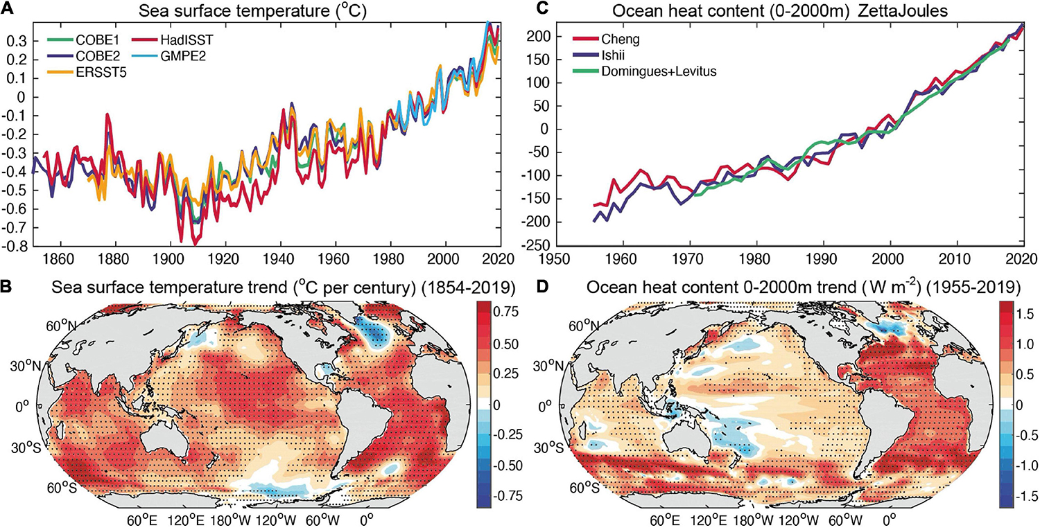
Figure 1. (A) Global mean SST time series from1850 to 2019 (°C). Five datasets are used, including: COBE1, COBE2, ERSST5, HadISST, and GMPE. (B) Spatial distribution of the long-term SST trend from 1854 to 2019 for ERSST data (°C per century). (C) Global ocean heat content changes for the upper 2,000 m, three time series are provided (Domingues et al., 2008; Levitus et al., 2012; Cheng et al., 2017; Ishii et al., 2017). The Domingues estimate (0–700 m) is combined with the Levitus estimate (700–2,000 m) to produce a 0–2,000 m time series, according to IPCC (Rhein et al., 2013). The energy unit is the ZettaJoule (10²¹ Joules). (D) Spatial distribution of long-term ocean heat content trend (0–2000m) (W m^{− 2}) for Cheng et al. (2017) data. All data are annual mean time series and use a 1981–2010 baseline. Black dots (in b and d) indicate grid boxes where trends are significant at a 90% confidence interval.

In each dataset, the 10 warmest years on record have all occurred since 1997, with the five warmest years occurring since 2014. The recent decade (2010–2019) shows a much higher rate of warming than the long-term trend: 0.287 ± 0.144 (COBE1), 0.270 ± 0.160 (COBE2), 0.240 ± 0.150 (HadISST), 0.323 ± 0.168°C per decade (ERSST). The mean rate is 0.280 ± 0.068°C per decade within 2010–2019. Figure 1A has been provided to graphically illustrate the changes to SST since ∼1850.

By regions, sea surface warming appears in most of the ocean areas (Figure 1B), which is an unequivocal signal of human-induced climate change (Bindoff et al., 2013). However, in the North Atlantic Ocean, it shows a long-term cooling trend (called the cold blob or North Atlantic warming hole), which extends from the sea surface to 2,000 m deep. Many studies indicate that this warming hole is a footprint of the AMOC (Caesar et al., 2018).

Ocean Heat Content

Because of the emission of heat-trapping greenhouse gases by human activities, the natural energy flows have been interfered and currently there is an energy imbalance in the Earth’s climate system (Hansen et al., 2011; Trenberth et al., 2014; von Schuckmann et al., 2016, 2020). More than 90% of the excess heat is accumulated within the global oceans (Rhein et al., 2013) thus leading to an increase in ocean heat content (OHC). OHC is a fundamental indicator of global warming (Hansen et al., 2011; von Schuckmann et al., 2016; Wijffels et al., 2016; Cheng et al., 2018a; Trenberth et al., 2018). Compared with SST and global mean surface temperature records, the OHC record shows larger signal-to-noise ratio and is less impacted by natural variability (Wijffels et al., 2016; Cheng et al., 2018a,b). Therefore, OHC is better suited to detecting and attributing human influences than other climate records.

The first global OHC time series was provided by Levitus et al. (2000), where a robust long-term 0–3,000 m ocean warming was identified over the 1948–1998 period. Since 2000, a number of global and regional OHC data sets have been made available (Willis et al., 2004; Ishii et al., 2005; Palmer et al., 2007; von Schuckmann and Le Traon, 2011; Levitus et al., 2012; Lyman and Johnson, 2013; Desbruyères et al., 2017; Cheng et al., 2017; Zanna et al., 2019). However, the early global OHC time series show significant decadal variability, specifically, a warm period from the 1970s to the early 1980s. This pattern is not reproducible by climate models (Domingues et al., 2008). In 2007, Gouretski and Koltermann (2007) found that the time variation of the systematic errors in expendable bathythermographs (XBT) data is largely responsible for this decadal variation in OHC time series. Since then, scientific community efforts have been aimed to understand XBT errors and improve data quality. Scientific community consensus was developed in 2016 for the best practice of the correction of XBT bias (Cheng et al., 2016). After correcting the systematic errors, the XBT data quality has been improved and the OHC time series show a more homogeneous warming in the half century (Cheng et al., 2018a,b; Goni et al., 2019). In addition to the XBT error, several other sources of uncertainty in OHC estimates have been identified, including MBT biases (Gouretski and Cheng, 2020), mapping methods, and choice of climatology etc. Boyer et al. (2016) found that the major source of error in OHC estimates is the mapping method, which defines how the global map of a variable is created from incomplete observations and how the reconstructed field is smoothed.

It is becoming increasingly clear that many traditional gap-filling strategies introduced a conservative bias toward low-magnitude changes (Durack et al., 2014). To improve how spatial gaps are accounted for in historical ocean temperature measurements Cheng et al. (2017) proposed a new spatial interpolation method. Ishii et al. (2017) suggested a correction to their previous estimate. Based on these developments, we used three less-biased OHC estimates (here “less biased” means the global time series are less biased to the conservative error. This does not indicate that their regional signals are less biased), including Domingues et al. (2008); Cheng et al. (2017), and Ishii et al. (2017).

Estimates show highly consistent ocean warming since the late 1950s. Figure 1C provides data on ocean warming (down to a 2,000 m depth). The results reveal a linear warming rate of 0.36 ± 0.06 (Ishii et al., 2017), and 0.34 ± 0.10 (Cheng et al., 2017) Wm^–2 over the 1955–2019 period (averaged over the Earth’s surface), with the mean rate of 0.35 ± 0.08 Wm^–2. The new estimates are collectively higher than previous estimates (Rhein et al., 2013) and more consistent with each other (Cheng et al., 2019b). The past 10 years are the ten warmest on record for OHC (Cheng et al., 2019b).

The rate of ocean warming for the upper 2,000 m has increased since the 1990s, with linear trends of 0.59 ± 0.03 Wm^–2 (Cheng et al., 2017), 0.57 ± 0.06 Wm^–2 (Ishii et al., 2017), and 0.66 ± 0.02 Wm^–2 (Domingues et al., 2008; Levitus et al., 2012) over 1990–2019. The mean rate during this period is 0.61 ± 0.05 Wm^–2. For the period 2010–2019, the rate of OHC increase is: 0.65 ± 0.07 Wm^–2(Cheng et al., 2017), 0.79 ± 0.08 Wm^–2 (Ishii et al., 2017), and 0.66 ± 0.03 Wm^–2 (Domingues et al., 2008; Levitus et al., 2012). The mean rate is 0.70 ± 0.07 Wm^–2. The latest data show that the upper 2,000 m of the world’s oceans continued a trend of breaking records in 2020. Each of the last six decades have been warmer than the previous decade (Cheng et al., 2021).

Increases in OHC are evident throughout the global ocean from the surface down to 2,000 m over the 1960–2019 period (Figures 1D, 2). There are some interesting local patterns for long-term OHC change. There has been stronger warming in the Southern Ocean (70°S∼40°S) and Atlantic Ocean (40°S∼50°N) than other regions and weaker warming throughout the Pacific and Indian Oceans (30°S∼60°N). Models suggest that the Southern Ocean has taken up most of the global warming heat in the past century (Cheng et al., 2017; Swart et al., 2018), driven predominantly by air-sea flux changes associated with upper-ocean overturning circulation and mixing (Swart et al., 2018). Despite of the broad scale 0–2,000 m ocean warming, the subtropical regions in the southwest Pacific and Indian oceans (near the eastern Australia coast and Madagascar), which extends from ∼200 to 1,000 m have displayed a different trajectory. The formation of these cooling signals has not been well understood before.

FIGURE 2

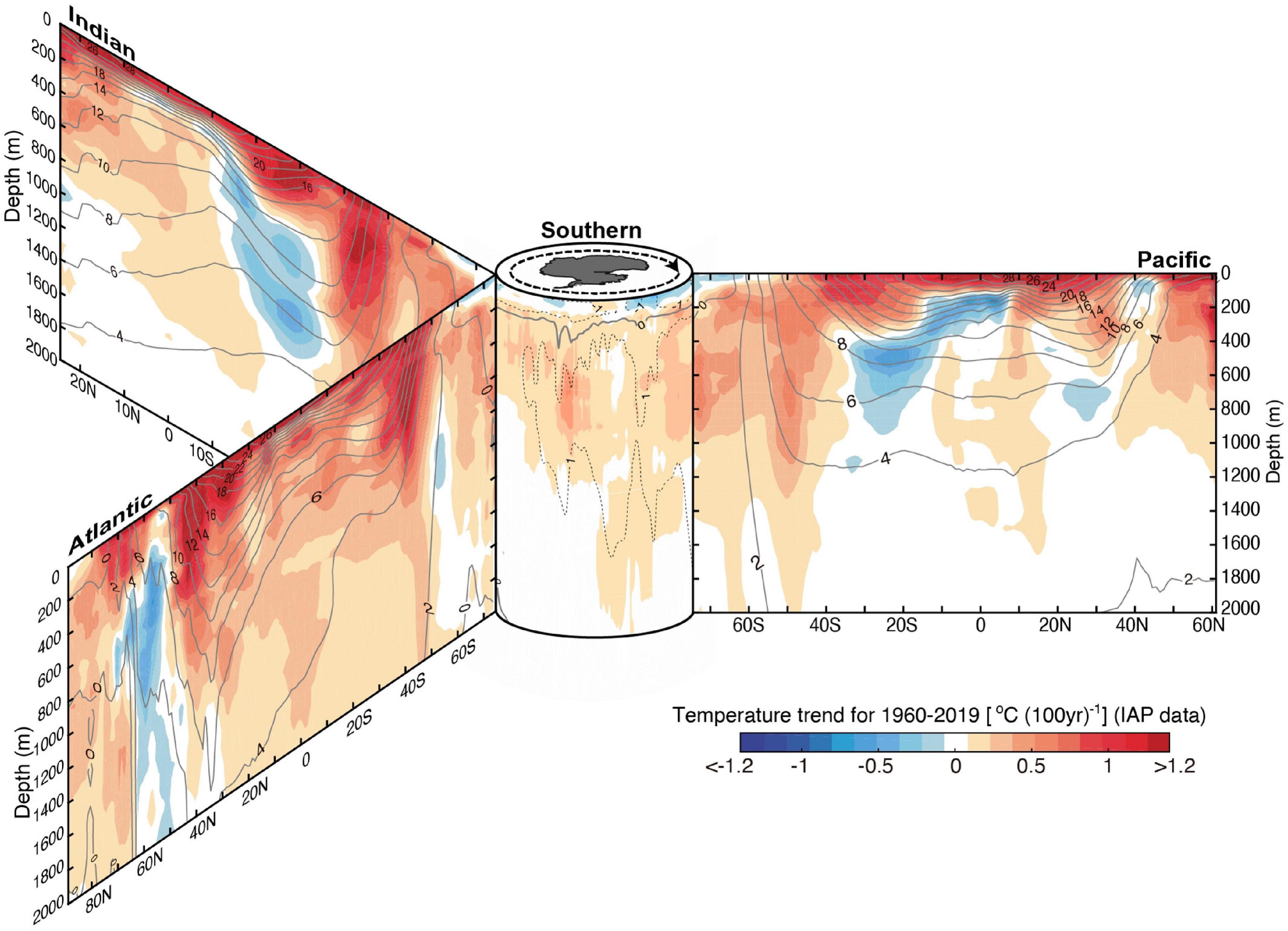
Figure 2. Vertical section of the ocean temperature trends (°C per century) from the sea surface to 2,000 m depth in the period 1960–2019 (60-year ordinary least-squares linear trend). Shown are the zonal mean sections in each ocean basin organized around the Southern Ocean (south of 60°S) in the center. Black contours show the associated climatological mean temperature with intervals of 2°C (in the Southern Ocean, 1°C intervals are provided in dashed contours). Figure from Cheng et al. (2020).

The Period 1998–2013

A slowdown in the increase of SST and global mean surface temperature has been observed from 1998 to 2013 and led to numerous assertions about a “global warming hiatus” (Hartmann et al., 2013). It has been increasingly clear that this temporal slowdown in surface temperature change is caused by a combination of internal variability, external forcing and the bias in data (Meehl et al., 2011; Kosaka and Xie, 2013; England et al., 2014; Santer et al., 2014; Schmidt et al., 2014; Watanabe et al., 2014; Foster and Abraham, 2015). In particular, there are substantial interannual and decadal scale variability in surface records, which reduces the signal-to-noise ratio of these records. Consequently, a longer time is required to detect a robust trend from surface indicators compared to subsurface or integrated indicators such as OHC and sea level rise. The SST record until 2019 (Figure 1A) shows that the linear trend of SST for 1998–2019 is 0.137 ± 0.061°C per decade, greater than the linear trend during the previous decades (1982–1997; 0.100 ± 0.046°C per decade). This range includes the appearance of the extreme 2015/16 El Niño event (Hu and Fedorov, 2017). The rate of OHC increase has been more than doubled since 1990 (Figure 1C). The continuous increase in the rate of SST and OHC refute the concept of a slowdown of human-induced global warming (Gleckler et al., 2016; Cheng et al., 2020).

Global Surface Ocean pH

Ocean acidification is the anthropogenic reduction in the pH of the ocean over an extended period of time, decades to centuries. The ocean has absorbed about 25% of all CO₂ emissions (1870–2015 period; Le Quéré et al., 2018; Gruber et al., 2019a,b; Friedlingstein et al., 2020) and the increased CO₂ in the water is lowering its pH through the formation of carbonic acid (Figure 3). Increased aqueous CO₂ is also leading to an increase in bicarbonate and decrease in carbonate ions.

FIGURE 3

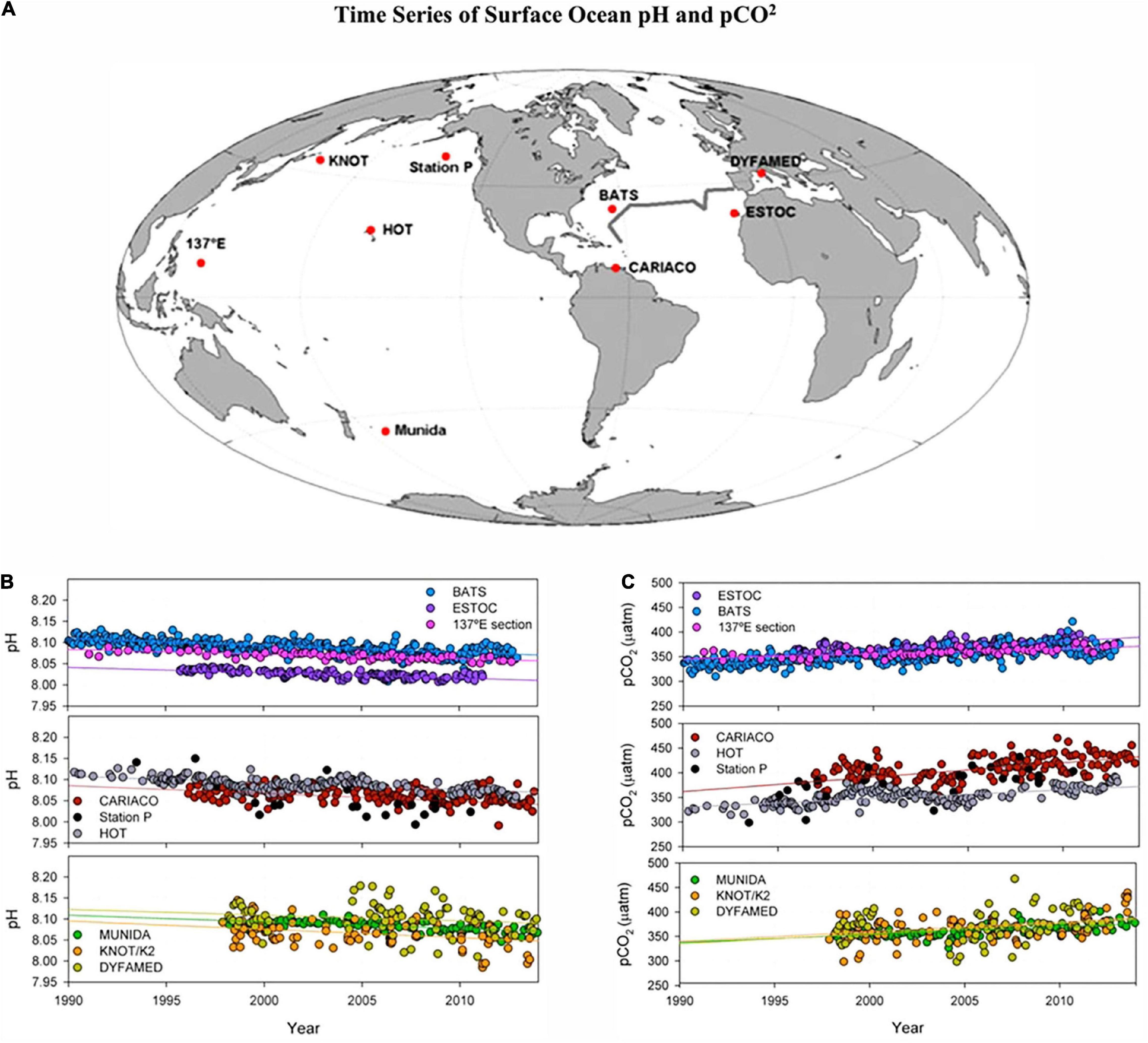
Figure 3. Trends in surface (<50 m) ocean carbonate chemistry calculated from observations obtained at global monitoring stations. (A) Positions of time-series stations (red dots). (B) Time series of deseasonalized surface ocean pH measurements and trend lines. pH is on total scale for in-situ temperatures. (C) Time series of deseasonalized surface ocean pCO2 measurements and trend lines. Figure from Tanhua et al. (2015).

Global surface ocean pH has declined on average by approximately 0.1 (from 8.2 to 8.1) since the Industrial Revolution (Caldeira and Wickett, 2003; Orr et al., 2005). Jiang et al. (2019) reports a similar global decrease of −0.11 ± 0.03 pH units from 1770 to 2000. The Arctic Ocean has experienced the largest pH decrease with a pH decline of −0.16 ± 0.04 pH units (1,770–2,000). There is natural variability of the ocean’s carbonate chemistry driven by a number of natural processes such as circulation, air-sea interchange, and remineralization for example, but carbonate chemistry at global scale is being driven by the increasing carbon dioxide in the atmosphere coming from emissions and land use change. The current changes can be observed in extended ocean time series and the rate of change is likely unparalleled in at least the past 66 million years (Hönisch et al., 2012; Zeebe et al., 2016). Ocean pH is projected to decline, approximately, by an additional 0.1–0.4 pH units by the end of century (2,100) depending on the future RCP (Representative Concentration Pathway) / SSP (Shared Socioeconomic Pathways) scenarios (Caldeira and Wickett, 2003; Feely et al., 2009; Jiang et al., 2019; Kwiatkowski et al., 2020).

Carbonate chemistry varies according to large-scale oceanic features including depth, distance from continents due to land influence, upwelling regime, freshwater/nutrient input and latitude (Jewett and Romanou, 2017). Due to this variability, as determined by these various characteristics, only longer term, observational time series can detect the predicted long-term increase in acidity at individual sites due to rising atmospheric CO₂ levels. Time of emergence of the signal varies from 8 to 15 years for open ocean sites, and 16 to 41 years for coastal sites (Sutton et al., 2019), making it necessary to commit to long-term observational records, especially in the coastal zone where most commercially and culturally important marine resources reside.

Dissolved Oxygen Concentration

The ocean can only gain oxygen at the surface by air sea gas exchange and photosynthesis. Subsurface dissolved oceanic oxygen (DO) is advected along water mass distribution pathways and mixed into adjacent water masses while being consumed by respiration. Therefore, any change in solubility at the surface (due to warming), decrease of ventilation (due to stratification increase) and increase in deep ocean respiration (due to increased surface primary production and enhanced particle flux) can lead to oceanic deoxygenation. Thus, changes in deep ocean DO can be seen as an integrative long-term indicator for profound changes in physical or biogeochemical ocean dynamics.

Since oxygen is the marine biogeochemical parameter with little to no variations in analysis methods over time, long-term oceanic DO changes can be derived robustly with relatively high confidence (Carpenter, 1965; Wilcock et al., 1981; Knapp et al., 1991). Only limited data availability may compromise robust trends in all regions and depths. Winkler titration of water samples, established in 1903, has become the method of choice for DO measurements soon after its discovery and has since been used to calibrate DO measurements of all kind of platforms. More recent developments of computer-aided Winkler titration methods that provide higher accuracy, seem not to bias historical measurements (Schmidtko et al., 2017). Furthermore, a systematic relative bias due to reagent changes in the analysis was tested and determined as highly unlikely (Schmidtko et al., 2017). Therefore, any calibrated long-term DO observation can be used to derive long term trends and multi-decadal variability of timeseries spanning a century.

Coastal changes in DO are impacted on a very local scale by regional physical, biogeochemical and anthropogenic changes. These regional changes range from riverine run-off of nutrients, deposits of organic matter over heatwaves and tides, just to name a few. An observational study (Diaz and Rosenberg, 2008) reports an increased occurrence of coastal dead zones, with consequences for regional ecology and economy. While the occurrence of most of these coastal dead zones is locally driven, some low-oxygen events may have been affected by open ocean deoxygenation, making these events more likely by lowering background DO levels.

In the open ocean most long-term time series data from monitoring stations show decreasing DO levels despite temporal variations on annual to multidecadal time-cales (e.g., Keeling et al., 2010). Time stations with long-term increasing oxygen levels exist but are sporadic.

The long term monitoring stations support the findings of three major studies of global DO changes, covering the time period from the sixties to today (Helm et al., 2011; Ito et al., 2017; Schmidtko et al., 2017). Figure 4 shows an overview of the relevant changes. Despite diverging methods all studies agree that the global ocean is losing oxygen at a significant rate. The rate of decrease does vary over depth and method but is on the order of 2% over 50 years (Schmidtko et al., 2017). This accumulates to a loss of 4.8 ± 2.1 petamoles since 1960. This loss is not homogeneously distributed in the global ocean. Oceanic oxygen loss varies with depth and region, resembling the several processes involved in oxygen distribution and consumption. All the works generally agree on the large scale deoxygenation patterns with most pronounced deoxygenation in the north Pacific and Southern Oceans with some smaller disagreement regarding the intensity of deoxygenation in the tropical oceans.

FIGURE 4

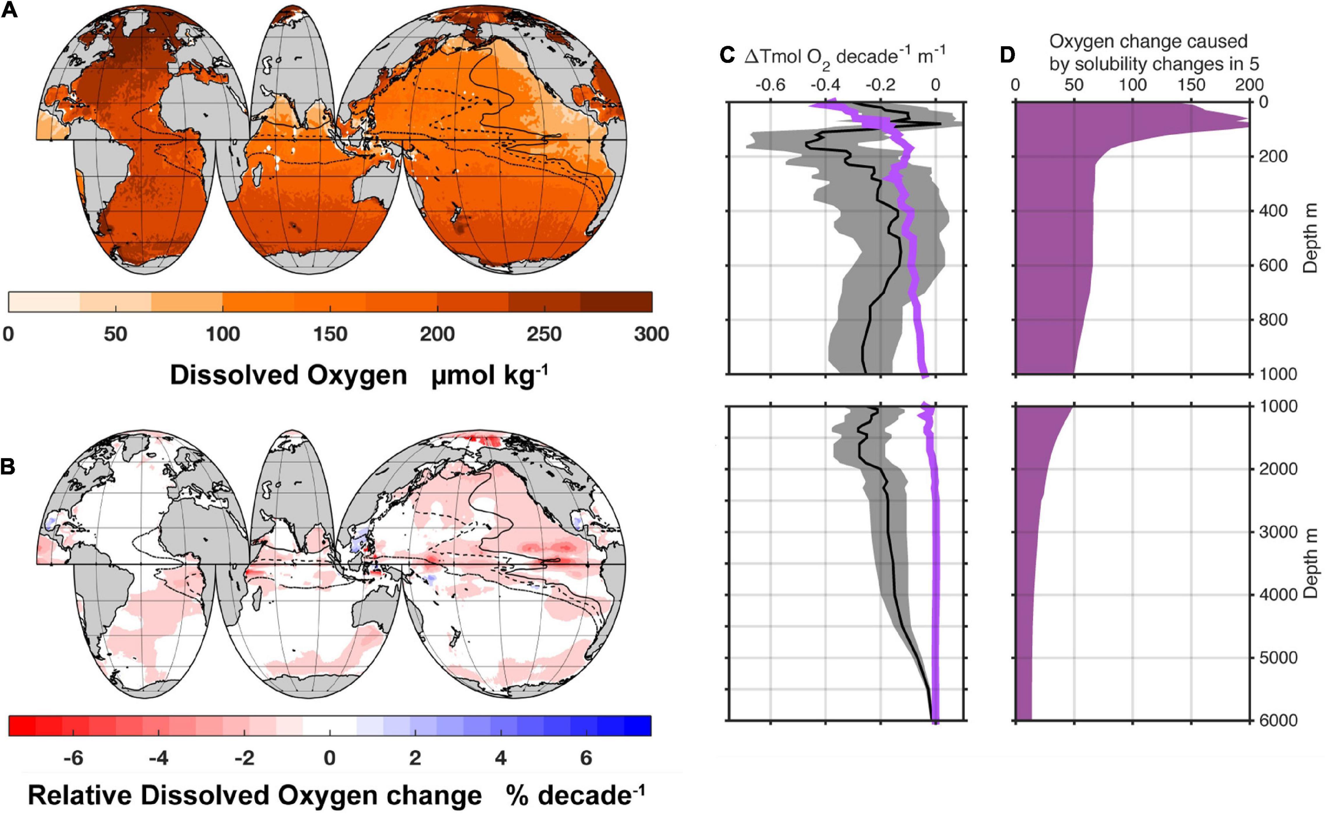
Figure 4. Spatial and temporal trends of dissolved oxygen concentration. (A) Mean oxygen concentration, lines indicate the maximum extent of the oxygen minimum zone with 40, 80, and 120 μmol kg^{− 1} dissolved oxygen anywhere in the water column. (B) Trend of oxygen over five decades 1960–2010 (A,B) data from Schmidtko et al., 2017. (C) Vertical distribution of deoxygenation (black curve) and error (gray area), the purple line indicates the loss expected from oceanic warming detected in the same data set. (D) Percentage of deoxygenation due to warming for the water column, values above 100% indicate that processes counter acting solubility deoxygenation are at play (C,D) (reworked from Schmidtko et al., 2017).

From a global perspective, temperature-driven solubility decrease is dominating the oxygen loss in the upper most water layers. A warming ocean is gaining less oxygen from air sea gas exchange. Schmidtko et al. (2017) attribute 50% of the oxygen loss in the upper 1,000 m to solubility changes. This number drops to about 25% for the upper 2,000 m and only on the order of 13% of the overall full water column oxygen loss. This solubility driven deoxygenation is attributed to the time period 1960–2010, assuming linear warming. For an accelerating warming process these numbers will likely change. Since solubility is responsible for only part of the observed changes, other processes are similarly important. Nevertheless, we cannot disregard temperature as the key source of those changes as well, since processes other than solubility change are also largely driven by a warming upper ocean. These temperature driven processes are not limited to, but do include stratification increase, circulation changes and thermal impacts on biogeochemical cycles (e.g., Keeling and Garcia, 2002; Stendardo and Gruber, 2012; Bianchi et al., 2013).

More recent analysis of available regional studies (Stramma and Schmidtko, 2021) attribute various processes to observed regional changes (Figure 5). While solubility and stratification dominate high latitudes and the Atlantic Ocean, multi-decadal variability is dominant throughout most basins. The reason for this can be seen in atmosphere-ocean indices like the North Atlantic Oscillation (NAO), El Nino-Southern-Oscillation (ENSO), and Pacific Decadal Oscillation (PDO), among many others, impacting regional ocean dynamics with subsequent influences on dissolved oceanic oxygen. Biological and nutrient stimulation causes are mainly found near the coast and in particular upwelling regions. Source water changes and circulation driven changes point to physical parameters that have shifted in ocean dynamics. Many of these processes are linked to changing ocean ventilation and respiration and are therefore challenging to appraise directly. Still, all tend to reinforce the impacts from warming (Oschlies et al., 2018).

FIGURE 5

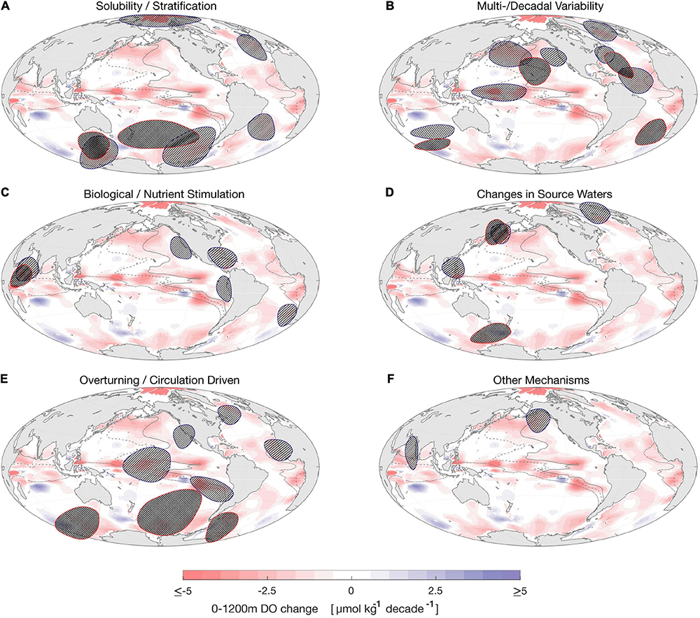
Figure 5. Major drivers of regional oxygen variability marked as approximate areas as described in peer-reviewed articles from observations and model analyses (see details in Stramma and Schmidtko, 2021). Background colors indicate upper ocean oxygen changes in μmol kg^{− 1} decade^{− 1}. The areas with significant variability from (A) solubility and/or stratification, (B) multi-decadal or decadal variability, (C) biological and/or nutrients stimulation, (D) changes in source waters, (E) overturning and/or circulation driven, and (F) other mechanisms. The diagonal-hatched regions indicate upper ocean impact, the cross-hatched regions indicate deep ocean variability. (reworked after Stramma and Schmidtko, 2021).

Along with globally decreasing oceanic DO, the volume of so-called oxygen minimum zones has grown significantly. Oxygen minimum zones (OMZ) are generally defined as oceanic volume with less than 80 mmol l^–1 DO, and thus not suited as habitat for many marine organisms that rely on continuous respiration although they may provide refuge for animals that can cope with low DO conditions. In areas where the OMZ DO levels are close to or completely depleted oxygen minimum zones have potential impacts on greenhouse gas driven climate warming, since they can emit large quantities of nitrous oxide, a potent greenhouse gas, owing to denitrification processes under anoxic conditions (e.g., Codispoti, 2010; Santoro et al., 2011). Such low OMZ DO levels can be found in the Pacific and Indian Ocean and have been found expanding.

With impacts on dissolved oxygen levels varying strongly on regional scales, predictions on future local oxygen can only be established knowing all local boundary conditions and predicted changes. At basin scale or even global scale, it can be stated that an increased warming of the upper ocean has impact on oxygen levels by solubility while simultaneously reinforcing other processes that are linked to ocean dynamics and biogeochemistry, and that are responsible for the majority of the observed deoxygenation.

Arctic Sea Ice Extent, Thickness and Volume

The retreat of Arctic sea ice has been one of the most iconic indicators of climate change (Thoman et al., 2020). Arctic sea ice extent is declining by −13.1% per decade during summer (September 1979–2020), when it exhibits its seasonal minimum extent, and by −2.6% per decade during winter (March 1979–2018) (Fetterer et al., 2017; Perovich et al., 2020). Figures 6A,B present the mean sea ice concentration in summer and winter during the last 4 decades and Figures 6C,D the sea ice concentration trends during the same period and seasons. The decreasing trends during winter (Figure 6C) are observed in all the peripheral seas around the Arctic, with the greatest decreasing trends (−26% per decade) occurring in the Barents Sea. During summer the trends (Figure 6D) are almost twice as high in the Pacific and Asian sectors of the Arctic Ocean compared to the Atlantic Sector, with the greatest decreasing trends occurring in the Beaufort Sea (−29% per decade), which has been essentially ice free during summer over the past decade. The record minimum in summer sea ice extent was measured in September 2012, and the second lowest extent in the 42 years satellite record was measured in September 2020 (Perovich et al., 2020).

FIGURE 6

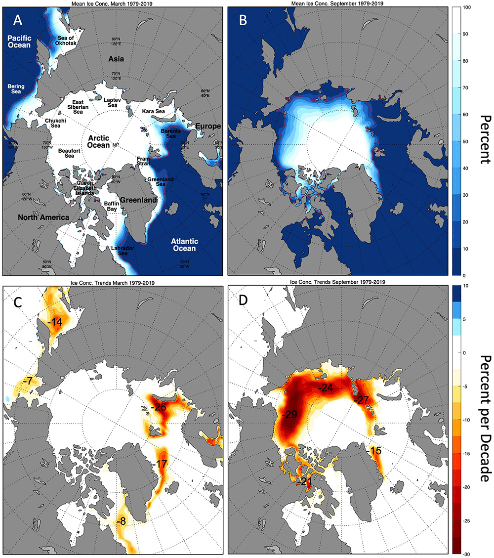
Figure 6. Arctic Mean Sea Ice Concentration (percent) during the last 4 decades (1979–2019) in winter (March; A) and summer (September; B); and Arctic Sea Ice Concentration Trends (percent per decade) in winter (March; C) and summer (September; D) during the same 40 year period (1979–2019) estimated from Bootstrap Sea Ice Concentration analysis (https://nsidc.org/data/nsidc-0079/versions/3; Comiso, 2017).

Similarly, the thickness of Arctic sea ice has also decreased. In one of the first studies to document this change, using measurements from upward looking sonars on submarines, Rothrock et al. (1999) showed that the average of thickness of sea ice decreased from 3.1 meters in 1958–1976, to just 1.8 meters in 1993–1997, with the largest decreases occurring in the central and eastern Arctic. In an updated study which includes estimates of sea ice thickness from satellites, Kwok (2018) showed that the thickness has now decreased by 2.0 meters, comparing 2011–2018 ICESat and CryoSat-2 data to the 1958–1976 and 1993–1997 submarine cruise measurements, or about 66% over the six decades.

Taken together, the observed trends in sea ice extent and sea ice thickness indicate that the volume of Arctic sea ice has decreased by over 75% since 1979. This estimate is coincident with many modeling studies, including the Pan-Arctic Ice Ocean Modeling and Assimilation System (Zhang and Rothrock, 2003; Schweiger et al., 2011, 2019) which estimates that the average volume of Arctic sea ice of 11.5 × 10³ km³ in September, 1979–2010, has decreased with a rate of −2.8 × 10³ km³ per decade. The current record minimum in total ice volume estimate using PIOMAS is 3.8 × 10³ km³ set in September 2012. The summers of 2019 and 2020 are tied for second minimum with 4.2 × 10³ km³.⁵

These trends in the decline of Arctic sea ice are the result of the complex interplay between the atmosphere, sea ice and the ocean. During the winter, the cold halocline layer protects sea ice from the underlying warm Atlantic water (e.g., Steele and Boyd, 1998), allowing sea ice to grow thermodynamically driven by air temperatures which historically were around −32°C (Rigor et al., 2000). Winds and ocean currents may also change the thickness of sea ice dynamically by ridging and rafting of sea ice during storms or against a coastline. This process also creates areas of open water which would rapidly freeze over and thicken during winter, quickly increasing the thickness distribution of sea ice. Most of the sea ice in the Arctic Ocean is exported through Fram Strait, and later melts in the warmer waters of the Greenland Sea and North Atlantic. Heat from the atmosphere also melts sea ice on the Arctic Ocean during summer.

The global trends in air temperature are more dramatic in the Arctic due to the ice-albedo feedback and Polar Amplification of global warming (e.g., Manabe and Stouffer, 1980). As warmer temperatures melt the ice, the lower albedo of the surface allows more heat to be absorbed by the surface leading to a positive feedback that amplifies the global warming signal. Changes in wind related to the Arctic Oscillation (AO, Thompson and Wallace, 1998) have also been linked to the decline of sea ice. For example, Rigor et al. (2002) have shown that during high AO winters the winds blow more sea ice away from the Eurasian coast which allows more heat from the ocean to warm the atmosphere over these areas. Rigor and Wallace (2004) found that the trends in sea ice extent during summer (e.g., Figure 6D) are a lagged response, specifically, the younger, thinner sea ice that develops along the Eurasian coast during high AO winters, is less likely to survive the summer melt. The younger, thinner sea ice pack is also blown faster by the winds and is more prone to fracturing and increasing amounts of open water and leads during all seasons, allowing more heat to be released by the ocean during winter, and more heat to be absorbed by the ocean during summer, which will delay freeze up. Thus the increased kinematics of sea ice provides a dynamic complexity that strengthens the ice-albedo feedback even more (Rampal et al., 2011).

The high Arctic Oscillation conditions may have also shifted the ocean currents so that river runoff from the Eurasian continent was diverted to the east, weakening the cold halocline later and allowing heat in the Atlantic waters to reach the surface and melt sea ice (Morison et al., 2012, 2021). Polyakov et al. (2020) show that the weakening of the cold halocline layer is also observed in in the Eurasian Basin through 2018 and estimate that the Atlantic waters heat increased to over 10 Wm^–2 in 2016–18 (from 3–4 Wm^–2 in 2007–2008), decreasing winter ice growth by twofold.

Global Mean Sea Level

The IPCC Special Report on Oceans and Cryosphere (SROC, Oppenheimer et al., 2019) concluded that the rate of change of the Global Mean Sea Level (GMSL) was, respectively, 1.4 and 3.2 mm year^–1 for the periods 1901–1990 and 1993–2015. Several studies have advanced the analysis of the trend of GMSL by improving the accuracy of the observational data adding observations by different platforms, using different analysis methods, reconstructing time series, or using climate models to simulate the sea level evolution. By means of a novel hybrid sea-level reconstruction applied to the global tide gauge time series Dangendorf et al. (2019) estimated a GMSL trend of 1.6 mm year^–1 from 1900 to 2015, an increase of 0.19 m since 1900. From the analysis of altimetry for the period 1993–2017 Nerem et al. (2018) observed a GMSL rise of 2.9 ± 0.4 mm year^–1 and an acceleration of 0.084 ± 0.025 mm year^–2. Dangendorf et al. (2019) also found a notable increase in the GMSL rate from 1993 (2.1 mm year^–1) to 2015 (3.4 mm year^–1) and a persistent acceleration of 0.06 mm year^–2 since the 1960s. Cazenave et al. (2019) using the most recent time series (January 1993–February 2019) gives a mean rate of sea level rise of 3.15 ± 0.3 mm year^–1, with an acceleration of 0.10 ± 0.04 mm year^–2. This acceleration value agrees well with Nerem et al. (2018)’s estimate. GMSL is projected to rise by the end of the century (2100) between 0.43 m (0.29–0.59 m) under RCP2.6 and 0.84 m (0.61–1.10 m) under RCP8.5 and will continue to increase during centuries due to ocean heat uptake and the melting of the ice sheets and glaciers (Oppenheimer et al., 2019).

Sea level trend maps computed from satellite altimetry data reveal that even though a general GMSL rise has occurred during the altimetry era, the MSL change follows regional and local variability with diferences up to 8 mm year⁻¹ reflecting the pattern of ocean currents, the large-scale oceanic and atmospheric oscillations or the contribution of the melting ice-sheets among other factors (Figure 7). Basin-scale MSL trend variability is also observed from the longer tide gauges series (e.g., Slangen et al., 2017; Dangendorf et al., 2019). For the period 1900–2018, Frederikse et al. (2020) found a positive MSL trend in all the ocean basins, being the highest for the subtropical North Atlantic (2.49 mm year^–1) and south Atlantic (2.07 mm year^–1), the lowest for the subpolar North Atlantic (1.08 mm year^–1) and East Pacific (1.20 mm year^–1), while intermediate values were observed in the Indian-south Pacific (1.33 mm year^–1) and in the northwest Pacific (1.68 mm year^–1).

FIGURE 7

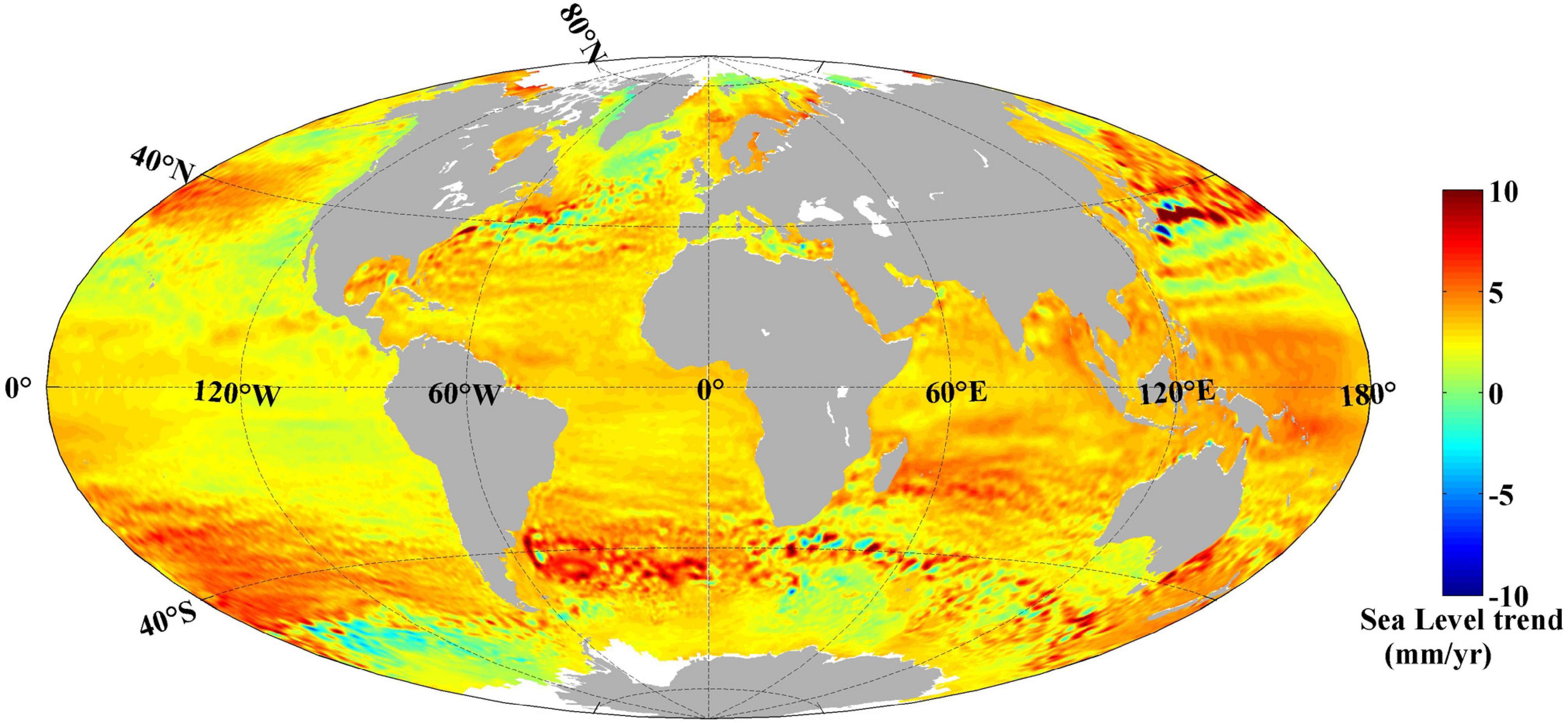
Figure 7. Map of sea level trends (mm yr⁻¹) elaborated using 27 years of satellite multi-mission altimetry data (January 1993–October 2019). Credits EU Copernicus Marine Service (CMS).

Separating the global drivers of the MSL variability at a regional scale and even more at a local scale, becomes complex. In addition to the anthropogenically forced sea-level signal, the internal variability is time and location-dependant (Stammer et al., 2013). Thus, large atmospheric and ocean oscillations (e.g., El Niño Southern Oscillation, Pacific Decadal Oscillation, North Atlantic Oscillation, Indian Ocean Dipole) have interannual and decadal signals in MSL time series being of different period and intensity depending on the ocean basin. Analyzing the MSL trend from a regional perspective additionally allows development of a more detailed characterization of the global sea level budget. For instance, from a hybrid MSL reconstruction from 1900 to 2015, Dangendorf et al. (2019) demonstrate that a great part (∼76%) of the GMSL acceleration from the 1960s has its origin in the Indo-Pacific (0.07 ± 0.01 mm year^–2) and South Atlantic sea (0.06 ± 0.01 mm year^–2) as a consequence of an intensification and a displacement of the southern hemispheric westerlies that contributed to increased heat uptake and consequently a more intense thermal expansion.

With regard to local MSL trends, besides the complex processes occurring near the coast (e.g., Benveniste et al., 2019), and the particular importance of land subsidence, the different scale processes contributing to the sea level variability has not only a local origin, but it can be generated far away (Woodworth et al., 2019). The IPCC Special Report on Oceans and Cryosphere (Oppenheimer et al., 2019) further indicates that the local Extreme Sea Level (ESL) events happening once in one hundred years will become annual events in many low-lying cities and small islands by 2050 under all RCP scenarios due to the projected Global Mean Sea Level Rise (GMSL).

The Strength of the Atlantic Meridional Overturning Circulation (AMOC)

Direct continuous measurements of the AMOC only started in 2004 with RAPID-MOCHA (Smeed et al., 2014), an array of moored instruments that spans the width of the Atlantic at latitude 26.5 degrees north and provides continuous monitoring of the AMOC. Before, there had only been five individual snapshots of the AMOC, computed from seawater density measurements taken at hydrographic sections in the years 1957, 1981, 1992, 1998, and 2004 (Frajka-Williams et al., 2019). A couple of other trans-basin observing arrays at different locations in the Atlantic followed, including SAMBA in the South Atlantic in 2009 (Meinen et al., 2018) and OSNAP in the subpolar North Atlantic in 2014 (Li et al., 2017).

The RAPID observations recorded a notable decrease of 2.7 Sverdrup (Sv; 1 Sv = 10⁶ m³ s^–1), about 15%, in AMOC strength between April 2004 until roughly April 2008, followed by a fairly stable period until the end of the recovered data in September 2018 (Smeed et al., 2018; Moat et al., 2020). Yet such a short record cannot distinguish between decadal variability and long-term slowdown. Various studies have attempted to reconstruct the AMOC for the time period before 2004 using other climatic variables, so-called proxies, like sea surface temperatures (Latif et al., 2006; Rahmstorf et al., 2015) and sea level heights (Frajka-Williams, 2015) as well as the available snapshots (Bryden et al., 2005; Kanzow et al., 2010). Using the latter Bryden et al. (2005) estimated a decrease in AMOC transport at 26°N of about 30% between 1957 and 2004. Two main criticisms were levied against this conclusion. One, the first 4 years of the observed overturning strength provided by the RAPID data (Kanzow et al., 2010; Smeed et al., 2014) suggested that the seasonal variability of the AMOC has an amplitude of several Sverdrup, significantly larger than previously thought, thus, the five snapshots used by Bryden et al. (2005) might have sub-sampled intense high-frequency variability, rather than a robust trend. Correcting the measurements for the seasonal cycle Kanzow et al. (2010) found a much smaller weakening of only 13%. A different approach, estimating the strength of the AMOC mainly from the more widely available measurements of CTD (Conductivity-Temperature-Depth) end stations, found a reduction of about 2–4 Sv between 1980 and 2005, but concluded that this trend cannot be statistically validated due to the large variability in the layer transports found in the data (Longworth et al., 2011). This is in direct opposition to the findings of Latif et al. (2006) who concluded from the observed linear trend in the sea surface temperatures in the North Atlantic that the AMOC has strengthened since 1980. Combining the observed density change in the region of the Denmark Straight with the results from ocean model simulations they estimated the increase to be about 1 Sv between 1970 and 2000. These seemingly contradictory results could be reconciled with the AMOC reconstruction by Caesar et al. (2018), based on the relative cooling in the subpolar North Atlantic, who see a decline of AMOC strength since the 1950s with a short-lived recovery that is evident in the 1980s and 90s before a return to decline from the mid-2000s (Figure 8). This short-lived recovery of the AMOC is also found by Jackson et al. (2016) by analyzing a global-ocean reanalysis product, the GloSea5 data, which covers the years 1989–2015 as well as by Frajka-Williams (2015) who combined sea surface height data from satellites with cable measurements to reconstruct the AMOC from 1993 to 2014. Caesar et al. (2018), found an overall decline of the AMOC of about 3 ± 1 Sv (about 15%) since the mid-twentieth century.

FIGURE 8

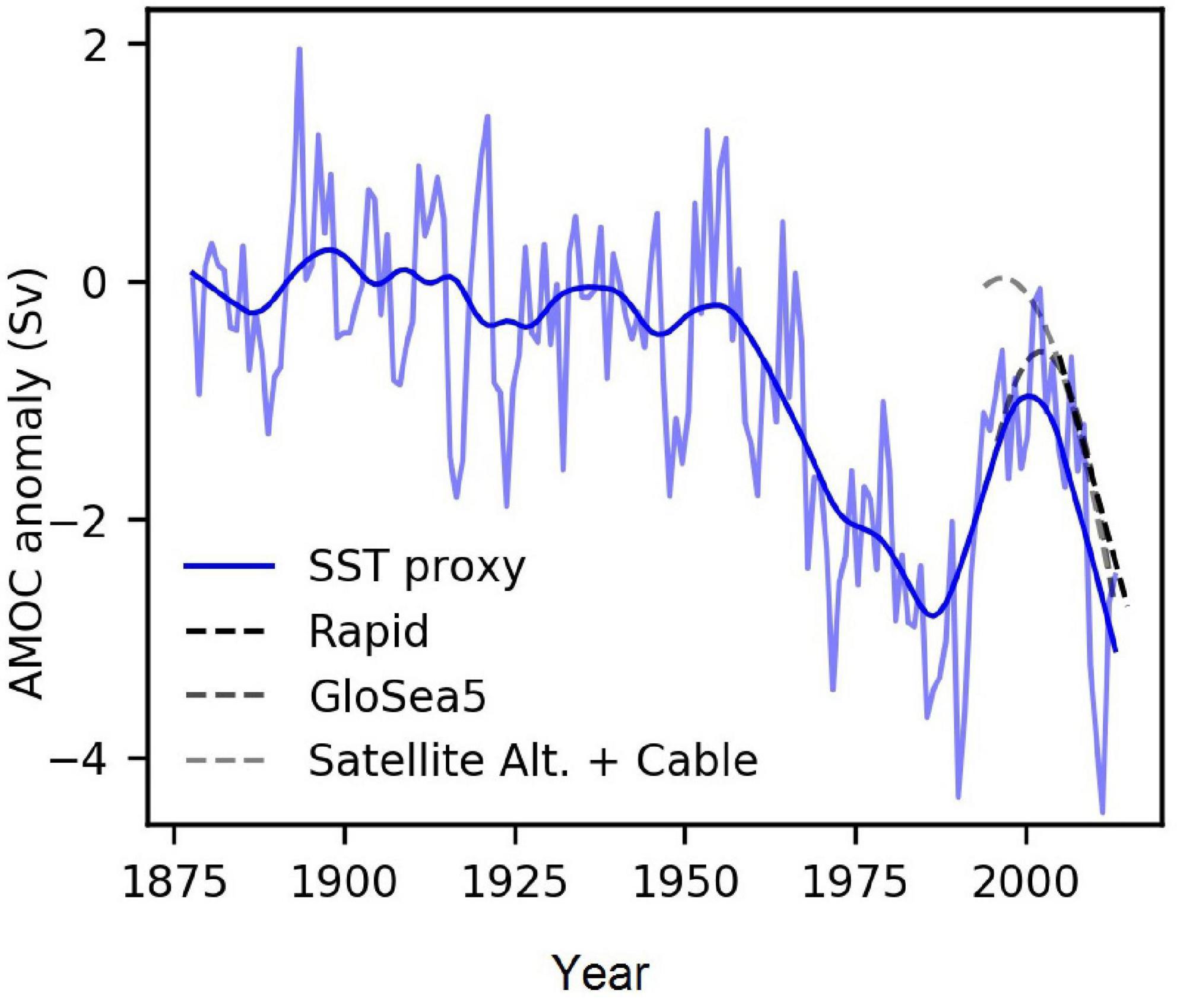
Figure 8. Trend of the strength of the overturning circulation (AMOC) in observations. Shown are (i) the long-term (20-year LOWESS filtering, thin line are annual values) sea surface temperature proxy (blue), (ii) the quadratic trend of an ocean reanalysis product (GloSea5; Jackson et al., 2016), (iii) a reconstruction from satellite altimetry and cable measurements (Frajka-Williams, 2015) and (iv) the linear trend of in situ AMOC monitoring by the RAPID project. Figure from Caesar et al. (2018).

To put these changes into an even longer-term context, researchers rely on different paleo-proxies, including data from ice and marine sediment cores, to reconstruct the strength of the AMOC over the last more than 1,000 years. Using grains from cores of sediments from a key site off Cape Hatteras Thornalley et al. (2018) found that the AMOC is now at its weakest in at least 1,600 years. They confirmed this finding with foraminiferal-based temperature proxies which, when taken from specific locations in the North Atlantic, reflect the strength of the North Atlantic sea surface temperature dipole which has been repeatedly linked to AMOC changes (Thornalley et al., 2018). Similar conclusions were reached by Rahmstorf et al. (2015) who used a proxy compilation of tree-rings and ice cores that represent the relative temperature changes in the subpolar North Atlantic caused by AMOC changes. Sherwood et al. (2011) studied the δ¹⁵N concentration of deep-sea gorgonian corals and found a nutrient shift in the early 1970s that is unique in the context of the last approximately 1,800 years and indicates a decline in the presence of Labrador Slope Water associated with the AMOC. Thibodeau et al. (2018) found a similar decline in an AMOC record based on the δ¹⁸O in benthic foraminifera from sediment cores retrieved from the Laurentian Channel. Caesar et al. (2021) compared all these different proxy types and found that they provide a consistent picture of the evolution of the AMOC since AD 400 with a long and fairly stable period (that is intermitted with an initial decline during the nineteenth century) followed by another, more rapid weakening in the middle of the twentieth century. Together, these proxies indicate that the AMOC over the last decades is weaker than ever before in the last 1,600 years. Figure 9 shows collectively these observations since 1400 to the present.

FIGURE 9

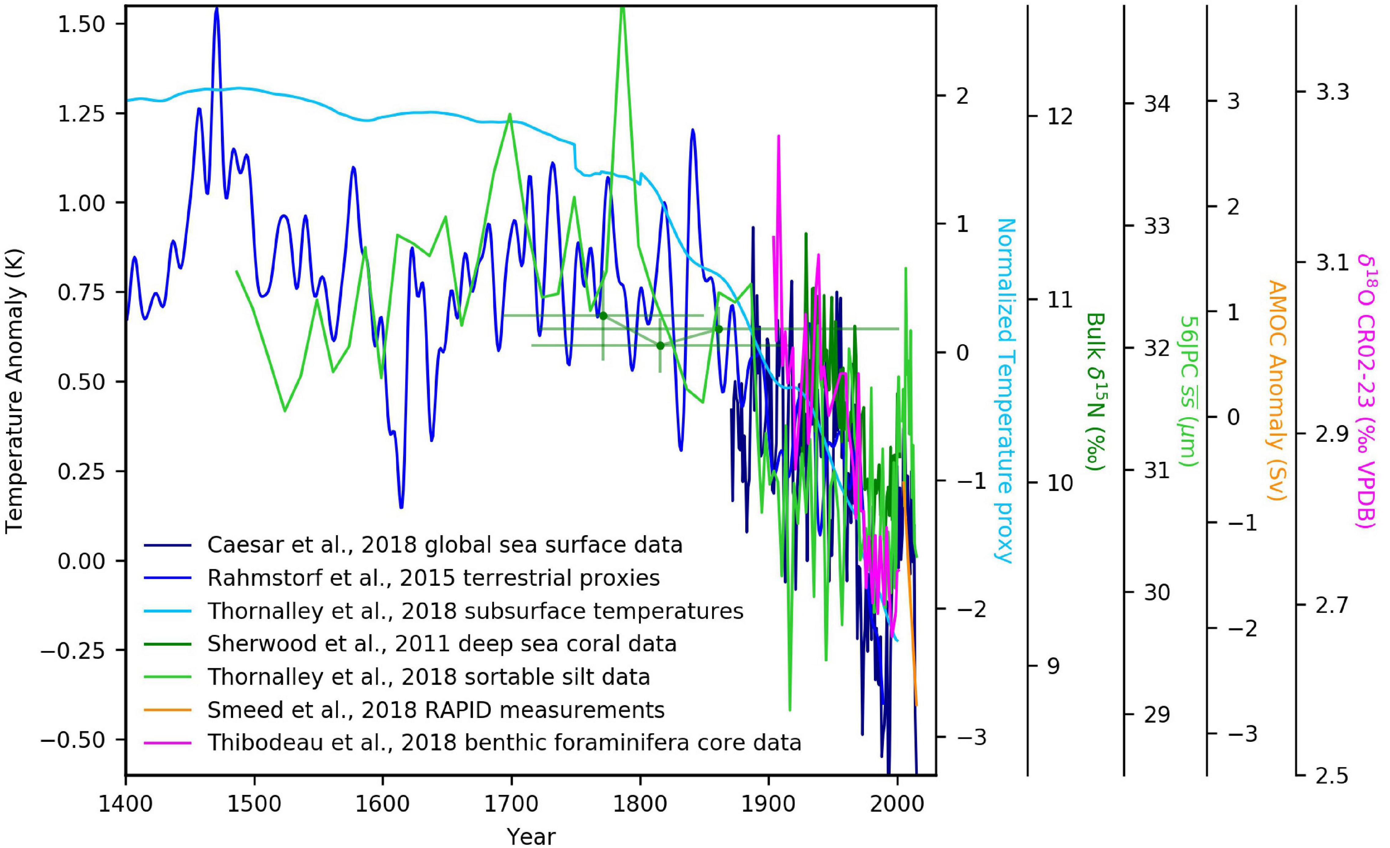
Figure 9. Trend of the strength of the overturning circulation (AMOC) in observations since 1400 from various proxies. Shown are (i) the long-term evolution of the sea surface and land temperatures in the North Atlantic region (different shades of blue; Rahmstorf et al., 2015; Caesar et al., 2018; Thornalley et al., 2018), (ii) the long-term evolution of the ocean heat content of the Atlantic (red, Zanna et al., 2019), (iii) the long-term evolution using data from deep sea cores [light green (Thornalley et al., 2018), dark green (Sherwood et al., 2011), and magenta (Thibodeau et al., 2018)] and (iv) the linear trend of in situ AMOC monitoring by the RAPID project (orange, Smeed et al., 2018).

Currently, while these findings provide strong evidence that the Atlantic Meridional Overturning Circulation has weakened relative to preindustrial times, there is insufficient data to quantify the exact magnitude of the weakening, or to properly attribute it to anthropogenic forcing (IPCC, 2019). This is also due to the fact that the ensemble means of the latest generation of climate models (CMIP6) show no trend in the strength of the overturning circulation over the historical period (Weijer et al., 2020). However, this might be due to an overestimation of the anthropogenic aerosol forcing in a majority of the models leading to a cooling of the subpolar North Atlantic and a subsequent AMOC strengthening. This is supported by the fact that those ensemble members that capture the North Atlantic cold blob, i.e., the SST fingerprint of a weaker AMOC, show a weakening of the AMOC over the historical period (Menary et al., 2020). For the future, the simulations of all CMIP6 models respond to the increasing greenhouse gas emissions with an AMOC weakening, showing on average a decline of 24–39%, depending on the emission scenario, over the course of the twenty-first century. When using the observed strength of the AMOC by RAPID/MOCHA as a constraint the mean decline increases, in particular for the low-emission scenarios, to 34–45% (Weijer et al., 2020).

Actions for Better Climate Change Monitoring

The international ocean observing community has made persistent efforts in developing new technologies, observation networks and data sharing protocols to deliver credible climate change indicators and useful ocean information to a variety of users in a timely manner and at a global scale. Here we identify the progress of the global monitoring efforts and make some recommendations to fill some of the gaps in the coming years.

High quality and global coverage observations are essential to monitor the ocean temperature changes (Abraham et al., 2013). The primary instruments of the ocean subsurface observing system since the 1940s are MBTs, XBTs, Nansen/Niskin bottles, and CTDs (Figure 10A). MBTs typically go down to ∼125–250 m and were widely deployed from 1938 to the early 1960s. Shallow XBTs (e.g., T4/T6) reach 450 m, and were widely deployed during the 1970s∼1980s whereas deep XBTs (e.g., T7/DB) provide data to 800 m, and were widely used during the 1990s and early 2000s. The Argo Program, designed in 1998 achieved its initial goal of 3000 profiling floats in November 2007. Since 2007, the data coverage is > 80% of the global ocean area (3 by 3 degree box) from 0 to 1,200 m depth and > 70% for 1,200–2,000 m depth (Figure 10B; Meyssignac et al., 2019). Maintaining and improving the current ocean observation system are strongly recommended to ensure the accurate ocean climate monitoring. It is also essential to improve the historical record, for example, by recovering un-digitized temperature (OHC) and other observations.

FIGURE 10

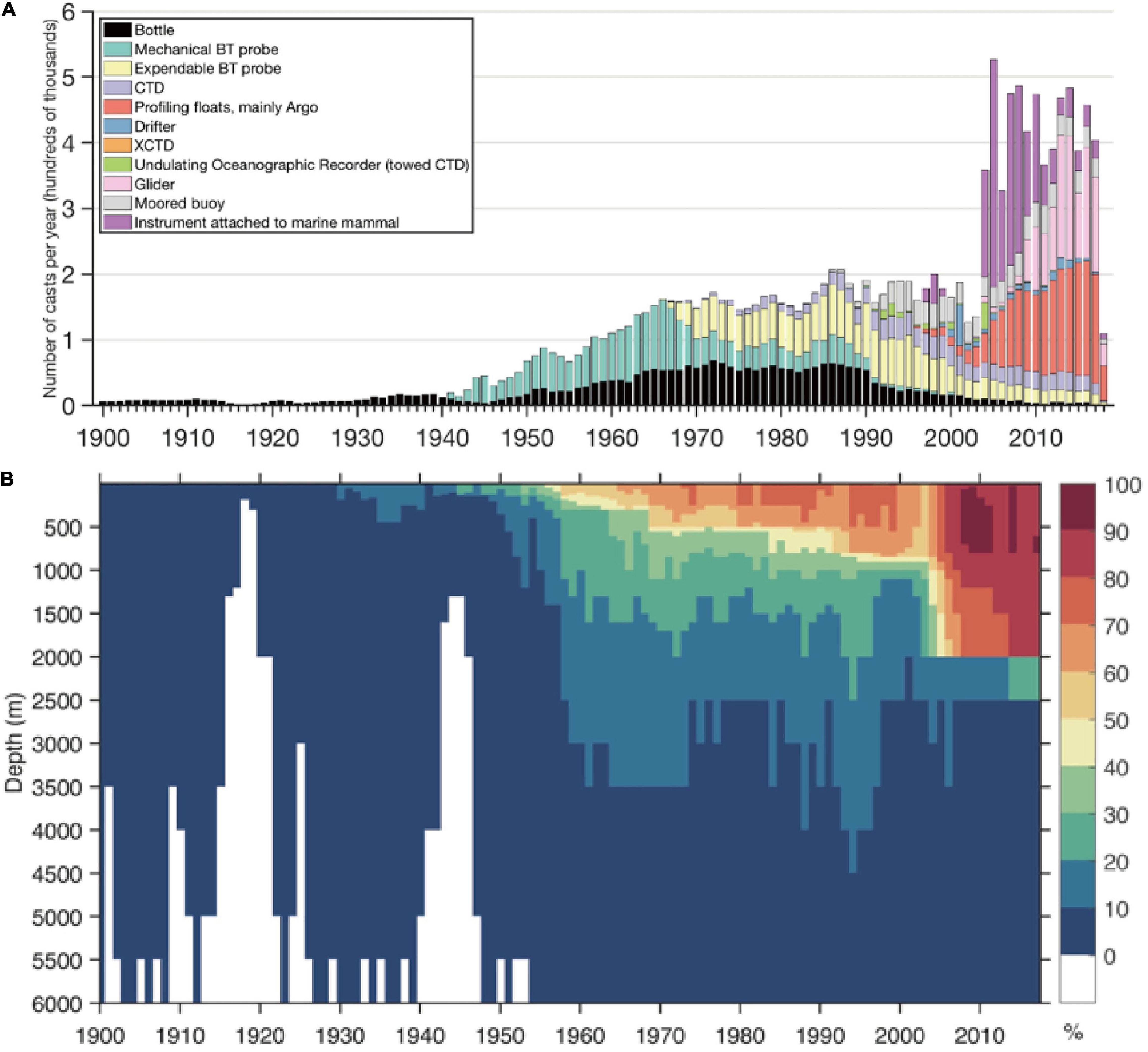
Figure 10. (A) Number of subsurface ocean temperature profiles per year by instrument type 1900–2017. (BT, Bathythermograph; CTD, Conductivity-Temperature-Depth; XCTD, Expendable CTD). (B) Ocean subsurface observation coverage. Percentage (%) of data coverage for 3 × 3 boxes over the global ocean area from 5 to 6,000 m. Figure from Meyssignac et al. (2019).

Some limitations remain for the current ocean observation network, particularly for coastal regions, marginal seas, deep ocean regions below 2,000 m. It is important to establish a deep ocean system in the future to monitor ocean changes below 2,000 m, thus to provide a complete estimate of earth’s energy imbalance (Johnson et al., 2015; von Schuckmann et al., 2016). Currently, boundary currents are not fully represented by Argo as floats can swiftly pass through the energetic regions, e.g., western boundary current (WBC) regions which could induce an inverse cascade of kinetic energy and affect the large scale low-frequency variability (Wang et al., 2017; Llovel et al., 2018). Achieving adequate sampling will require an observing system design based on a mixture of observing technologies adopted to the different operating environments. There is a need to develop/maintain multiple platform observations for cross-validation and calibration purposes (Meyssignac et al., 2019).

Intensive national and international efforts focused on carbonate chemistry monitoring, biological observations and biogeochemical/ecological forecast modeling over the past decade have shed light on the status and impacts of ocean acidification on local to global scales. International observing networks deployed around the world which use moorings, repeat hydrography research cruise transects, ships of opportunity, and fixed ocean time-series to track ocean chemistry include the Global Ocean Ship-based Hydrographic Investigations Program (GO-SHIP) surveys, the Surface Ocean CO₂ Observing Network (SOCONET), the Ship of Opportunity Program (SOOP) volunteer observing ships, and the Ocean Sustained Interdisciplinary Time-series Environment Observation System (OceanSITES) time-series stations in the Atlantic, Pacific, and Indian oceans (Figure 11). These have provided essential, climate quality carbonate chemistry observations needed to understand ocean acidification in open waters. Biogeochemical Argo platforms, still under development, will increase the availability of pH profiles throughout the water column, along with other hydrographic parameters. In an effort to both coordinate with these international efforts and to coordinate with and expand national ocean acidification observing efforts, the Global Ocean Acidification Observing Network (GOA-ON) was launched in 2013. Through GOA-ON, organizations and scientists have established observation standards, enhanced data sharing, and quantified global and regional ocean acidification trends to identify areas of heightened vulnerability or resilience.

FIGURE 11

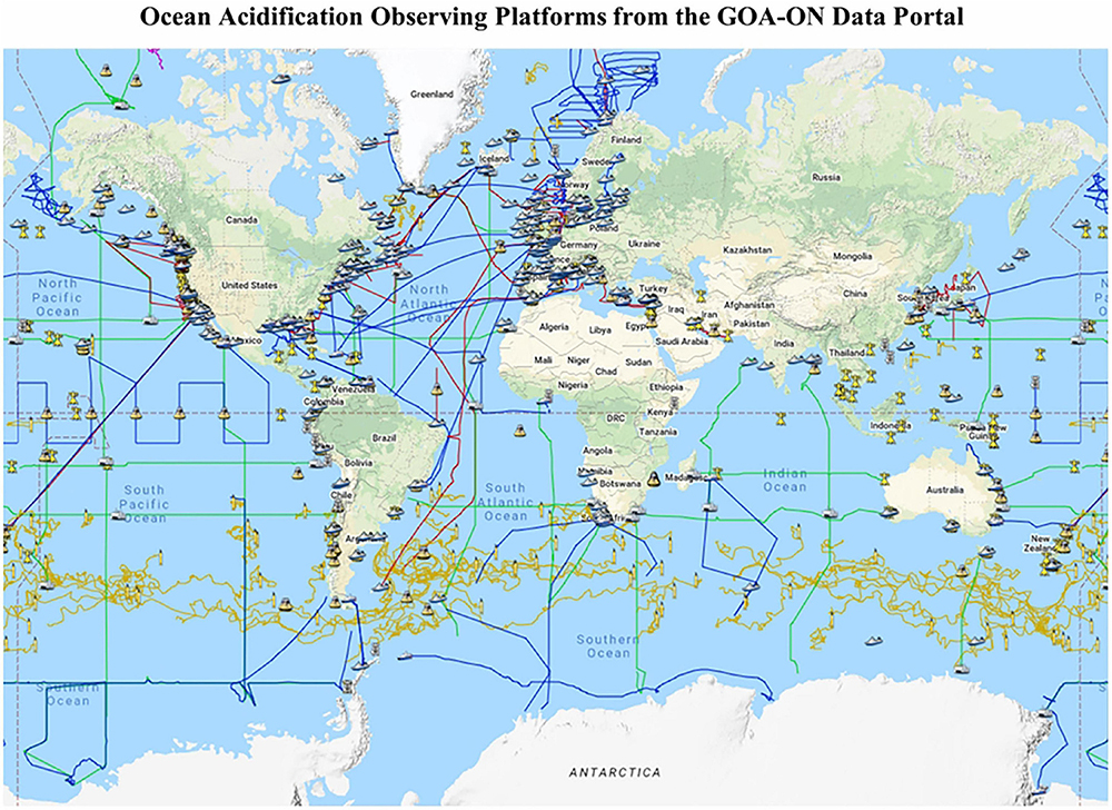
Figure 11. Visualization of ocean acidification data and data synthesis products being collected around the world from a wide range of sources, including moorings, research cruises, and fixed time series stations. Figure source GOA-ON Data Portal (http://portal.goa-on.org/).

There have been many significant leaps in comprehending global ocean acidification trends and impacts and more research is needed to better inform models and improve predictions of the Earth system response to ocean acidification (Jewett et al., 2020). This includes the relationship between the impacts of ocean acidification and other stressors, such as warming, on organisms and communities. Understanding the direct and indirect impacts on marine populations and communities and the capacity of organisms to acclimate or adapt to the changes in ocean acidification-induced ocean chemistry will be extremely important in determining and predicting the economic, ecological, and societal impacts of ocean acidification. There remains a strong need for more extensive monitoring in coastal regions, including access to high quality, low-cost sensors to do this monitoring, and to satellite data and research into the long-term trends in ocean chemistry beyond the observational record (paleo-OA).

While dissolved oxygen data coverage has been proven to be sufficient to derive large scale and global trends, significant better long-term measurements are needed to address current questions. Measurements at greater spatial and temporal extent are needed in many regions in order to capture for example the high variability in oxygen content in coastal areas. In this context it is of significant importance that a variety of biogeochemical parameters are increasingly added to the automated monitoring of the global ocean, since they serve as vital indicators for changes in the biogeochemical dynamics, which cannot be analyzed detached from changes in small- and large-scale ocean dynamics.

The International Arctic Buoy Programme (IABP)⁶ maintains the fundamental Arctic Observing Network of drifting buoys which monitor ocean and sea ice circulation, as well as sea level pressure and surface temperature. While the IABP has been able to improve and maintain a denser network of drifting buoys, the prevailing winds and ocean circulation quickly carries these buoys away from the Eurasian coast of the Arctic Ocean, thus creating a recurring gap in the network during the winter that needs to be replenished since these gaps in the network hamper our ability to completely monitor and understand Arctic change (Thoman et al., 2020).

The best estimates of the long-term trends in Arctic sea ice volume are provided by models (e.g., Schweiger et al., 2019) given the paucity of in situ, pan-Arctic measurements of sea ice thickness. These models are compared to satellite retrievals of ice thickness and in situ measurements from field programs on the ice, aerial surveys (e.g., Haas et al., 2017), and submarine transits under the ice (e.g., Rothrock et al., 1999). The satellite retrievals are also compared to in situ measurements of ice thickness, and it has been shown that the primary source of uncertainty in these retrievals is the assumed depth of snow on top of the sea ice (Kwok and Cunningham, 2015; Kwok, 2018). Recently, the Multidisciplinary drifting Observatory for the Study of Arctic Climate (MOSAiC) Expedition completed a year-long drift across the Arctic Ocean (Shupe et al., 2020), and collected myriad of observations including measurements required to improve our understanding of Arctic climate processes, such as in situ measurements of snow and ice thickness, aerial and under ice surveys. Similar campaigns should be conducted routinely on a pan-Arctic scale (Haas et al., 2017; IPCC, 2019).

There are different programs dedicated to monitoring the different contributing factors of sea level change. The Argo program, mentioned before, is devoted to the monitoring of the temperature, salinity, currents and bio-optical properties of the global ocean reaching 2,000 m depths. From these globally distributed floats, changes in the density of the water column are estimated. These observations allow monitoring the contribution of the steric change of the GMSL of the ocean. With regard to the barystatic component, the GRACE space gravimetry mission (covering the period 2002–2017) and the subsequent GRACE Follow-On (from 2018 on) satellite mission are registering global anomalies of the Earth’s gravity field. To give continuity to the altimetry sea level record, Copernicus Sentinel-6 Michael Freilich satellite has been recently launched and has provided some first promising results. The launch of its twin, Sentinel 6B, is planned for 2025 (follow on of the Jason satellites). In the future the SWOT satellite will contribute to the improvement of the coastal data, due to its higher spatial resolution and in addition, this will measure river discharges and as such will be a valuable source of sea level budget from terrestrial contribution.

It is worth mentioning that when the footprint of the altimeter covers not only the sea but also the land the returning echoes are contaminated and consequently, it is not accurate enough at around 20–50 km from the coast. For retrieving altimetry data in those areas, the coastal altimetry community has investigated how to re-process these data by using different waveform retracking algorithms and applying different geophysical corrections (Vignudelli et al., 2019) and have provided different coastal altimetry databases (Birol et al., 2017; Cipollini et al., 2017; The Climate Change Initiative Coastal Sea Level Team, 2020) with more accurate data comparing to the conventional altimetry databases.

Information about the ocean circulation and its changes can be inferred from either direct measurements, proxies, model simulations and satellites. The main uncertainties regarding the trends in ocean circulation arise from the short time spans of the direct continuous measurements, the incompleteness when representing a circulation through proxies and the inherent uncertainties of the models. It is therefore essential that the existing observation programs like the Global Drifter Program (Dohan et al., 2010) and the Argo Program are sustained. This includes but is not limited to the main programs observing the AMOC, i.e., the RAPID programs (e.g., Smeed et al., 2014, 2018) that continuously measure the AMOC strength since 2004 at roughly 26°N, the SAMOC programs that measure AMOC strength in the South Atlantic and include the SAMBA array at about 34.5°S (Meinen et al., 2018; Kersale et al., 2020) and the OSNAP program (Lozier et al., 2017) measuring the overturning that feeds the AMOC since 2014.

A Visual Summary of Ocean Climate Change Indicators

International data programs like Copernicus and others can play a relevant role to integrate the different data sets and provide the signs for ocean climate change. With that objective Figures 12, 13 present here a final visual summary of key ocean climate change indicators and current trends based on the individual analyses of the Copernicus Marine Services (CMS), that emphasizes recent changes (1993–2019/20).

FIGURE 12

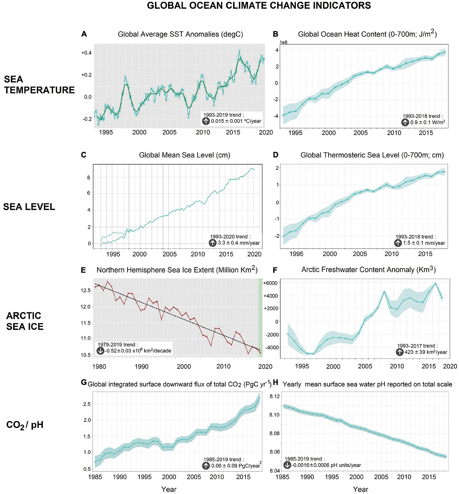
Figure 12. Visual Summary of Global Ocean Climate Change Indicators (A) Global Sea Surface Temperature (SST) anomalies (°C) during the period January 1993–December 2019. The anomalies are relative to the climatological period 1993–2014. Blue crosses (monthly mean values) and green thick line (filtered values). (B) Global Ocean Heat Content (OHC; 0–700 m; J/m²) for the period January 1993–December 2018. 60°N–60°S. Spread indicated with shade. (C) Global Mean Sea Level (cm) during the period January 1993–October 2019. Daily altimetric measurements. The time-series are low-pass filtered, the annual and semi-annual periodic signals adjusted and the curve corrected for the Glacial Isostatic Adjustment (GIA; Peltier, 2004). The dashed line indicates an estimate of the global mean sea level corrected for the drift of the TOPEX-A instrument during 1993–1998 (Ablain et al., 2017). (D) Global thermosteric sea level (0–700 m; cm) for the period January 1993–December 2018. (E) Northern Hemisphere sea ice extent (millions of Km²) during the period January 1979–December 2019 (40 years). Based on satellite passive microwave data (SMMR, SSM/I, SSMIS). Sea Ice Extent is defined as the area covered by sea ice, or area having more than 15% sea ice concentration. All northern hemisphere sea ice is included, except for lake or river ice. (F) Arctic ocean freshwater content annual anomalies (Km³) during the years 1993–2017. The regional domain is the Arctic Ocean basin with a depth > 500 m. (G) Global area integrated annual surface downward flux of total CO₂ (PgC/year) during the period January 1985–December 2019. (H) Annual global mean surface sea water pH over the period January 1985–December 2019 using a reconstruction methodology. Individual figures credited to EU Copernicus Marine Service (CMS).

FIGURE 13

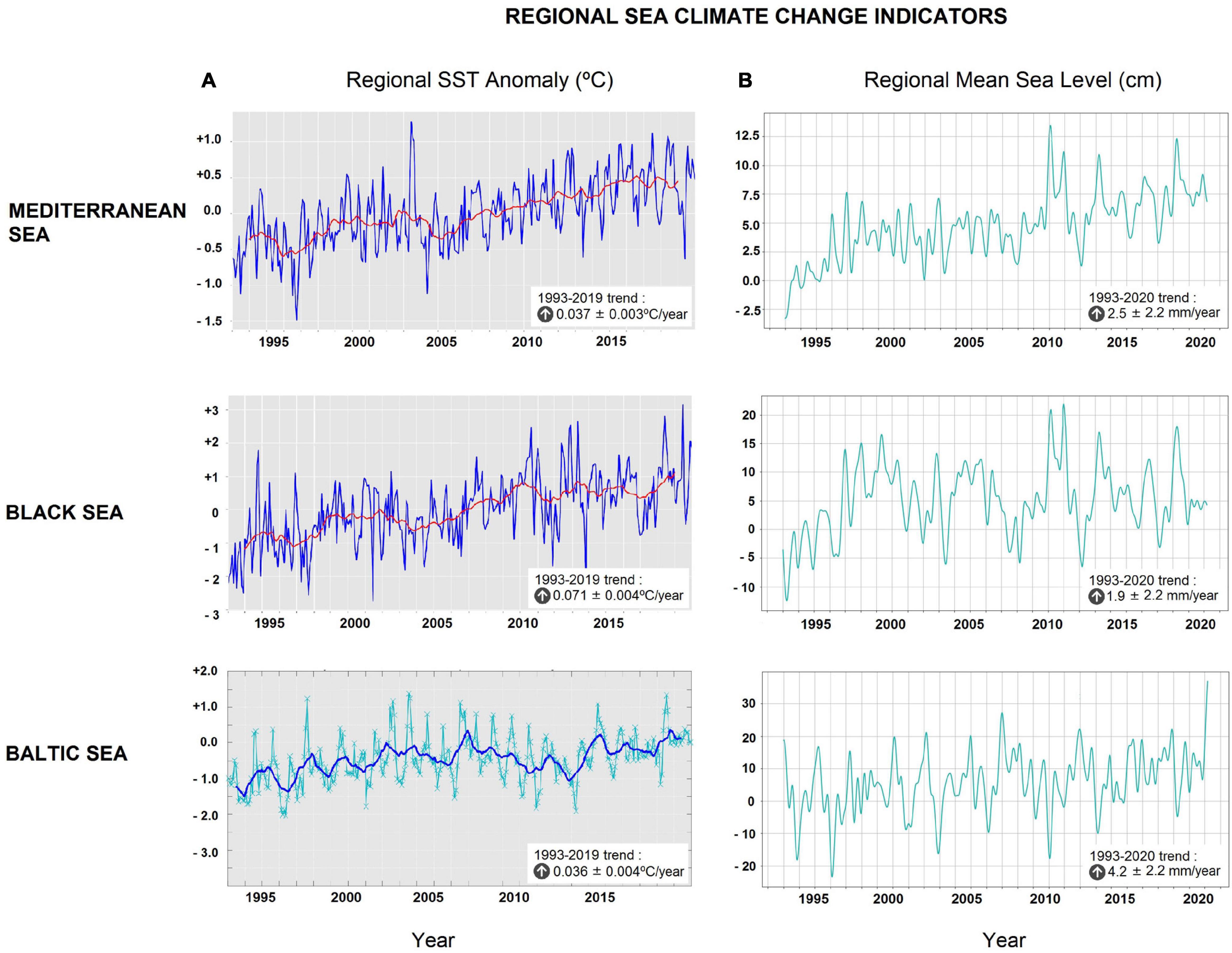
Figure 13. (A) Time series of regional Sea Surface Temperature (SST) anomalies (°C) during the period January 1993–December 2019 (27 years) in the Mediterranean Sea, the Black Sea and the Baltic Sea. Mediterranean and Black Sea: blue line (monthly mean) and red line (24-month filtered). Baltic Sea: green crosses (monthly mean) and blue line (1 year trends). The anomalies are relative to the climatological period 1993–2014. (B) Time series of regional daily Sea Level (cm) during the period January 1993–February 2020 (27 years) in the Mediterranean Sea, the Black Sea and the Baltic Sea. Altimetric data derived from the average of gridded sea level maps weighted by the cosine of the latitude. The time-series are low-pass filtered, the annual and semi-annual periodic signals adjusted, and the curve corrected for the Glacial Isostatic Adjustment (GIA; Peltier, 2004). Individual figures credited to EU Copernicus Marine Service (CMS).

Global Trends (1993–2019/20)

• According CMS, during the period 1993–2019 the global sea surface temperature (SST; Figure 12A) has increased at a mean rate of 0.15°C (±0.01°C) per decade, an increase of ∼0.4°C in 27 years. The upper (0–700 m) near-global ocean (60°N-60°S) heat content (Figure 12B) shows during that period a warming rate of 0.9 ± 0.01 Wm^–2.

• During the years 1993–2019, the global mean sea level (Figure 12C) has been rising at a mean rate of 3.3 mm year^–1 with an uncertainty of ± 0.4 mm year^–1. This represents a sea level rise of 9 cm in the 27 year period. The upper (0–700 m) near-global ocean (60°N-60°S) thermosteric sea level (the sea level resulting of the volume expansion due only to the temperature increase; Figure 12D) has risen gradually at a rate of 1.5 ± 0.1 mm year^–1, which accounts for 45% of the global mean sea level increase.

• Since 1979 the Northern Hemisphere Sea ice extent (Figure 12E) has decreased at a mean rate of −0.52 million Km² per decade (1979–2017), and accordingly the freshwater of the Arctic Ocean (Figure 12F) has increased in volume by 4,230 ± 390 Km³ per decade (data since 1993).

• The annual downward flux of CO₂ (Figure 12G) represents the ocean uptake of CO₂ over the whole ocean and has increased at a rate of 0.06 PgC year^–2 during the period 1985–2019. The annual global ocean CO₂ sink during the recent years 2017 and 2018 was, according CMS, 2.51 ± 0.17 and 2.61 ± 0.20 PgC year^–1 and the average sink over the full period (1985–2019) was 1.51 ± 0.14 PgC year^–1. The increasing concentrations of CO₂ in the ocean resulted in the ocean pH (Figure 12H) decreasing linearly at a mean rate of −0.0016 ± 0.0006 pH units per year (1985–2019) or a decrease of 0.056 pH units during the last 35 years.

Mediterranean Sea, Black Sea and Baltic Sea Trends (1993–2019/20)

CMS also provides regional analyses and we present here in Figure 13 the results for three European semi-enclosed Seas: the Mediterranean Sea, the Black Sea and the Baltic Sea.

• The sea surface temperature (SST) during the period 1993–2019 has increased at a mean rate of 0.37 ± 0.03°C per decade in the Mediterranean Sea, 0.71 ± 0.04°C per decade in the Black Sea and 0.28 ± 0.03°C per decade in the Baltic Sea, though superimposed on these trends is a strong year-to-year variability. The sea surface temperature during this period (1993–2019; 27 years) has increased, respectively, at about 1°C (Mediterranean Sea), 1.9°C (Black Sea), and 0.7/0.8°C (Baltic Sea).

• The regional mean sea level has risen during the years 1993–2020 at a rate of 2.5 mm year^–1 in the Mediterranean Sea, 1.9 mm year^–1 in the Black Sea and 4.2 mm year^–1 in the Baltic Sea. This regional indicator also presents a high interannual variability (and possibly longer-term natural variability; Garcia-Soto et al., 2012) that impacts the trend with an uncertainty of ± 2.2 mm year^–1 in the three semi-enclosed seas.

The Ocean Climate Change Indicators can be finally contextualized in larger international frameworks including the Sustainable Development Goals 13 (Climate Action) and 14 (Life Below Water) of UN Agenda 2030. Sea Surface Temperature (SST) is one of the essential climate variables (ECV) of the Global Climate Observing System (GCOS; Bojinski et al., 2014) and gives information about the flow of heat in the ocean and about modes of ocean and atmospheric variability (e.g., ENSO). Ocean Heat content is also an essential climate variable (ECV) and one of the 6 global climate indicators initially proposed by the World Meteorological Organization (WMO; Williams and Egglestob, 2017) for the Sustainable Development Goal 13 “Climate Action” (SDG13_WMO). Ocean Heat content variations produce changes in stratification and currents, impact sea ice, ice shelves and marine ecosystems, and play a role in sea level change and in the ocean-atmosphere interactions (WCRP, 2018; IPCC, 2019; von Schuckmann et al., 2020). Mean Sea Level (also an ECV) was proposed by WMO as an additional SDG-13 indicator (SDG13_WMO). It reflects the amount of heat added to the sea and the mass loss due to land ice melt, and has a direct impact on the coastal areas and population (e.g., WCRP, 2018; IPCC, 2019). Variations of sea ice cover (also ECV and SDG13_WMO indicators) can modify the key role played by the cold poles in the Earth climate, and variations in the volume of Arctic freshwater can produce changes in ocean stratification, and influence the circulation and heat transport. As part of the Global Carbon Budget (Le Quéré et al., 2018) the ocean CO₂ storage (also ECV and SDG13_WMO indicators) is evaluated every year. The ocean has absorbed about 25% of all anthropogenic CO₂ emissions since 1950 (Friedlingstein et al., 2020). A direct consequence of the uptake of carbon dioxide by the ocean is the decrease of surface ocean pH. Monitoring the surface ocean pH has become the focus of contributes to the Sustainable Development Goal 14 (SDG14) “Life below water.”

The Global Climate Observing System (GCOS) and the UN Sustainable Development Goals 13 and 14 are setting in this way the set of key ocean indicators that ensure monitoring of the climate change signals in the global ocean in an integrated and coordinated manner. And these updated climate change indicators, as the ones presented here, highlighting the impacts in the present and future ocean, will allow a better action-taking towards an urgently needed mitigation and adaptation.

Author Contributions

CG-S conceived and led the manuscript. All authors contributed to the writing of the manuscript.

Funding

This study was supported by the project of the European Union BLUEMED (GA 727453). LCh was supported by the National Natural Science Foundation of China (No. 42076202). LCa was funded by the A4 project. A4 (Grant-Aid Agreement No. PBA/CC/18/01) was carried out with the support of the Marine Institute under the Marine Research Programme funded by the Irish Government.

Conflict of Interest

The authors declare that the research was conducted in the absence of any commercial or financial relationships that could be construed as a potential conflict of interest.

Publisher’s Note

All claims expressed in this article are solely those of the authors and do not necessarily represent those of their affiliated organizations, or those of the publisher, the editors and the reviewers. Any product that may be evaluated in this article, or claim that may be made by its manufacturer, is not guaranteed or endorsed by the publisher.

Acknowledgments

Most of the authors are members of the writing team of Chapter 5 of the United Nations World Ocean Assessment II “Trends in the physical and chemical state of the ocean.” We thank the assistant editor SV and two reviewers for their helpful suggestions.

Footnotes

1. ^ COBE (Centennial in situ Observation-Based Estimates of sea surface temperature).
2. ^ HadlSST (Hadley Centre Sea Surface Temperature).
3. ^ ERSST (Extended Reconstructed Sea Surface Temperature).
4. ^ GMPE: [GHRSST (Group for High Resolution Sea Surface Temperature) Multi-Product Ensemble dataset).
5. ^ http://psc.apl.uw.edu/research/projects/arctic-sea-ice-volume-anomaly/
6. ^ http://IABP.apl.uw.edu

References

Ablain, M., Jugier, R., Zawadki, L., and Taburet, N. (2017). The TOPEX-A Drift and Impacts on GMSL Time Series (poster), Ocean Surface Topography Science Team meeting. Available online at: https://meetings.aviso.altimetry.fr/fileadmin/user_upload/tx_ausyclsseminar/files/Poster_OSTST17_GMSL_Drift_TOPEX-A.pdf (access 08/04/2021).

Google Scholar

Abraham, J., Baringer, M., Bindoff, N., Boyer, T., Cheng, L. J., Church, J. A., et al. (2013). A review of global ocean temperature observations: Implications for ocean heat content estimates and climate change. Rev. Geophys. 51, 450–483. doi: 10.1002/rog.20022

CrossRef Full Text | Google Scholar

Baumann, H. (2019). Experimental assessments of marine species sensitivities to ocean acidification and co-stressors: how far have we come? Can. J. Zool. 97, 399–408. doi: 10.1139/cjz-2018-0198

PubMed Abstract | CrossRef Full Text | Google Scholar

Baumann, H., Talmage, S. C., and Gobler, C. J. (2012). Reduced early life growth and survival in a fish in direct response to increased carbon dioxide. Nat. Clim. Change 2, 38–41. doi: 10.1038/nclimate1291

CrossRef Full Text | Google Scholar

Benveniste, J., Cazenave, A., Vignudelli, S., Fenoglio-Marc, L., Shah, R., Almar, R., et al. (2019). Requirements for a Coastal Hazards Observing System. Front. Mar. Sci. 6:348. doi: 10.3389/fmars.2019.00348

CrossRef Full Text | Google Scholar

Bianchi, D., Galbraith, E. D., Carozza, D. A., Mislan, K. A. S., and Stock, C. A. (2013). Intensification of open-ocean oxygen depletion by vertically migrating animals. Nat. Geosci. 6, 545–548. doi: 10.1038/NGEO1837

CrossRef Full Text | Google Scholar

Bindoff, N., Stott, P., AchutaRao, K., Allen, M. R., Gillett, N., and Gutzler, D., et al. (eds) (2013). “Detection and attribution of climate change: from global to regional,” in Climate Change 2013: The Physical Science Basis. Contribution of Working Group I to the Fifth Assessment Report of the Intergovernmental Panel on Climate Change. Stocker, eds T. F. Stocker, D. Qin, G. K. Plattner, M. Tignor, S. K. Allen, J. Boschung, et al. (Cambridge: Cambridge University Press), 867–952.

Google Scholar

Birol, F., Fuller, N., Lyard, F., Cancet, M., Niño, F., Delebecque, C., et al. (2017). Coastal applications from nadir altimetry: example of the X-TRACK regional products. Adv. Space Res. 59, 936–953. doi: 10.1016/j.asr.2016.11.005

CrossRef Full Text | Google Scholar

Bojinski, S., Verstraete, M., Peterson, T. C., Richter, C., Simmons, A., and Zemp, M. (2014). The concept of Essential Climate Variables in support of climate research, applications, and policy. Bull Am. Meteorol. Soc. 95, 1431–1443. doi: 10.1175/BAMS-D-13-00047.1

CrossRef Full Text | Google Scholar

Boyer, T., Domingues, C., Good, S., Johnson, G. C., Lyman, J. M., Ishii, M., et al. (2016). Sensitivity of global upper-ocean heat content estimates to mapping methods, XBT bias corrections, and baseline climatologies. J. Clim. 29, 4817–4842. doi: 10.1175/JCLI-D-15-0801.1

CrossRef Full Text | Google Scholar

Breitburg, D. L., Salisbury, J., Bernhard, J. M., Cai, W. J., Dupont, S., Doney, S. C., et al. (2015). And on top of all that…Coping with ocean acidification in the midst of many stressors. Oceanogr. 28, 48–61. doi: 10.5670/oceanog.2015.31

CrossRef Full Text | Google Scholar

Bryden, H. L., Longworth, H. R., and Cunningham, S. A. (2005). Slowing of the Atlantic meridional overturning circulation at 25°N. Nature 438, 655–657. doi: 10.1038/nature04385

PubMed Abstract | CrossRef Full Text | Google Scholar

Caesar, L., McCarthy, G. D., Thornalley, D. J. R., and Rahmstorf, S. (2021). Current Atlantic Meridional Overturning Circulation weakest in last millennium. Nat. Geosci. 14, 118–120. doi: 10.1038/s41561-021-00699-z

CrossRef Full Text | Google Scholar

Caesar, L., Rahmstorf, S., Robinson, A., Feulner, G., and Saba, V. (2018). Observed fingerprint of a weakening Atlantic Ocean overturning circulation. Nature 556:191. doi: 10.1038/s41586-018-0006-5

PubMed Abstract | CrossRef Full Text | Google Scholar

Caldeira, K., and Wickett, M. E. (2003). Anthropogenic carbon and ocean pH. Nature 425:365. doi: 10.1038/425365a

PubMed Abstract | CrossRef Full Text | Google Scholar

Campbell, A. L., Levitan, D. R., Hosken, D. J., and Lewis, C. (2016). Ocean acidification changes the male fitness landscape. Sci. Rep. 6:31250. doi: 10.1038/srep31250

PubMed Abstract | CrossRef Full Text | Google Scholar

Carpenter, J. H. (1965). The accuracy of the Winkler method for dissolved oxygen analysis. Limnol. Oceanogr. 10, 135–140. doi: 10.4319/lo.1965.10.1.0135

CrossRef Full Text | Google Scholar

Cazenave, A., Hamlington, B., Horwath, M., Barletta, V. R., Benveniste, J., Chambers, D., et al. (2019). Observational requirements for long-term monitoring of the global mean sea level and its components over the altimetry era. Front. Mar. Sci. 6:582. doi: 10.3389/fmars.2019.00582

CrossRef Full Text | Google Scholar

Cheng, L., Abraham, J., Goni, G., Boyer, T., Wijfelds, S., Cowley, R., et al. (2016). XBT Science: Assessment of instrumental biases and errors. Bull. Am. Meteorol. Soc. 97, 924–933. doi: 10.1175/BAMS-D-15-00031.1

CrossRef Full Text | Google Scholar

Cheng, L., Abraham, J., Hausfather, Z., and Trenberth, K. (2019a). How fast are the oceans warming? Science 363, 128–129. doi: 10.1126/science.aav7619

PubMed Abstract | CrossRef Full Text | Google Scholar

Cheng, L., Abraham, J., Trenberth, K., Fasullo, J., Boyer, T., Locarnini, R., et al. (2021). Upper ocean temperatures hit record high in 2020. Adv. Atmos. Sci. 38, 523–530. doi: 10.1007/s00376-021-0447-x

CrossRef Full Text | Google Scholar

Cheng, L., Abraham, J., Zhu, J., Trenberth, K., Fasullo, J., Boyer, T., et al. (2020). Record-setting ocean warmth continued in 2019. Adv. Atmos. Sci. 37, 137–142. doi: 10.1007/s00376-020-9283-7

CrossRef Full Text | Google Scholar

Cheng, L., Trenberth, K., Fasullo, J., Abraham, J., Boyer, T., Von Schuckmann, K., et al. (2018a). Taking the pulse of the planet. EOS 98, 14–16. doi: 10.1029/2017EO081839

CrossRef Full Text | Google Scholar

Cheng, L., Trenberth, K., Fasullo, J., Boyer, T., Abraham, J., and Zhu, J. (2017). Improved estimates of ocean heat content from 1960 to 2015. Sci. Adv. 3:1601545. doi: 10.1126/sciadv.1601545

PubMed Abstract | CrossRef Full Text | Google Scholar

Cheng, L., Wang, G., Abraham, J., and Huang, G. (2018b). Decadal ocean heat redistribution since the late 1990s and its association with key climate modes. Climate 6:91. doi: 10.3390/cli6040091

CrossRef Full Text | Google Scholar

Cheng, L., Zhu, J., Abraham, J., Trenberth, K. E., Fasullo, J. T., Zhang, B., et al. (2019b). 2018 continues record global ocean warming. Adv. Atmos. Sci. 36, 249–252.

Google Scholar

Cipollini, P., Calafat, F. M., Jevrejeva, S., Melet, A., and Prandi, P. (2017). Monitoring sea level in the coastal zone with satellite altimetry and tide gauges. Surv. Geophys. 38, 33–57.

Google Scholar

Codispoti, L. A. (2010). Interesting times for marine N2O. Science 327, 1339–1340. doi: 10.1126/science.1184945

PubMed Abstract | CrossRef Full Text | Google Scholar

Comiso, J. C. (2017). Bootstrap Sea Ice Concentrations from Nimbus-7 SMMR and DMSP SSM/I-SSMIS, Version 3. Boulder, CO: NASA National Snow and Ice Data Center Distributed Active Archive Center, doi: 10.5067/7Q8HCCWS4I0R

CrossRef Full Text | Google Scholar

Cross, J. N., Mathis, J. T., Frey, K. E., Cosca, C. E., Danielson, S. L., Bates, N. R., et al. (2014). Annual sea-air CO2 fluxes in the Bering Sea: insights from new autumn and winter observations of a seasonally ice-covered continental shelf. J. Geophys. Res. Oceans 119, 6693–6708.

Google Scholar

Dangendorf, S., Hay, C., Calafat, F. M., Marcos, M., Piecuch, C. G., Berk, K., et al. (2019). Persistent acceleration in global sea-level rise since the 1960s. Nat. Clim. Change 9, 705–710. doi: 10.1038/s41558-019-0531-8

CrossRef Full Text | Google Scholar

Desbruyères, D., McDonagh, E., King, B., and Thierry, V. (2017). Global and full-depth ocean temperature trends during the early twenty-first century from Argo and repeat hydrography. J. Clim. 30, 1985–1997. doi: 10.1175/JCLI-D-16-0396.1

CrossRef Full Text | Google Scholar

Diaz, R. J., and Rosenberg, R. (2008). Spreading dead zones and consequences for marine ecosystems. Science 321, 926–929. doi: 10.1126/science.1156401

PubMed Abstract | CrossRef Full Text | Google Scholar

Dodd, L. F., Grabowski, J. H., Piehler, M. F., Westfield, I., and Ries, J. B. (2015). Ocean acidification impairs crab foraging behaviour. Proc. Biol. Sci. 282:20150333. doi: 10.1098/rspb.2015.0333

PubMed Abstract | CrossRef Full Text | Google Scholar

Dohan, K., Bonjean, F., Centurioni, L., Cronin, M., Lagerloef, G., Lee, D.-K., et al. (2010). “Measuring the global ocean surface circulation with satellite and in situ observations,” in Proceedings of the OceanObs’09: Sustained Ocean Observations and Information for Society, Venice, Italy, 1–25 September 2009, Vol. 2, eds J. Hall, D. E. Harrison, and D. Stammer (European Space Agency Publication WPP-306). doi: 10.5270/OceanObs09.cwp.23

CrossRef Full Text | Google Scholar

Domingues, C., Church, J., White, N., Gleckler, P., Wijffels, S., Barker, P., et al. (2008). Improved estimates of upper-ocean warming and multi-decadal sea-level rise. Nature 453:1090. doi: 10.1038/nature07080

PubMed Abstract | CrossRef Full Text | Google Scholar

Durack, P., Gleckler, P., Landerer, F., and Taylor, K. (2014). Quantifying underestimates of long-term upper-ocean warming. Nat. Clim. Chang. 4, 999–1005. doi: 10.1038/nclimate2389

CrossRef Full Text | Google Scholar

Durack, P., Wijffels, S. E., and Matear, R. J. (2012). Ocean salinities reveal strong global water cycle intensification during 1950 to 2000. Science 336:455. doi: 10.1126/science.1212222

PubMed Abstract | CrossRef Full Text | Google Scholar

England, M., McGregor, S., Spence, P., Meel, G. A., Timmermann, A., Cai, W., et al. (2014). Recent intensification of wind-driven circulation in the Pacific and the ongoing warming hiatus. Nat. Clim. Chang. 4, 222–227. doi: 10.1038/nclimate2106

CrossRef Full Text | Google Scholar

Fallah, B., Cubasch, U., Prömmel, K., and Sodoudi, S. (2016). A numerical model study on the behaviour of Asian summer monsoon and AMOC due to orographic forcing of Tibetan Plateau. Clim. Dyn. 47, 1485–1495. doi: 10.1007/s00382-015-2914-5

CrossRef Full Text | Google Scholar

Feely, R. A., Doney, S. C., and Cooley, S. R. (2009). Ocean acidification: Present conditions and future changes in a high-CO2 world. Oceanogr. 22, 36–47. doi: 10.5670/oceanog.2009.95

CrossRef Full Text | Google Scholar

Feely, R. A., Sabine, C. L., Hernandez-Ayon, J. M., Ianson, D., and Hales, B. (2008). Evidence for upwelling of corrosive “acidified” water onto the continental shelf. Science 320, 1490–1492. doi: 10.1126/science.1155676

PubMed Abstract | CrossRef Full Text | Google Scholar

Fetterer, F., Knowles, K., Meier, W. N., Savoie, M., and Windnagel, A. K. (2017). Sea Ice Index, Version 3. Boulder, CO: NSIDC: National Snow and Ice Data Center, doi: 10.7265/N5K072F8

CrossRef Full Text | Google Scholar

Fontela, M., García-Ibáñez, M. I., Hansell, D. A., Mercier, H., and Pérez, F. F. (2016). Dissolved Organic Carbon in the North Atlantic Meridional Overturning Circulation Sci. Rep. 6, 26931. doi: 10.1038/srep26931

PubMed Abstract | CrossRef Full Text | Google Scholar

Foster, G., and Abraham, J. (2015). Lack of Evidence for a Slowdown in Global Temperature, US Climate Variability and Predictability Program (CLIVAR), Vol. 13. 6–9. Available online at: https://usclivar.org/sites/default/files/documents/2015/Variations2015Summer.pdf (access: 08/04/2021).

Google Scholar

Frajka-Williams, E. (2015). Estimating the Atlantic overturning at 26 ° N using satellite altimetry and cable measurements Geophys. Res. Lett. 42, 3458–3464. doi: 10.1002/2015GL063220

CrossRef Full Text | Google Scholar

Frajka-Williams, E., Ansorge, I. J., Baehr, J., Bryden, H. L., Chidichimo, M. P., Cunningham, S. A., et al. (2019). Atlantic meridional overturning circulation: observed transport and variability. Front. Mar. Sci. 6:260. doi: 10.3389/fmars.2019.00260

CrossRef Full Text | Google Scholar

Frederikse, T., Landerer, F., Caron, L., Adhikari, S., Parkes, D., Humphrey, V. W., et al. (2020). The causes of sea-level rise since 1900. Nature 584, 393–397. doi: 10.1038/s41586-020-2591-3

PubMed Abstract | CrossRef Full Text | Google Scholar

Friedlingstein, P., O’Sullivan, M., Jones, M. W., Andrew, R. M., Hauck, J., Olsen, A., et al. (2020). Global Carbon Budget 2020. Earth Syst. Sci. Data 12, 3269–3340. doi: 10.5194/essd-12-3269-2020

CrossRef Full Text | Google Scholar

Garcia-Soto, C., Vázquez-Cuervo, J., Clemente-Colón, P., and Hernández, F. (2012). Satellite oceanography and climate change. Deep Sea Res. Part II 77-80, 1–9. doi: 10.1016/j.dsr2.2012.07.004

CrossRef Full Text | Google Scholar

Gleckler, P., Durack, P., Stouffer, R., Johnson, G., and Forest, C. (2016). Industrial-era global ocean heat uptake doubles in recent decades. Nat. Clim. Chang. 6, 394–398. doi: 10.1038/nclimate2915

CrossRef Full Text | Google Scholar

Goni, G., Sprintall, J., Bringas, F., Cheng, L., Cirano, M., Dong, S., et al. (2019). More than 50 years of successful continuous temperature section measurements by the global expendable bathythermograph Network, its integrability, societal benefits, and future. Front. Mar. Sci. 6:452. doi: 10.3389/fmars.2019.00452

CrossRef Full Text | Google Scholar

Gouretski, V., and Cheng, L. (2020). Correction for systematic errors in the global dataset of temperature profiles from mechanical bathythermographs. J. Atmos. Ocean. Tech. 37, 841–855. doi: 10.1175/JTECH-D-19-0205.1

CrossRef Full Text | Google Scholar

Gouretski, V., and Koltermann, K. (2007). How much is the ocean really warming? Geophys. Res. Lett. 34:L01610. doi: 10.1029/2006GL027834

CrossRef Full Text | Google Scholar

Gregory, J. M., Griffies, S. M., Hughes, C. W., Lowe, J. A., Church, J. A., Fukimori, I., et al. (2019). Concepts and terminology for sea level: mean, variability and change, both local and global. Surv. Geophys. 40, 1251–1289. doi: 10.1007/s10712-019-09525-z

CrossRef Full Text | Google Scholar

Gruber, N., Clement, D., Carter, B. R., Feely, R. A., Van Heuven, S., Hoppema, M., et al. (2019a). The oceanic sink for anthropogenic CO2 from 1994 to 2007. Science 363, 1193–1199. doi: 10.1126/science.aau5153

PubMed Abstract | CrossRef Full Text | Google Scholar

Gruber, N., Landschützer, P., and Lovenduski, N. S. (2019b). The variable Southern Ocean carbon sink. Annu. Rev. Mar. 11, 159–186. doi: 10.1146/annurev-marine-121916-063407

PubMed Abstract | CrossRef Full Text | Google Scholar

Haas, C., Beckers, J., King, J., Silis, A., Stroeve, J., Wilkinson, J., et al. (2017). Ice and snow thickness variability and change in the high Arctic Ocean observed by in situ measurements. Geophys. Res. Lett. 44, 10,462-10,469. doi: 10.1002/2017GL075434

CrossRef Full Text | Google Scholar

Hansen, J., Sato, M., Kharecha, P., and Von Schuckmann, K. (2011). Earth’s energy imbalance and implications. Atmos. Chem. Phys. 11, 13421–13449. doi: 10.5194/acp-11-13421-2011

CrossRef Full Text | Google Scholar

Hartmann, D., Klein Tank, A. M. G., Rusticcuci, M., Alexander, L. V., Bronnimann, S., and Raman Charabi, Y. A., et al. (eds) (2013). “Observations: atmosphere and surface,” in Climate Change 2013: The Physical Science Basis: Contribution of Working Group I to the Fifth Assessment Report of the Intergovernmental Panel on Climate Change, eds T. F. Stocker, D. Qin, G. K. Plattner, M. Tignor, S. K. Allen, J. Boschung, et al. (Cambridge: Cambridge University Press), 159–254.

Google Scholar

Helm, K. P., Bindoff, N. L., and Church, J. A. (2011). Observed decreases in oxygen content of the global ocean. Geophys. Res. Lett. 38:L23602. doi: 10.1029/2011GL049513

CrossRef Full Text | Google Scholar

Hirahara, S., Ishii, M., and Fukuda, Y. (2014). Centennial-scale sea surface temperature analysis and its uncertainty. J. Clim. 27, 57–75. doi: 10.1175/JCLI-D-12-00837.1

CrossRef Full Text | Google Scholar

Hoegh-Guldberg, O., Poloczanska, E. S., Skirving, W., and Dove, S. (2017). Coral reef ecosystems under climate change and ocean acidification. Front. Mar. Sci. 4:158. doi: 10.3389/fmars.2017.00158

CrossRef Full Text | Google Scholar

Hönisch, B., Ridgwell, A., Schmidt, D. N., Thomas, E., Gibbs, S. J., Sluijs, A., et al. (2012). The geological record of ocean acidification. Science 335, 1058–1063. doi: 10.1126/science.1208277

PubMed Abstract | CrossRef Full Text | Google Scholar

Hu, S. and Fedorov, A. (2017). The extreme El Niño of 2015-2016 and the end of global warming hiatus. Geophys. Res. Lett. 44, 3816–3824. doi: 10.1002/2017GL072908

CrossRef Full Text | Google Scholar

Huang, B., Thorne, P., Banzon, V., Boyer, T., Chepurin, G., Lawrimore, J. H., et al. (2017). Extended reconstructed sea surface temperature, version 5 (ERSSTv5): upgrades, validations, and intercomparisons. J. Clim. 30, 8179–8205. doi: 10.1175/JCLI-D-16-0836.1

CrossRef Full Text | Google Scholar

IPCC (2019). IPCC Special Report on the Ocean and Cryosphere in a Changing Climate, eds D. H. O. Pörtner, D. C. Roberts, V., Masson-Delmotte, P. Zhai, M. Tignor, E. Poloczanska, et al. (Geneva: IPCC).

Google Scholar

Ishii, M., Fukuda, Y., Hirahara, S., Yasui, S., Suzuki, T., and Sato, K. (2017). Accuracy of global upper ocean heat content estimation expected from present observational data sets. Sola 13, 163–167. doi: 10.2151/sola.2017-030

PubMed Abstract | CrossRef Full Text | Google Scholar

Ishii, M., Shouji, A., Sugimoto, S., and Matsumoto, T. (2005). Objective analyses of sea-surface temperature and marine meteorological variables for the 20th century using ICOADS and the Kobe collection. Int. J. Climatol. 25, 865–879. doi: 10.1002/joc.1169

CrossRef Full Text | Google Scholar

Ito, T., Minobe, S., Long, M. C., and Curtis, D. (2017). Upper ocean O2 trends: 1958–2015. Geophys. Res. Lett. 44, 4214–4223. doi: 10.1002/2017GL073613

CrossRef Full Text | Google Scholar

Jackson, L. C., Peterson, K. A., Robert, C. D., and Wood, R. A. (2016). Recent slowing of Atlantic overturning circulation as a recovery from earlier strengthening. Nat. Geosci. 9, 518–522. doi: 10.1038/ngeo2715

CrossRef Full Text | Google Scholar

Jewett, E., Osborne, E. B., Arzayus, K. M., Osgood, K., DeAngelo, B. J., and Mintz, JM, Eds (2020). NOAA Ocean, Coastal, and Great Lakes Acidification Research Plan: 2020-2029. Washington DC: NOAA.

Google Scholar

Jewett, L., and Romanou, A. (2017). Ocean acidification and other ocean changes. Clim. Sci. Special Rep. 1, 364–392. doi: 10.7930/J0QV3JQB

CrossRef Full Text | Google Scholar

Jiang, L.-Q., Carter, B. R., Feely, R. A., Lauvset, S. K., and Olsen, A. (2019). Surface ocean pH and buffer capacity: past, present and future. Sci. Rep. 9:18624. doi: 10.1038/s41598-019-55039-4

PubMed Abstract | CrossRef Full Text | Google Scholar

Johnson, G., Lyman, J., Boyer, T., Cheng, L., Domingues, C., Gilson, J., et al. (2018). Ocean heat content [in State of the Climate in 2017]. B. Am. Meteorol. Soc. 99, S72–S77. doi: 10.1175/2018BAMSStateoftheClimate.1

CrossRef Full Text | Google Scholar

Johnson, G., Lyman, J., and Purkey, S. (2015). Informing deep Argo array design using Argo and full-depth hydrographic section data. J. Atmos. Ocean. Technol. 32, 2187–2198. doi: 10.1175/JTECH-D-15-0139.1

CrossRef Full Text | Google Scholar

Kanzow, T., Cunningham, S. A., Johns, W. E., Hirschi, J. J. M., Marotzke, J., Baringer, M. O., et al. (2010). Seasonal variability of the atlantic meridional overturning circulation at 26.5°N. J. Clim. 23, 5678–5698. doi: 10.1175/2010JCLI3389.1

CrossRef Full Text | Google Scholar

Keeling, R. F., and Garcia, H. R. (2002). The change in oceanic O2 inventory associated with recent global warming. Proc. Natl. Acad. Sci. U.S.A. 99, 7848–7853. doi: 10.1073/pnas.122154899

PubMed Abstract | CrossRef Full Text | Google Scholar

Keeling, R. F., Koertzinger, A., and Gruber, N. (2010). Ocean deoxygenation in a warming world. Annu. Rev. Mar. Sci. 2, 199–229. doi: 10.1146/annurev.marine.010908.163855

PubMed Abstract | CrossRef Full Text | Google Scholar

Kersale, M., Meinen, C. S., Perez, R. C., Le Henaff, M., Valla, D., and Lamont, T. (2020). Highly variable upper and abyssal overturning cells in the South Atlantic. Sci. Adv. 6:eaba7573. doi: 10.1126/sciadv.aba7573

PubMed Abstract | CrossRef Full Text | Google Scholar

Knapp, G. P., Stalcup, M. C., and Stanley, R. J. (1991). Iodine losses during Winkler titrations. Deep Sea Res. Part I. 38, 121–128. doi: 10.1016/0198-0149(91)90057-M

CrossRef Full Text | Google Scholar

Kosaka, Y., and Xie, S. (2013). Recent global-warming hiatus tied to equatorial Pacific surface cooling. Nature 501:403. doi: 10.1038/nature12534

PubMed Abstract | CrossRef Full Text | Google Scholar

Kwiatkowski, L., Torres, O., Bopp, O., Aumont, O., Chamberlain, M., Christian, J. R., et al. (2020). Twenty-first century ocean warming, acidification, deoxygenation, and upper-ocean nutrient and primary production decline from CMIP6 model projections. Biogeosciences 17, 3439–3470. doi: 10.5194/bg-17-3439-2020

CrossRef Full Text | Google Scholar

Kwok, R. (2018). Arctic sea ice thickness, volume, and multiyear ice coverage: losses and coupled variability (1958–2018). Environ. Res. Lett. 13:105005. doi: 10.1088/1748-9326/aae3ec

CrossRef Full Text | Google Scholar

Kwok, R., and Cunningham, G. F. (2015). Variability of Arctic sea ice thickness and volume from CryoSat-2. Philos. Trans. R. Soc. A Math. Phys. Eng. Sci. 373:20140157. doi: 10.1098/rsta.2014.0157

PubMed Abstract | CrossRef Full Text | Google Scholar

Latif, M., Böning, C., Willebrand, J., Biastoch, A., Dengg, J., Keenlyside, N., et al. (2006). Is the thermohaline circulation changing? J. Clim. 19, 4631–4637. doi: 10.1175/JCLI3876.1

CrossRef Full Text | Google Scholar

Le Quéré, C., Andrew, R. M., Canadell, J. G., Stich, S., Korsvakken, J. I., Petews, G. P., et al. (2016). Global carbon budget 2016. Earth Syst. Sci. Data 8, 605–649. doi: 10.5194/essd-8-605-2016

CrossRef Full Text | Google Scholar

Le Quéré, C., Andrew, R. M., Friedlingstein, P., Sitch, S., Julia Pongratz, J., Manning, A. C., et al. (2018). Global Carbon Budget 2017. Earth Syst. Sci. Data 10, 405–448. doi: 10.5194/essd-10-405-2018

CrossRef Full Text | Google Scholar

Lemasson, A. J., Fletcher, S., Hall-Spencer, J. M., and Knights, A. M. (2017). Linking the biological impacts of ocean acidification on oysters to changes in ecosystem services: a review. J. Exp. Mar. Biol. Ecol. 492, 49–62. doi: 10.1016/j.jembe.2017.01.019

CrossRef Full Text | Google Scholar

Levitus, S., Antonov, J. I., Boyer, T. P., Baranova, O. K., Garcia, E., Locarnini, R. A., et al. (2012). World ocean heat content and thermosteric sea level change (0-2000 m), 1955-2010. Geophys. Res. Lett. 39:10. doi: 10.1029/2012GL051106

CrossRef Full Text | Google Scholar

Levitus, S., Antonov, J. I., Boyer, T. P., and Stephens, C. (2000). Warming of the world ocean. Science 287, 2225–2229. doi: 10.1126/science.287.5461.2225

CrossRef Full Text | Google Scholar

Li, F., Lozier, M. S., and Johns, W. (2017). Calculating the meridional volume, heat and freshwater transports from an observing system in the subpolar North Atlantic: observing system simulation experiment. J. Atmos. Ocean. Tech. 34, 1483–1500. doi: 10.1175/JTECH-D-16-0247.1

CrossRef Full Text | Google Scholar

Llovel, W., Penduff, T., Meyssignac, B., Molines, J.-M., Terray, L., Bessières, L., et al. (2018). Contributions of Atmospheric Forcing and Chaotic Ocean Variability to Regional Sea Level Trends Over 1993–2015. Geophys. Res. Lett. 45, 405–413. doi: 10.1029/2018GL080838

CrossRef Full Text | Google Scholar

Longworth, H. R., Bryden, H. L., and Baringer, M. O. (2011). Historical variability in Atlantic meridional baroclinic transport at 26.5°N from boundary dynamic height observations Deep-Sea Res. Part II 58, 1754–1767. doi: 10.1016/j.dsr2.2010.10.057

CrossRef Full Text | Google Scholar

Lozier, M. S., Bacon, S., Bower, A., Cunningham, S. A., de Jong, M. F., de Steur, L., et al. (2017). Overturning in the subpolar north atlantic program: a new international ocean observing system. Bull. Amer. Meteor. 98, 737–752. doi: 10.1175/BAMS-D-16-0057.1

CrossRef Full Text | Google Scholar

Lyman, J. M., and Johnson, G. C. (2013). Estimating global ocean heat content changes in the upper 1800m since 1950 and the influence of climatology choice. J. Clim. 27, 1945–1957. doi: 10.1175/JCLI-D-12-00752.1

CrossRef Full Text | Google Scholar

Manabe, S., and Stouffer, R. J. (1980). Sensitivity of a global climate model to an increase of CO2 concentration in the atmosphere. J. Geophys. Res. 85, 5529–5554. doi: 10.1029/JC085iC10p05529

CrossRef Full Text | Google Scholar

Meehl, G. A., Arblaster, J. M., Fasullo, J. T., Hu, A. X., and Trenberth, K. E. (2011). Model-based evidence of deep-ocean heat uptake during surface-temperature hiatus periods. Nat. Clim. Chang. 1, 360–364. doi: 10.1038/nclimate1229

CrossRef Full Text | Google Scholar

Meier, W. N., Hovelsrud, G. K., Van Oort, B. E. H., Key, J. R., Kit, M., Michel, C., et al. (2014). Arctic sea ice in transformation: a review of recent observed changes and impacts on biology and human activity. Rev. Geophys. 52, 185–217.

Google Scholar

Meinen, C. S., Speich, S., Piola, A. R., Ansorge, I., Campos, E., Kersalé, M., et al. (2018). Meridional overturning circulation transport variability at 34.5°S during 2009–2017: Baroclinic and barotropic flows and the dueling influence of the boundaries. Geophys. Res. Lett. 45, 4180–4188. doi: 10.1029/2018GL077408

CrossRef Full Text | Google Scholar

Menary, M. B., Robson, J., Allan, R. P., Booth, B. B. B., Cassou, C., Gastineau, G., et al. (2020). Aerosol forced AMOC changes in CMIP6 historical simulations. Geophys. Res. Lett. 47:e2020GL088166. doi: 10.1029/2020GL088166

CrossRef Full Text | Google Scholar

Meredith, M., Cassotta, S., Derksen, C., Ekaykin, A., Hollowed, A., and Kofinas, G., et al. (eds) (2019). “Polar regions,” in IPCC Special Report on the Ocean and Cryosphere in a Changing Climate, eds D. H. O. Pörtner, D. C. Roberts, V. Masson-Delmotte, P. Zhai, M. Tignor, E. Poloczanska, et al. (Geneva: IPCC), 203–320.

Google Scholar

Meyssignac, B., Boyer, T., Zhao, Z., Hakuba, M. Z., Landerer, F. W., Stammer, D., et al. (2019). Measuring global ocean heat content to estimate the earth energy imbalance. Front. Mar. Sci. 6:432. doi: 10.3389/fmars.2019.00432

CrossRef Full Text | Google Scholar

Moat, B. I., Smeed, D. A., Frajka-Williams, E., Desbruyères, D. G., Beaulieu, C., Johns, W. E., et al. (2020). Pending recovery in the strength of the meridional overturning circulation at 26°N. Ocean Sci. 16, 863–874. doi: 10.5194/os-16-863-2020

CrossRef Full Text | Google Scholar

Morison, J., Kwok, R., Dickinson, S., Andersen, R., Peralta-Ferriz, C., and Morison, D. I., et al. (2021). The cyclonics mode of arctic ocean circulation. J. Phys. Ocean 51:4. doi: 10.1175/JPO-D-20-0190.1

CrossRef Full Text | Google Scholar

Morison, J., Kwok, R., Peralta-Ferriz, C., Alkire, M., Rigor, I., Andersen, R., et al. (2012). Changing Arctic ocean freshwater pathways. Nature 481, 66–70. doi: 10.1038/nature10705

PubMed Abstract | CrossRef Full Text | Google Scholar

Mulitza, S., Prange, M., Stuut, J. B., Zabel, M., Von Dobeneck, T., Itambi, A. C., et al. (2008). Sahel megadroughts triggered by glacial slowdowns of Atlantic meridional overturning. Paleoceanography 23:A4206. doi: 10.1029/2008PA001637

CrossRef Full Text | Google Scholar

Nerem, R. S., Beckley, B. D., Fasullo, J. T., Hamlington, B. D., Masters, D., and Mitchum, G. T. (2018). Climate-change–driven accelerated sea-level rise. Proc. Natl. Acad. Sci. U.S.A. 115, 2022–2025. doi: 10.1073/pnas.1717312115

PubMed Abstract | CrossRef Full Text | Google Scholar

Oppenheimer, M., Glavovic, B. C., Hinkel, J., van de Wal, R., Magnan, A. K., and Abd-Elgawad, A., et al. (eds) (2019). “Sea level rise and implications for low lying islands, coasts and communities,” in IPCC Special Report on the Ocean and Cryosphere in a Changing Climate, eds D. H. O. Pörtner, D. C. Roberts, V. Masson-Delmotte, P. Zhai, M. Tignor, E. Poloczanska, et al. (Geneva: IPCC), 321–446.

Google Scholar

Orr, J. C., Fabry, V. J., Aumont, O., Bopp, L., Doney, S. C., Feely, R. A., et al. (2005). Anthropogenic ocean acidification over the twenty-first century and its impact on calcifying organisms. Nature 437, 681–686. doi: 10.1038/nature04095

PubMed Abstract | CrossRef Full Text | Google Scholar

Oschlies, A., Brandt, P., Stramma, L., and Schmidtko, S. (2018). Drivers and mechanisms of ocean deoxygenation. Nature Geosci. 11, 467–473. doi: 10.1038/s41561-018-0152-2

CrossRef Full Text | Google Scholar

Palmer, M. D., Haines, K., Tett, S. F. B., and Ansell, T. J. (2007). Isolating the signal of ocean global warming. Geophys. Res. Lett. 34:L23610. doi: 10.1029/2007GL031712

CrossRef Full Text | Google Scholar

Peltier, R. (2004). Global glacial isostasy and the surface of the ice-age Earth: The ICE-%G (VM”) model and GRACE. Annu. Rev. Earth Planet. Sci. 32, 111–149. doi: 10.1146/annurev.earth.32.082503.144359

CrossRef Full Text | Google Scholar

Perovich, D., Meier, W., Tschudi, M., Hendricks, S., Petty, A. A., Divine, D., et al. (2020). Sea Ice. NOAA Arctic Report Card 2020, 44–53. doi: 10.25923/n170-9h57

CrossRef Full Text | Google Scholar

Polyakov, I. V., Rippeth, T. P., Fer, I., Alkire, M. B., Baumann, T. M., Carmack, E. C., et al. (2020). Weakening of cold halocline layer exposes sea ice to oceanic heat in the eastern Arctic Ocean. J. Clim. 33, 8107–8123. doi: 10.1175/JCLI-D-19-0976.1

CrossRef Full Text | Google Scholar

Rahmstorf, S., Box, J., Feulner, G., Mann, M., Robinson, A., Rutherford, S., et al. (2015). Exceptional twentieth-Century slowdown in Atlantic Ocean overturning circulation. Nat. Clim. Chang. 5, 475–480. doi: 10.1038/nclimate2554

CrossRef Full Text | Google Scholar

Rampal, P., Weiss, J., Dubois, C., and Campin, J. M. (2011). IPCC climate models do not capture arctic sea ice drift acceleration: Consequences in terms of projected sea ice thinning and decline. J. Geophys. Res. Oceans 116:C00D07. doi: 10.1029/2011JC007110

CrossRef Full Text | Google Scholar

Rayner, N., Parker, D. E., Horton, E. B., Folland, C. K., Alexander, L. V., Rowell, D. P., et al. (2003). Global analyses of sea surface temperature, sea ice, and night marine air temperature since the late nineteenth century. J. Geophys. Res. Atmos. 108:4407. doi: 10.1029/2002JD002670

CrossRef Full Text | Google Scholar

Rhein, M., Rintoul, S. R., Aoki, S., Campos, E., Chambers, D., and Feely, R. A., et al. (eds) (2013). “Observations: ocean,” in Climate Change 2013: The Physical Science Basis. Contribution of Working Group I to the Fifth Assessment Report of the Intergovernmental Panel on Climate Change, eds D. H. O. Pörtner, D. C. Roberts, V. Masson-Delmotte, P. Zhai, M. Tignor, E. Poloczanska, et al. (Cambridge: Cambridge University Press), 255–316. doi: 10.1017/CBO9781107415324.010

CrossRef Full Text | Google Scholar

Riebesell, U., Bach, L. T., Bellerby, R. G., Monsalve, J. R. B., Boxhammer, T., Czerny, J., et al. (2017). Competitive fitness of a predominant pelagic calcifier impaired by ocean acidification. Nat, Geosci. 10, 19–23. doi: 10.1038/ngeo2854

CrossRef Full Text | Google Scholar

Rigor, I. G., Colony, R. L., and Martin, S. (2000). Variations in Surface Air Temperature in the Arctic from 1979-1997. J. Clim. 13, 896–914.

Google Scholar

Rigor, I. G., and Wallace, J. M. (2004). Variations in the Age of Sea Ice and Summer Sea Ice Extent. Geophys. Res. Lett. 31:L09401. doi: 10.1029/2004GL019492

CrossRef Full Text | Google Scholar

Rigor, I. G., Wallace, J. M., and Colony, R. L. (2002). Response of sea ice to the Arctic Oscillation. J. Clim. 15, 2648–2663.

Google Scholar

Rothrock, D. A., Yu, Y., and Maykut, G. A. (1999). Thinning of Arctic sea ice. Geophys. Res. Lett. 26, 3469–3472. doi: 10.1029/1999GL010863

CrossRef Full Text | Google Scholar

Santer, B. D., Bonfils, C., Painter, J. F., Zelinka, M. D., Mears, C., Solomon, S., et al. (2014). Volcanic contribution to decadal changes in tropospheric temperature. Nat. Geosci. 7, 185–189. doi: 10.1038/ngeo2098

CrossRef Full Text | Google Scholar

Santoro, A., Buchwald, C., McLLvin, M., and Casciotti, K. L. (2011). Isotopic signature of N2O produced by marine ammonia-oxidizing archaea. Science 333, 1282–1285. doi: 10.1126/science.1208239

PubMed Abstract | CrossRef Full Text | Google Scholar

Schmidt, G. A., Shindell, D. T., and Tsigaridis, K. (2014). Reconciling warming trends. Nat. Geosci. 7, 158–160. doi: 10.1038/ngeo2105

CrossRef Full Text | Google Scholar

Schmidtko, S., Stramma, L., and Visbeck, M. (2017). Decline in global oceanic oxygen content during the past five decades. Nature 542, 335–339. doi: 10.1038/nature21399

PubMed Abstract | CrossRef Full Text | Google Scholar

Schmittner, A. (2005). Decline of the marine ecosystem caused by a reduction in the Atlantic overturning circulation. Nature 434, 628–633. doi: 10.1038/nature03476

PubMed Abstract | CrossRef Full Text | Google Scholar

Schweiger, A., Lindsay, R., Zhang, J., Steele, M., Stern, H., and Kwok, R. (2011). Uncertainty in modeled Arctic sea ice volume. J. Geophys. Res. 116:C00D06. doi: 10.1029/2011JC007084

CrossRef Full Text | Google Scholar

Schweiger, A. J., Wood, K. R., and Zhang, J. (2019). Arctic Sea Ice Volume Variability over 1901–2010: A Model-Based Reconstruction. J. Clim. 32, 4731–4752. doi: 10.1175/jcli-d-19-0008.1

CrossRef Full Text | Google Scholar

Shepherd, A., Ivins, E. R., Geruo, A., Varletta, V. R., Bentley, M. J., Bettadpur, S., et al. (2012). A reconciled estimate of ice-sheet mass balance. Science 338, 1183–1189. doi: 10.1126/science.1228102

PubMed Abstract | CrossRef Full Text | Google Scholar

Sherwood, O. A., Lehmann, M. F., Schubert, C. J., Scott, D. B., and McCarthy, M. D. (2011). Nutrient regime shift in the western North Atlantic indicated by compound-specific δ15N of deep-sea gorgonian corals. Proc. Natl. Acad. Sci. U.S.A. 108, 1011–1015. doi: 10.1073/pnas.1004904108

PubMed Abstract | CrossRef Full Text | Google Scholar

Shupe, M. D., Rex, M., Dethloff, K., Damm, E., Fong, A. A., Gradinger, R., et al. (2020). The MOSAiC Expedition: A Year Drifting with the Arctic Sea Ice. NOAA Arctic Report Card 2020. Washington DC: NOAA, doi: 10.25923/9g3v-xh92

CrossRef Full Text | Google Scholar

Slangen, A. B. A., Adloff, F., Jevrejeva, S., Leclercq, P. W., Marzeion, B., Wada, Y., et al. (2017). “A review of recent updates of sea level projections at global and regional scales,” in Integrative Study of the Mean Sea level and Its Components, eds A. Cazenave, N. Champollion, F. Paul, and J. Benveniste (New York, NY: Springer), 395–416. doi: 10.1007/978-3-319-56490-6_17

CrossRef Full Text | Google Scholar

Smeed, D. A., Josey, S. A., Beaulieu, C., Johns, W. E., Moat, B. I., Frajka-Williams, E., et al. (2018). The North Atlantic Ocean Is in a State of Reduced Overturning. Geophys. Res. Lett. 45, 1527–1533. doi: 10.1002/2017GL076350

CrossRef Full Text | Google Scholar

Smeed, D. A., McCarthy, G. D., Cunningham, S. A., Frajka-Williams, E., Rayner, D., Johns, W. E., et al. (2014). Observed decline of the Atlantic meridional overturning circulation 2004–2012. Ocean Sci. 10, 29–38. doi: 10.5194/os-10-29-2014

CrossRef Full Text | Google Scholar

Stammer, D., Cazenave, A., Ponte, R. M., and Tamisiea, M. E. (2013). Causes for contemporary regional sea level changes. Annu. Rev. Mar. Sci. 5, 21–46. doi: 10.1146/annurev-marine-121211-172406

PubMed Abstract | CrossRef Full Text | Google Scholar

Steele, M., and Boyd, T. (1998). Retreat of the cold halocline layer in the Arctic Ocean. J. Geophys. Res. 103, 10419–10435. doi: 10.1029/98JC00580

CrossRef Full Text | Google Scholar

Stendardo, I., and Gruber, N. (2012). Oxygen trends over five decades in the North Atlantic. J. Geophys. Res. Oceans 117:C11. doi: 10.1029/2012JC007909

CrossRef Full Text | Google Scholar

Stiasny, M. H., Mittermayer, F. H., Sswat, M., Voss, R., Jutfelt, F., Chierici, M., et al. (2016). Ocean acidification effects on Atlantic cod larval survival and recruitment to the fished population. PLoS ONE 11:e0155448. doi: 10.1371/journal.pone.0155448

PubMed Abstract | CrossRef Full Text | Google Scholar

Stramma, L., and Schmidtko, S. (2021). Spatial and temporal variability of oceanic oxygen changes and underlying trends. Atmos. Ocean 59, 122–132. doi: 10.1080/07055900.2021.1905601

CrossRef Full Text | Google Scholar

Sutton, A. J., Feely, R. A., Maenner-Jones, S., Musielwicz, S., Osborne, J., Dietrich, C., et al. (2019). Autonomous seawater pCO2 and pH time series from 40 surface buoys and the emergence of anthropogenic trends. Earth Syst Sci. Data 11, 421–439. doi: 10.5194/essd-11-421-2019

CrossRef Full Text | Google Scholar

Swart, N. C., Gille, S. T., Fyfe, J., and Gillet, N. P. (2018). Recent Southern Ocean warming and freshening driven by greenhouse gas emissions and ozone depletion. Nat. Geosci. 11, 836–841. doi: 10.1038/s41561-018-0226-1

CrossRef Full Text | Google Scholar

Tanhua, T., Orr, J. C., Lorenzoni, L., and Hansson, L. (2015). Theme: monitoring ocean carbon and ocean acidification. WMO Bull. 64:1.

Google Scholar

Tasoff, A. J., and Johnson, D. W. (2019). Can larvae of a marine fish adapt to ocean acidification? Evaluating the evolutionary potential of California Grunion (Leuresthes tenuis). Evol Appl. 12, 560–571. doi: 10.1111/eva.12739

PubMed Abstract | CrossRef Full Text | Google Scholar

The Climate Change Initiative Coastal Sea Level Team (2020). Coastal sea level anomalies and associated trends from Jason satellite altimetry over 2002–2018. Sci. Data 7:357. doi: 10.1038/s41597-020-00694-w

PubMed Abstract | CrossRef Full Text | Google Scholar

Thibodeau, B., Not, C., Zhu, J., Schmittner, A., Noone, D., Tabor, C., et al. (2018). Last century warming over the canadian atlantic shelves linked to weak atlantic meridional overturning circulation. Geophys. Res. Lett. 45, 12376–12385. doi: 10.1029/2018GL080083

CrossRef Full Text | Google Scholar

Thoman, R. L., Richter-Menge, J., and Druckenmiller, M. L. Eds (2020). Arctic Report Card 2020. Washington DC: NOAA, doi: 10.25923/MN5P-T549X

CrossRef Full Text | Google Scholar

Thompson, D. W., and Wallace, J. M. (1998). The Arctic oscillation signature in the wintertime geopotential height and temperature fields. Geophys. Res Lett. 25, 1297–1300. doi: 10.1029/98GL00950

CrossRef Full Text | Google Scholar

Thornalley, D. J. R., Oppo, D. W., Ortega, P., Robson, J. I., Brierley, C. M., Davis, R., et al. (2018). Anomalously weak Labrador Sea convection and Atlantic overturning during the past 150 years. Nature 556, 227–230. doi: 10.1038/s41586-018-0007-4

PubMed Abstract | CrossRef Full Text | Google Scholar

Timmermann, A., Okumura, Y., An, S. I., Clement, A., Dong, B., Guilyardi, E., et al. (2007). The influence of a weakening of the atlantic meridional overturning circulation on ENSO. J. Clim. 20, 4899–4919. doi: 10.1175/JCLI4283.1

CrossRef Full Text | Google Scholar

Trenberth, K. E., Cheng, L., Jacobs, P., Zhang, Y., and Fasullo, J. (2018). Hurricane Harvey links to ocean heat content and climate change adaptation. Earth Future 6, 730–744. doi: 10.1029/2018EF000825

CrossRef Full Text | Google Scholar

Trenberth, K. E., Fasullo, J. T., and Balmaseda, M. A. (2014). Earth’s energy imbalance. J. Clim. 27, 3129–3144. doi: 10.1175/JCLI-D-13-00294.1

CrossRef Full Text | Google Scholar

Vignudelli, S., Birol, F., Benveniste, J., Fu, L.-L., Picot, N., Raynal, M., et al. (2019). Satellite altimetry measurements of sea level in the coastal zone. Surv. Geophys. 40, 1319–1349. doi: 10.1007/s10712-019-09569-1

CrossRef Full Text | Google Scholar

von Schuckmann, K., Cheng, L., Palmer, M. D., Hansen, J., Tassone, C., Aich, V., et al. (2020). Heat stored in the Earth system: where does the energy go? Earth Syst. Sci. Data 12, 2013–2041. doi: 10.5194/essd-12-2013-2020

CrossRef Full Text | Google Scholar

von Schuckmann, K., and Le Traon, P.-Y. (2011). How well can we derive Global Ocean Indicators from Argo data? Ocean Sci. 7, 783–791. doi: 10.5194/os-7-783-2011

CrossRef Full Text | Google Scholar

von Schuckmann, K., Palmer, M. D., Trenberth, K. E., Cazenave, A., Chambers, D., Champollion, N., et al. (2016). An imperative to monitor Earth’s energy imbalance. Nat. Clim. Chang. 6, 138. doi: 10.1038/nclimate2876

CrossRef Full Text | Google Scholar

Wang, G., Cheng, L., Abraham, J., and Li, C. (2017). Consensuses and discrepancies of basin-scale ocean heat content changes in different ocean analyses. Clim. Dyn. 50, 2471–2487. doi: 10.1007/s00382-017-3751-5

CrossRef Full Text | Google Scholar

Watanabe, M., Shiogama, H., Tatebe, H., Hayashi, M., Ishii, M., and Kimoto, M. (2014). Contribution of natural decadal variability to global warming acceleration and hiatus. Nat. Clim. Chang. 4, 893–897. doi: 10.1038/nclimate2355

CrossRef Full Text | Google Scholar

WCRP (2018). Global sea-level budget 1993–present. Earth Syst. Sci. Data 10, 1551–1590. doi: 10.5194/essd-10-1551-2018

CrossRef Full Text | Google Scholar

Weijer, W., Cheng, W., Garuba, O. A., Hu, A., and Nadiga, B. T. (2020). CMIP6 Models Predict Significant 21st Century Decline of the Atlantic Meridional Overturning Circulation. Geophys. Res. Lett. 47:e2019GL086075. doi: 10.1029/2019GL086075

CrossRef Full Text | Google Scholar

Wijffels, S., Roemmich, D., Monselesan, D., Church, J., and Gilson, J. (2016). Ocean temperatures chronicle the ongoing warming of Earth. Nat. Clim. Chang. 6, 116–118. doi: 10.1038/nclimate2924

CrossRef Full Text | Google Scholar

Wilcock, R. J., Stevenson, C. D., and Roberts, C. A. (1981). An interlaboratory study of dissolved oxygen in water. Water Res. 15, 321–325. doi: 10.1016/0043-1354(81)90035-X

CrossRef Full Text | Google Scholar

Williams, M., and Egglestob, S. (2017). Using indicators to explain our changing climate to policy makers and the public. WMO Bull. 66, 33–39.

Google Scholar

Willis, J. K., Roemmich, D., and Cornuelle, B. (2004). Interannual variability in upper ocean heat content, temperature, and thermosteric expansion on global scales. J. Geophys. Res. 109:C12036. doi: 10.1029/2003JC002260

CrossRef Full Text | Google Scholar

Woodworth, P. L., Melet, A., Marcos, M., Ray, R. D., Wöppelmann, G., Sasaki, Y. N., et al. (2019). Forcing factors affecting sea level changes at the coast. Surv. Geophys. 40, 1351–1397. doi: 10.1007/s10712-019-09531-1

CrossRef Full Text | Google Scholar

Zanna, L., Khatiwala, S., Gregory, J. M., Ison, J., and Heimbach, P. (2019). Global reconstruction of historical ocean heat storage and transport. Proc. Natl. Acad. Sci. U.S.A. 116:1126. doi: 10.1073/pnas.1808838115

PubMed Abstract | CrossRef Full Text | Google Scholar

Zeebe, R. E., Ridgwell, A., and Zachos, J. C. (2016). Anthropogenic carbon release rate unprecedented during the past 66 million years. Nat. Geosci. 9, 325–329. doi: 10.1038/NGEO2681

CrossRef Full Text | Google Scholar

Zhang, J., and Rothrock, D. A. (2003). Modeling global sea ice with a thickness and enthalpy distribution model in generalized curvilinear coordinates. Mon. Weather. Rev. 131, 681–697. doi: 10.1175/1520-0493(2003)131<0845:MGSIWA>2.0.CO;2

CrossRef Full Text | Google Scholar

Zickfeld, K., Eby, M., and Weaver, A. J. (2008). Carbon-cycle feedbacks of changes in the Atlantic meridional overturning circulation under future atmospheric CO₂. Global Biogeochem. Cycles 22:GB3024. doi: 10.1029/2007GB003118

CrossRef Full Text | Google Scholar