A Relocatable Ocean Modeling Platform for Downscaling to Shelf-Coastal Areas to Support Disaster Risk Reduction
 Francesco Trotta1*
  Ivan Federico2
  Nadia Pinardi1,2
  Giovanni Coppini2
  Salvatore Causio2
  Eric Jansen2
  Doroteaciro Iovino3
  Simona Masina3
- 1Department of Physics and Astronomy, University of Bologna, Bologna, Italy
- 2Ocean Prediction and Applications Division, Euro-Mediterranean Center on Climate Change (CMCC), Lecce, Italy
- 3Ocean Modeling and Data Assimilation Division, Euro-Mediterranean Center on Climate Change (CMCC), Bologna, Italy
High-impact ocean weather events and climate extremes can have devastating effects on coastal zones and small islands. Marine Disaster Risk Reduction (DRR) is a systematic approach to such events, through which the risk of disaster can be identified, assessed and reduced. This can be done by improving ocean and atmosphere prediction models, data assimilation for better initial conditions and developing an efficient and sustainable impact forecasting methodology for Early Warnings Systems. A common user request during disaster remediation actions is for high-resolution information, which can be derived from easily deployable numerical models nested into operational larger-scale ocean models. The Structured and Unstructured Relocatable Ocean Model for Forecasting (SURF) enables users to rapidly deploy a nested high-resolution numerical model into larger-scale ocean forecasts. Rapidly downscaling the currents, sea level, temperature, and salinity fields is critical in supporting emergency responses to extreme events and natural hazards in the world’s oceans. The most important requirement in a relocatable model is to ensure that the interpolation of low-resolution ocean model fields (analyses and reanalyses) and atmospheric forcing is tested for different model domains. The provision of continuous ocean circulation forecasts through the Copernicus Marine Environment Monitoring Service (CMEMS) enables this testing. High-resolution SURF ocean circulation forecasts can be provided to specific application models such as oil spill fate and transport models, search and rescue trajectory models, and ship routing models requiring knowledge of meteo-oceanographic conditions. SURF was used to downscale CMEMS circulation analyses in four world ocean regions, and the high-resolution currents it can simulate for specific applications are examined. The SURF downscaled circulation fields show that the marine current resolutions affect the quality of the application models to be used for assessing disaster risks, particularly near coastal areas where the coastline geometry must be resolved through a numerical grid, and high-frequency coastal currents must be accurately simulated.
Introduction
Major natural and manmade events can endanger life and property in coastal areas. Such threats are addressed through the Sendai Framework for Disaster Risk Reduction (DRR), which is aimed at reducing the damage caused by natural hazards, such as the beaching of hazardous substances, storm surges, and flooding. This is achieved by analyzing and managing the causal factors of disasters, including the estimation of hazards, wise management of land and the environment, and improved preparedness for adverse events (Thomalla et al., 2006; Calkins, 2015; Carabine, 2015). In this paper we do not address the concepts of vulnerability, exposure, resilience related to the DRR. Instead, we present a numerical platform to accurately estimate natural hazards. Many coastal hazards can be simulated with baroclinic three-dimensional modeling at very high horizontal and vertical resolutions. This type of limited area modeling must be relocatable, i.e., able to be rapidly deployed and adapted to the dominant processes in the areas of interest.
Fine-mesh models can resolve space-time scales such as coastal currents and steric and tidal sea levels simultaneously, with unprecedented resolution and accuracy. Increased IT capabilities mean that limited-area ocean circulation models that provide real-time forecasts are becoming more attractive for end-users and stakeholders, such as governmental and educational institutions and private companies. High space-time resolutions can improve several application-specific models, such as oil spill modeling, search and rescue support simulations, ship routing for safe navigation, marine ecosystems nutrient cycling, and higher trophic level modeling. These high-resolution marine forecasts and associated uncertainties can provide key information to policy advisors, stakeholders, and decision-makers, and can thus help to reduce the impact of these hazards on communities and minimize the risk of potential losses due to poor decisions.
Relocatable forecasting was first developed in the 1980s and has since progressed (Robinson et al., 1986; Lermusiaux, 2007; De Dominicis et al., 2014; Trotta et al., 2016; Onken, 2017; Pinardi et al., 2017) to unstructured grid models (Oliveira et al., 2020), which can be implemented in a shallow water framework even if a fully baroclinic model is potentially available.
This paper describes a new modeling platform, called Structured and Unstructured Relocatable ocean modeling for Forecasting (SURF1), which has been adapted for several coastal and near coastal areas to demonstrate the benefits provided by higher model resolutions, in terms of the simulation of object drift, oil spill events, storm surges, and currents in narrow straits. SURF is a fully baroclinic hydrodynamic model downscaling platform, based on two hydrodynamic cores with different spatial grids and discretization methods: (i) the Nucleus for European Ocean Modeling (NEMO, Madec, 2008), which is coded using the finite difference method on a structured mesh, and (ii) the System of HydrodYnamic Finite Element Modules, (SHYFEM, Umgiesser et al., 2004), coded using the unstructured-mesh finite element method. The NEMO is tailored to the open ocean and shelf applications with multiple downscaling (Trotta et al., 2017), while the SHYFEM is suitable for near-shore and estuaries implementations (Federico et al., 2017).
Structured and unstructured relocatable ocean model for forecasting has been implemented in four regions of the world’s oceans using initial and boundary conditions from the open and free-access general circulation model systems available in the Copernicus Marine Environment Monitoring Service (CMEMS, Le Traon et al., 2019) online catalog. We investigate how the increase of model spatial resolution affects various DRR application models, including search and rescue drift calculations, oil-spill outcomes and transformation, and storm surge forecasts. Here, we compare the results of structured and unstructured grid downscaling for the open ocean areas of the Sunda Strait. To our knowledge, this is the first time that such a comparison has been conducted.
The paper is organized as follows. Section “SURF Platform Components Description” provides a brief description of the structured and unstructured model components of SURF and the related nesting procedures. Section “Case Study 1: Drifter Trajectories in the Taranto Seas” presents an implementation of the unstructured SURF component in the Gulf of Taranto (north-western Ionian Sea in the Eastern Mediterranean) combined with a Lagrangian trajectory model, which is used to provide information to search and rescue operations. Section “Case Study 2: Storm Surges in the Azores Archipelago” presents the unstructured SURF model component, which was implemented in the Azores Archipelago to study the storm surge impact of hurricane Lorenzo in October 2019. Section “Case Study 3: The Prestige Oil Spill Accident in the Galicia Coast” describes the structured SURF model component combined with the oil spill model Medslik-II, used to reproduce the oil at sea resulting from the Prestige accident in the offshore waters of the Spanish northwest coasts. In Section “Case Study 4: The Sunda Strait,” the structured and unstructured components are compared by applying them to the Sunda Strait (Jakarta, Indonesia) to analyze how the model’s horizontal resolution influences the ocean surface currents. The discussion and conclusions are presented in Section “Summary and Conclusion.”
Surf Platform Components Description
The Structured and Unstructured grid Relocatable ocean platform for Forecasting (SURF) is used to generate high spatial resolution oceanic simulations over four regions in the world’s oceans (Figure 1). It is designed to be embedded in any region with large-scale ocean prediction systems via a robust nesting methodology. The platform includes approaches based both on multiple nesting and cross-scale seamless modeling with unstructured grids. For multiple nesting (with increasing grid resolutions), the platform is capable of reaching horizontal grid resolutions of a few hundred meters. For each nesting, the parent coarse-grid model provides initial and lateral boundary conditions for the SURF child components. The cross-scale seamless modeling approach consists of a representation of different scales through a unique-continuum computational grid, from the basin to the shelf-coastal to the near-shore scale, up to the estuaries. This cross-scale and seamless approach ensures “two-way” feedback between open-sea and shelf, coastal and near-shore scales, thus minimizing the usage of open lateral boundary conditions.
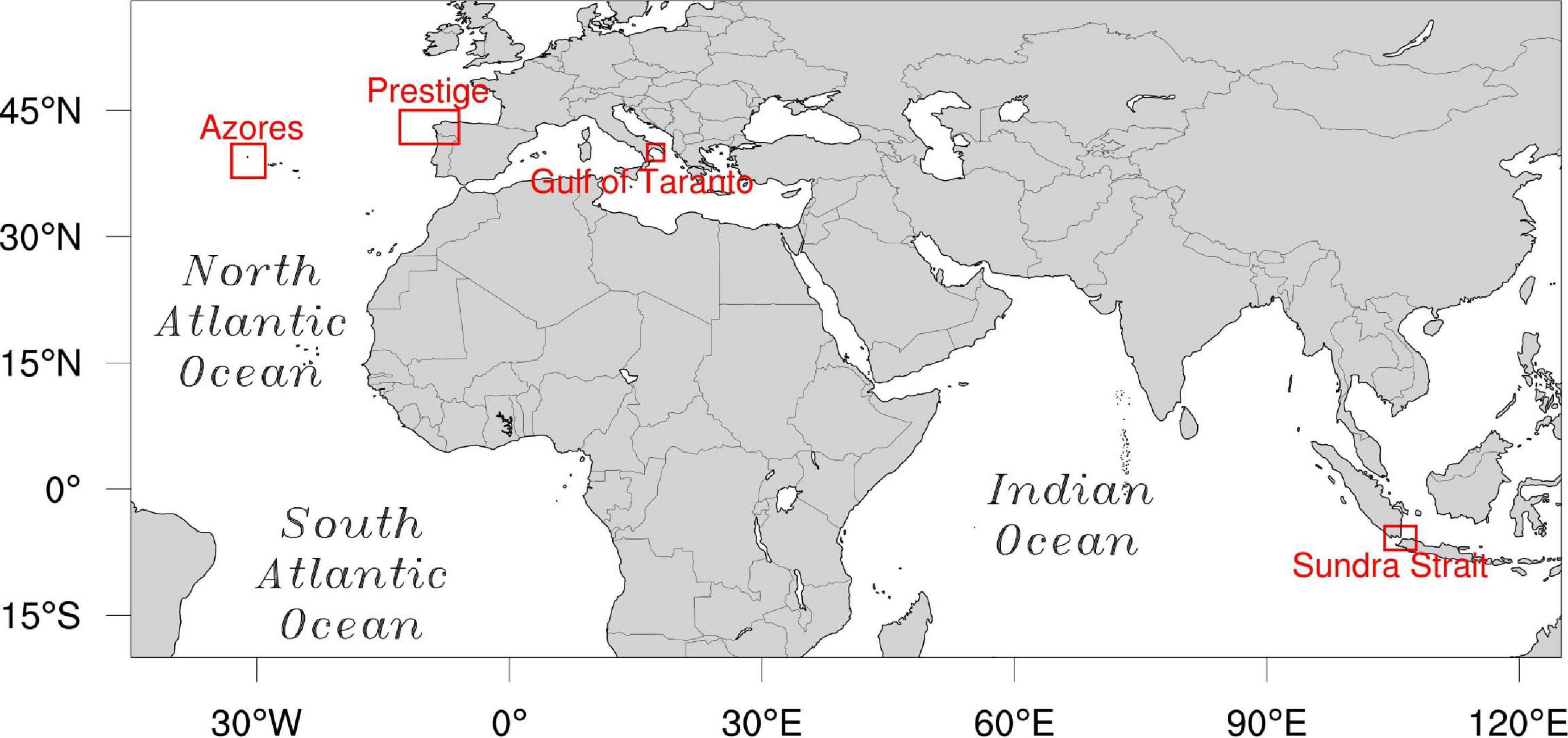
Figure 1. Areas of the four case-studies experiments. Red rectangles delineate the boundaries of the nested domains.
The SURF workflow connects numerical integration codes to several pre- and post-processing procedures, making each platform component easy to deploy in a limited region, which is part of the parent model domain in which SURF is nested. The initial nesting fields can be taken from operational analyses or reanalysis, forecast products, and hindcast products. These are available in the CMEMS catalog, but other data sources can also be used. Consequently, in nested models that are relocatable, the input parent data have to have a pre-defined standard format so that the initial and lateral boundary conditions can be automatically generated by the SURF platform modules, in particular the interpolation routines that consider the high-resolution coastline geometry.
Horizontal and vertical interpolation is a key feature of the nested model initialization procedure. SURF uses a method developed by De Dominicis et al. (2014), in which the coarser-resolution ocean fields are extrapolated using the sea-over-land (SOL) procedure. This routine uses a diffusive boundary layer approach that extrapolates the field values on the areas near the coastline where the parent model solutions are not defined. The SOL procedure iteratively computes the ocean quantities on the land grid-points, so that these quantities can be interpolated on the child grid. This also applies to atmospheric fields in order to avoid land contaminations near the land-sea boundaries. After SOL has been applied, a bilinear interpolation method is used for the structured grid, while the Cressman’s interpolation technique (Cressman, 1959) is used for the unstructured grid model component. A simple linear interpolation is used for vertical interpolation.
Structured and unstructured relocatable ocean model for forecasting can deal with several types of sources of ocean and atmospheric input data. In the current version the input atmospheric fields have to be defined on a regular (orthogonal) curvilinear spherical grid, while the input ocean fields can be defined on both a regular and non-regular (e.g., the global tripolar grid) curvilinear spherical grid and on an unstaggered and staggered Arakawa C grid.
The SURF platform contains all of the static auxiliary fields, such as the bathymetry and the tidal harmonic components, derived from the Oregon State University Tidal Prediction Software (OTPS, Egbert and Erofeeva, 2002) tidal model with a 1/30 horizontal resolution. Tidal components can be added both as the equilibrium tidal sea level and/or only at the lateral boundaries.
The model forecast fields of currents, temperature and sea level are post-processed and can then be interfaced with specific application models like Medslik-II oil spill transport and fate model (De Dominicis et al., 2013), a trajectory drift model (Jansen et al., 2016) and wave models, such as SWAN (Booij et al., 1999).
SURF-Structured Grid Component
The structured grid component of the SURF platform (SURF-S) is based on the finite differences hydrodynamic NEMO code v3.6 (Madec, 2016). This solves the three-dimensional (3D) primitive free-surface ocean equations under hydrostatic and Boussinesq approximations, along with turbulence closure schemes and a non-linear equation of state, which combines the two active tracers (temperature and salinity) with the fluid velocity. The 3D space domain is discretized by an Arakawa-C grid, in which the model state variables are horizontally and vertically staggered. In the vertical direction, a stretched z-coordinates transformation is used (z(k) = hsur-h0⋅k-h1log[cosh((k-hth)/hcr)]) which includes five free parameters hsur, h0, h1, hth, and hcr and defines a nearly uniform vertical location of levels at the ocean top and bottom with a smooth hyperbolic tangent transition in between (Madec, 2008). The bottom is approximated by partial cells (i.e., the bottom layer thickness varies as a function of position) to best fit the real bathymetry.
Here, we describe only the configuration parameters of NEMO that are automatically chosen for rapid nesting of SURF in CMEMS fields. However, an expert user can modify these specific choices, as NEMO allows for many other options (Madec, 2008). Density is computed according to Jackett and McDougall’s non-linear equation of state (Jackett and Mcdougall, 1995). A horizontal biharmonic operator is used for the parameterization of lateral subgrid-scale viscosity and diffusion for momentum and tracers. The horizontal eddy diffusivity and viscosity coefficients are parameterized as a function of the parent coarse resolution model. If a0 is the parent viscosity or diffusivity, the nested model equivalent coefficient is a = a0 (ΔxF/ΔxL)4, where ΔxF is the nested grid and ΔxL is the large-scale model grid spacing. The vertical eddy viscosity and diffusivity coefficients are computed following the Pacanowsky and Philander’s Richardson number-dependent scheme (Pacanowski and Philander, 1981). For cases in which unstable stratification is present, a higher value (10 m2/s) is automatically used for both the viscosity and diffusivity coefficients.
The Monotonic Upstream Scheme for Conservation Laws (MUSCL) is used for the tracer advection and the Energy and Enstrophy conservative (EEN) scheme for the momentum advection (Arakawa and Lamb, 1981; Barnier et al., 2006). No-slip conditions at closed lateral boundaries are applied and the bottom friction is parameterized by a quadratic law for the wall bottom stress. The surface heat and water fluxes are computed using specific bulk formulas, as described by Pettenuzzo et al. (2010). The momentum flux is written as a true stress and it uses the Hellermann and Rosenstein (1983) drag coefficient formulation.
For the lateral open boundary conditions, specific formulations are used, depending on the model variables. For barotropic velocities, the Flather scheme (Oddo and Pinardi, 2008) is used, while for baroclinic velocities, active tracers, and sea surface height, the flow relaxation scheme is used Engerdahl (1995). Tidal barotropic forcing (ssh and velocity) can also be add to the barotropic velocity at the open boundaries. To preserve the total transport after horizontal and vertical interpolation, an integral constraint method is applied (Pinardi et al., 2003).
SURF-Unstructured Grid Component
The unstructured grid component of the SURF platform (SURF-U) is based on the finite element hydrodynamic SHYFEM code (Umgiesser et al., 2004). This is a 3-D finite element hydrodynamic model that solves the primitive equations under hydrostatic and Boussinesq approximations. The unstructured grid is an Arakawa B with triangular meshes, which provides an accurate description of irregular coastal boundaries. The scalars are computed at grid nodes, whereas velocity vectors are calculated at each element center. A layer discretization is applied in the vertical and the temperature, salinity, currents and pressure variables are computed at the center of each layer, whereas stress terms and vertical velocities are solved at the layer interfaces. The choice of layer thicknesses in each configuration is as homogeneous as possible, to increase the accuracy of the second order centered vertical finite difference scheme.
A specific characteristic of unstructured meshes is their ability to represent several scales seamlessly, reaching higher resolution where necessary. The horizontal mesh is created by using advanced and customized meshing tools, allowing higher grid resolution approaching the coastal waters. The tools are based on GMSH2 and BLENDER3 software, which are embedded into the SURF platform.
The model uses a semi-implicit algorithm for integration over time, which has the advantage of being unconditionally stable for gravity waves, bottom friction, and Coriolis terms, and allows transport variables to be solved explicitly. The Coriolis term and pressure gradient in the momentum equation, and the divergence terms in the continuity equation, are treated semi-implicitly. Bottom friction and vertical eddy viscosity are treated fully implicitly for stability reasons, while the remaining terms (advective and horizontal diffusion terms in the momentum equation) are treated explicitly. These choices enable the rapid implementation of the model, but an expert user can change them to others if necessary.
The air-sea heat and water fluxes are parameterized by the bulk formulas described by Pettenuzzo et al. (2010), while the surface stress is computed with the wind drag coefficient according to Hellermann and Rosenstein (1983). Horizontal eddy viscosity is computed by the Smagorinsky (1963) formulation. For the computation of the vertical viscosities and diffusivities, a k–e turbulence scheme is used, adapted from the General Ocean Turbulence Model (GOTM) described by Burchard and Petersen (1999). For the lateral open boundary conditions, the sea level is set at open boundaries nodes with a Dirichlet condition, while the total velocities are relaxed to the inner buffer zone of the computational grid. A Dirichlet boundary condition is set for the active tracers if the flow enters the domain, while a zero-gradient condition, based on the weighted average of closest internal values, is imposed in case of outflow. Further information on numerical features could be found in Federico et al. (2017).
Other Relocatable Ocean Modeling Platforms
After the pioneering work of the Harvard Ocean Prediction System (HOPS, Robinson, 1999), several other platforms were developed for the rapid deployment of high-resolution models. The last application of HOPS is reported in De Dominicis et al. (2014), after which the model was dismissed and an upgraded version of it is now available as MSEAS (Haley and Lermusiaux, 2010). The model is baroclinic, containing accurate and new numerical schemes with respect to HOPS. It has been validated in several areas of the world’s ocean (Lermusiaux et al., 2011, 2017). A key difference is that SURF offers both structured and unstructured grid models.
The United States Naval Research Laboratory’s RELOcatable ocean nowcast/forecast system (RELO) system includes both structured and unstructured grid models: RELO-NCOM based on the Navy Coastal Ocean Model (NCOM; Martin, 2000) and RELO-ADCIRC based on the three-dimensional, finite-element ocean model (ADCIRC, Luettich and Westerink, 2004). It provides for relocatable ocean forecasting and data assimilation, which is used for operational forecast support for antisubmarine warfare, intelligence, surveillance, and reconnaissance, Navy special operations and other applications have been tested both in open ocean and in complex coastal regions. RELO is not open source and it is not made available as an overall platform.
A revised version of HOPS that considers ROMS (Shchepetkin and McWilliams, 2003, 2005) and a correction scheme for temperature and salinity data was published by Onken (2017). It uses a curvilinear orthogonal grid, which is not suitable for coastal region geometries, and it does not allow rapid nesting in a large scale baroclinic model.
The OPENCoastS platform (Oliveira et al., 2020) is barotropic and thus it can only be used for coastal forecasting. The output consists only of sea level and barotropic currents, consequently no steric effects or river plumes can be considered. The platform is based on an unstructured-grid model (Zhang et al., 2016).
Being a relocatable platform SURF has two major advantages over the products outlined above: (i) a robust grid interpolation scheme and lateral boundary constraints (Pinardi et al., 2003); (ii) a direct interface to the CMEMS service products (no need of any reformatting for the ocean fields) that are open and free every day, in every part of the ocean. This makes SURF one of the most complete open-source and freely available relocatable platforms, offering several grid and numerical scheme solutions, nested in an operational global model with high accessibility and trusted repositories.
Case Study 1: Drifter Trajectories in the Taranto Seas
The Taranto Seas are a set of interlinked embayments, the larger of which covering a 7.5 km-wide elliptical embayment with dominant estuarine dynamics (De Pascalis et al., 2015), The larger embayment, called simply the Taranto Sea, is linked to the Taranto Gulf open sea and is an area of relatively intense tidal currents. Complex dynamics characterize the offshore areas of the Taranto Gulf, with basin-wide gyre reversals (Federico et al., 2020) that drive opposite current directions in the near-shore. Thus, a high resolution is required for the Taranto Sea while simultaneously keeping the connection with the open sea area currents. This is a typical downscaling problem and is particularly suitable for an unstructured grid model. The unstructured-grid component of the modeling platform SURF-U was implemented in the Gulf of Taranto (Figure 2, left panel) with higher resolution elements for the Taranto Seas (Figure 2, right panel). The downscaled currents interface with a Lagrangian drift modeling system (Jansen et al., 2016), designed for search-and-rescue support. The model results are compared with CTD, ADCP, tide-gauge data and drifter trajectories, collected in October 2014 during the Marine Rapid Environmental Assessment (MREA14) oceanographic survey (Pinardi et al., 2016).
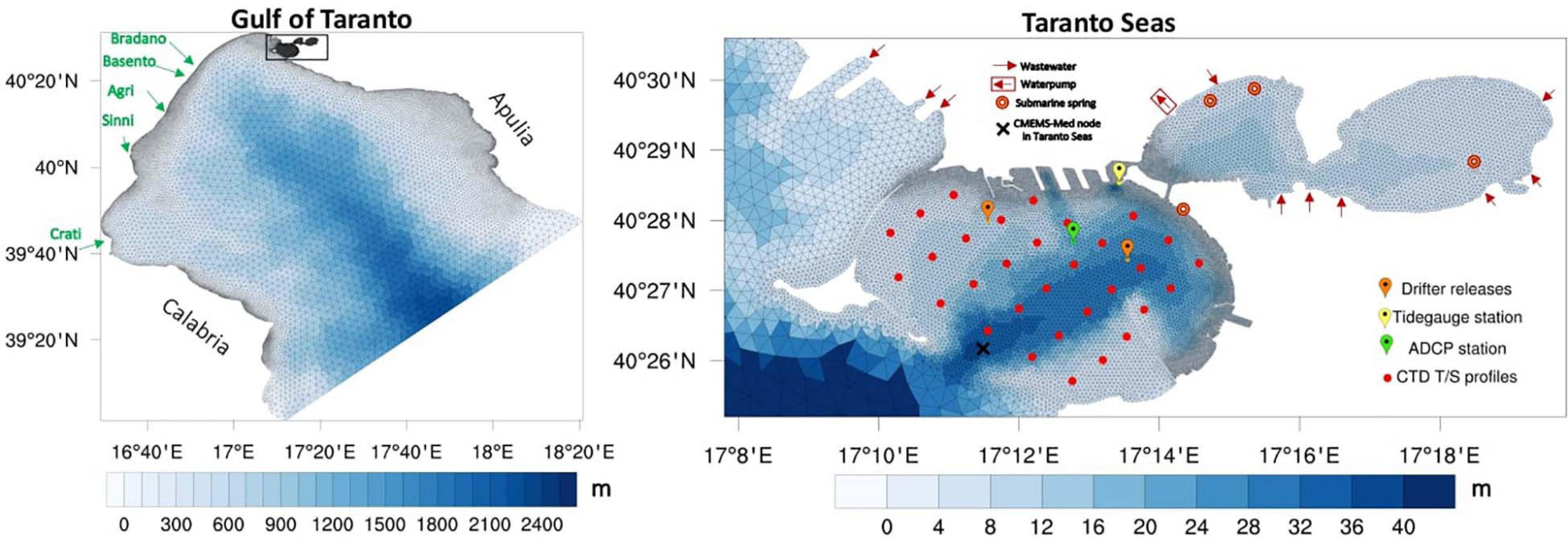
Figure 2. Case study 1: SURF-U horizontal grid with bathymetry overlapped for (left panel) the whole domain (Gulf of Taranto) and for (right panel) Taranto Sea. Red, green, yellow, and orange dots denote the locations of the CTD, ADCP, tide-gauge data and drifter releases, respectively.
Model Set-up
The horizontal resolution of the SURF-U unstructured grid ranges from 3 km in open seas to 100 m in the coastal waters and down to 20 m in the Taranto Sea. The bathymetry was derived from the EMODNET4 product at 1/8 × 1/8 arc-minutes (about 230 × 230 meters) resolution for open seas and coastal waters. This bathymetry was integrated with higher-resolution bathymetry (resolutions of an order of 1 m) for the coastal areas of Taranto, provided by the Italian Navy Hydrographic Institute. In the vertical, the layer thicknesses are 2 m from the sea surface down to 90 m and then progressively (stepwise) increase toward the bottom with a maximum layer thickness of 200 m starting from 1000 m of depth. The initial (temperature and salinity fields) and lateral boundary conditions (temperature, salinity, total velocity, and non-tidal sea surface height) are obtained from the Mediterranean component of CMEMS (MEDSEA_ANALYSIS_FORECAST_PHY_006_013, Clementi et al., 2019) providing analyses and 10 days forecasts. The tidal elevation is added to the non-tidal CMEMS sea surface height at each boundary node of the domain. Eight of the most significant constituents are considered: M2, S2, N2, K2, K1, O1, P1, and Q1. The surface forcing is derived from European Centre for Medium-Range Weather Forecasts (ECMWF) analysis products with 1/8-degree horizontal resolution and 6-h frequency. The set-up is completed by adding the rivers, wastewater, and spring source inputs. The monthly mean discharges (from Verri et al., 2018) of the five main rivers (Bradano, Basento, Agri, Sinni and Crati, as reported on the left panel of Figure 2) are imposed on the western coastline. Due to the lack of available observations, river inflow salinity is set to a constant value of 0.1 PSU. Wastewater, water pump outflow, and submarine springs in the Taranto Seas are applied as discharge, salinity, and temperature fields following De Pascalis et al. (2015). Appendix Table A2 summarizes the values for the model input parameters selected for this experiment.
The currents of SURF-U in the Taranto Sea are provided to the Lagrangian drifting objects model of Jansen et al. (2016). This is a 2D and 3D particle transport model, which integrates the particle advection equation using a 4th order Runge-Kutta method. For this case study, the Lagrangian model is configured to model surface drift using the uppermost model layer currents.
Results
A 10-day simulation (27 September – 07 October 2014) was conducted using the SURF-U model described above for the Taranto Sea. The first 3 days of simulation are considered as the spin-up time necessary for the downscaled model to produce dynamically adjusted fields after initialization from the CMEMS model variables. Figure 3 shows the model comparison between SURF-U and CMEMS and the temperature CTD data collected during the MREA14 survey. The spatial distribution of the CTD profiles (red circles on the right panel of Figure 2) is very dense (spacing between the stations is less than 1 km), due to the need to sample the coastal and local scale features. The 31 CTD temperature casts have been averaged to produce a representative profile of the Taranto Sea, as reported in the left panel of Figure 3, together with the modeled profiles. SURF-U is close to the observed temperature profile, showing a significant improvement in terms of the coarse resolution CMEMS analyses, as represented by a single grid point located near the entrance of the Taranto Sea (see the black cross in the right panel of Figure 2). The improvement is evident in the BIAS profile (Figure 3, center panel), which is 0.13 C for SURF-U and is 0.3 C for CMEMS. For the RMSE profile (Figure 3, right panel) values of 0.15 C and 0.32 C are obtained for SURF-U and CMEMS, respectively.
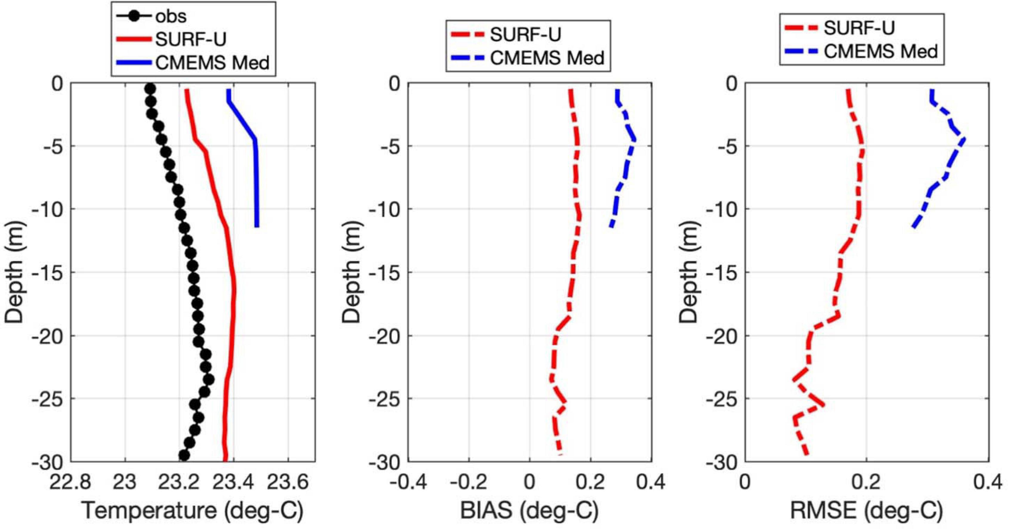
Figure 3. Comparisons between modeled (SURF-U and CMEMS Med) and observed CTD temperature profiles (left panel), with BIAS (middle panel) and RMSE (right panel). The observed temperature (black dotted line) is an average profile over the 31 CTD stations collected during the MREA14 survey in the Taranto Sea.
Structured and unstructured relocatable ocean model for forecasting-U performs better than CMEMS for several reasons: (i) the finer horizontal and vertical resolution, (i) the higher-resolution of coastlines and bathymetry, (iii) numerical settings specific to the coastal zones (e.g., turbulence closure models), (iv) realistic input of freshwaters discharging into the Taranto Sea system. However, there are still missing processes in the SURF-U forecast such as the coupling between currents and Stokes drift and the use of high-frequency atmospheric forcing.
The model is compared to a tide gauge station and ADCP currents in Figure 2 (right panel). The top panel of Figure 4 shows a remarkable similarity between the SURF-U fields and the observations, demonstrating that SURF-U is capable of propagating the tidal sea level from the lateral open boundary condition to inshore (the sea level RMSE of SURF-U calculated over the whole time series is 0.15 cm).
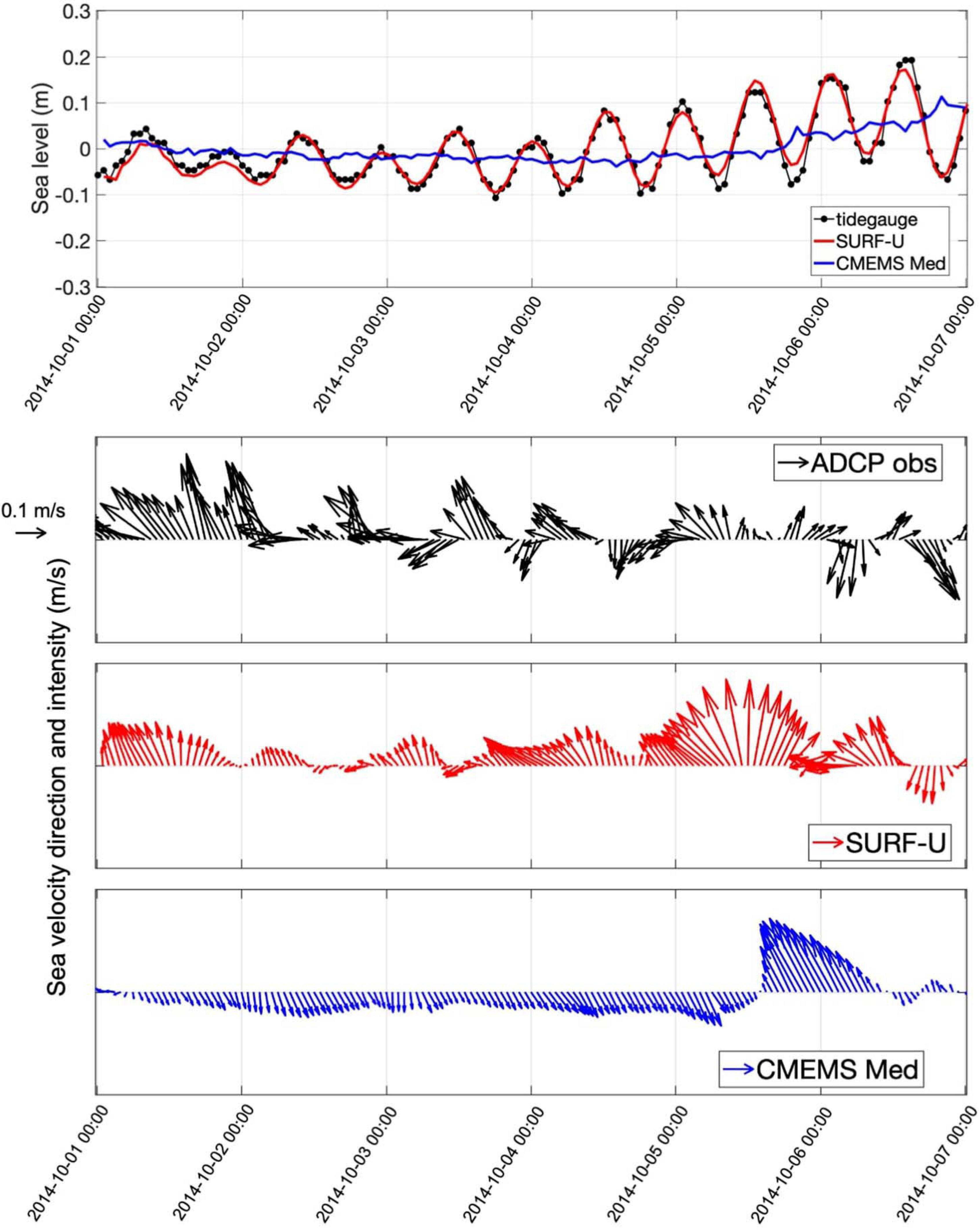
Figure 4. A comparison between modeled (SURF-U and CMEMS MED) and measured sea levels from tide-gauge (top panel). Time series of sea velocity direction and intensity, as measured by ADCP (black rows) and modeled by SURF-U (red rows) and by CMEMS Med (blue rows) (bottom panel) are given. The locations of the tide-gauge and ADCP stations are reported in Figure 2 right panel.
Figure 5 shows the mean trajectories of two groups of drifters released in the positions indicated in the right panel of Figure 2, for the first 12 h after their release (5 October 2014). The observed trajectory is shown in black and is compared to those simulated by the Lagrangian model using the SURF-U and CMEMS model data. The CMEMS data are derived from the single grid point outside the Taranto Sea (black cross on the right panel of Figure 2), chosen ad hoc for the simulation. For the eastern group of drifters, the SURF-U trajectory shows a significant improvement, while for the western group the SURF-U and CMEMS drifts are equivalent. This could be due to limitations in our modeling hypothesis, such as the low spatial/temporal variability of wind forcing and the neglected effects of Stokes drift. However, the inherent limited predictability of objects floating at sea can only be ameliorated by ensemble methods (Vieira et al., 2020).
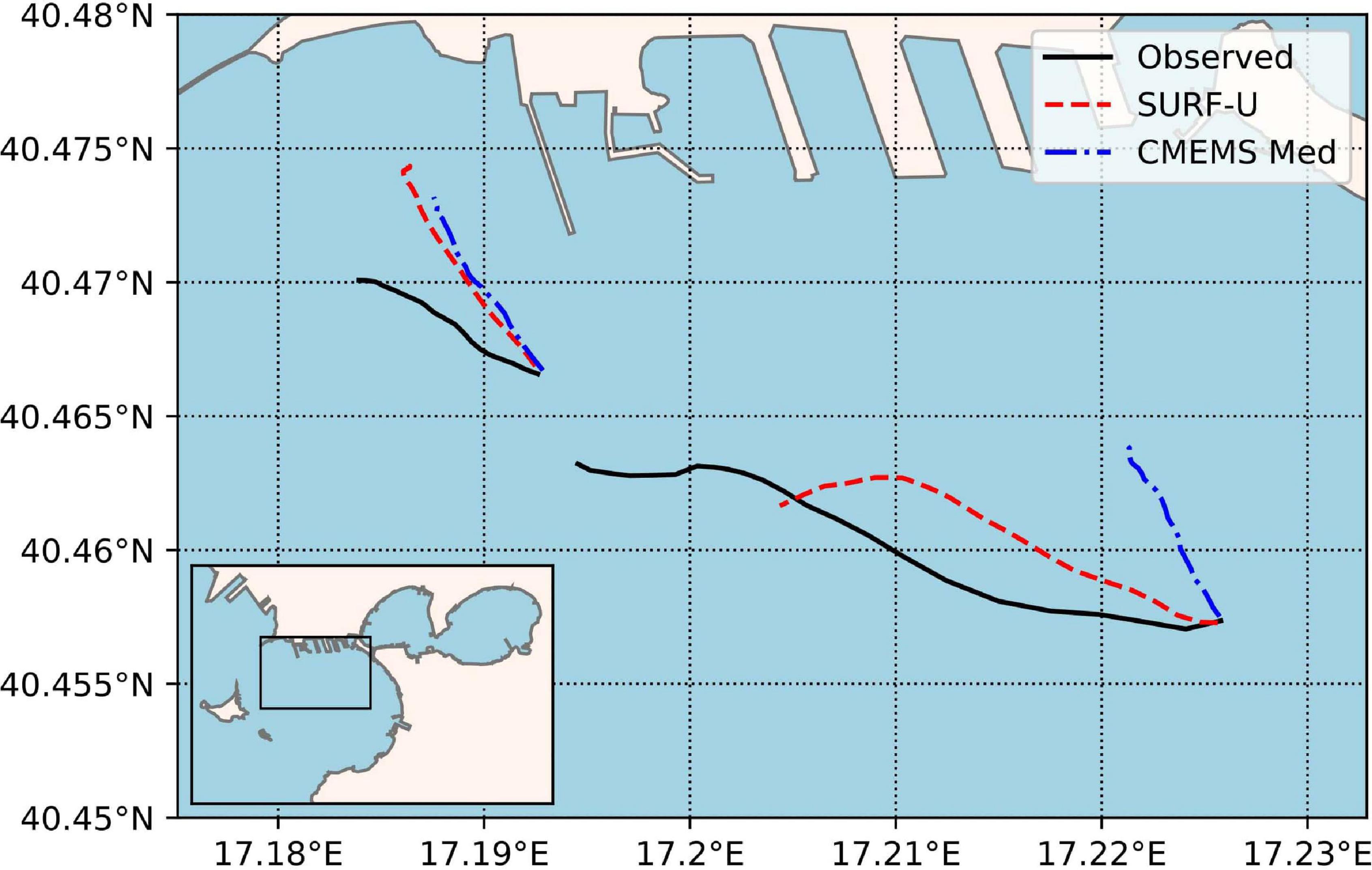
Figure 5. Mean drifter trajectories of the two drifter groups released in the Taranto Sea (black), and simulated drifter trajectories using the SURF-U (red) and CMEMS Med (blue).
Case Study 2: Storm Surges in the Azores Archipelago
The Corvo and Flores islands experienced the impact of Hurricane Lorenzo. This broke records when it briefly powered up to a Category 5 on the Saffir-Simpson scale on 28 September 2019, when it was 2.270 km southwest of the Azores Islands, with winds peaking at 260 km/h. No other tropical cyclone formed in the Atlantic Ocean has reached such high intensity so far north since records began in 1851. Lorenzo then weakened to a Category 2 with winds of 165 km/h and hurtled toward the Azores on 2 October in the early morning. The unstructured-grid component of the modeling platform SURF-U was implemented in a subregion of the mid-Atlantic Ocean with specific higher resolution around Corvo and Flores islands, within the Azores archipelago. The aim was to assess the capability of the model in simulating extreme events, such as storm surges due to the passage of hurricanes.
Model Set-up
The SURF-U unstructured grid covers the mid-Atlantic region approximately delimited by the geographical coordinates [−33W, −29W] [37W, 41N] and including the Corvo and Flores islands of the Azores archipelago. The horizontal resolution ranges from 3 km in the open sea to 500 m in the coastal waters of each island. The bathymetry was derived from the GEBCO5 product at a resolution of 30 arc-seconds (about 830 × 830 meters). The vertical z-layers are selected to be 2 m from the surface up to a maximum of 200 m from 1000 m from the bottom. The initial and lateral boundary conditions are obtained from the Global component of the CMEMS analysis products (GLOBAL_ANALYSIS_FORECAST_PHY_001_024). To assess the sensitivity of the storm surge to atmospheric forcing, two experiments were performed using the NOAA-NCEP (with a 1/4-degree horizontal resolution and 6 h of frequency) and ECMWF (with a 1/10-degree horizontal resolution and 3 h of frequency) analysis products. The simulation with ECMWF is referred to as SURF-U-E while that with NCEP is SURF-U-N. Appendix Table A3 summarizes the values for the model input parameters chosen for this experiment.
Results
A simulation over 10 days (27 September – 07 October 2019) was conducted using the SURF-U platform. Like in the previous test case, the first 3 days of simulation were considered the spin-up time necessary for the downscaled model to produce dynamically adjusted fields after initialization from the CMEMS ocean model variables.
According to a National Hurricane Center (NOAA-NHC) report (Zelinsky, 2019), hurricane Lorenzo had a rapid passage in the north-western part of the downscaled model domain, which is evident in the track (Figure 6, top-right panel) indicating the locations of hurricane pressure minima every 6 h. On 2 October at 06:00 am, the hurricane eye was 40 km from the Azores’ westernmost islands. The highest wind speeds recorded by the meteorological stations in Flores and Corvo (Zelinsky, 2019) were 97 km/h (at 04:30 am) and 119 km/h (at 06:00 am), respectively.
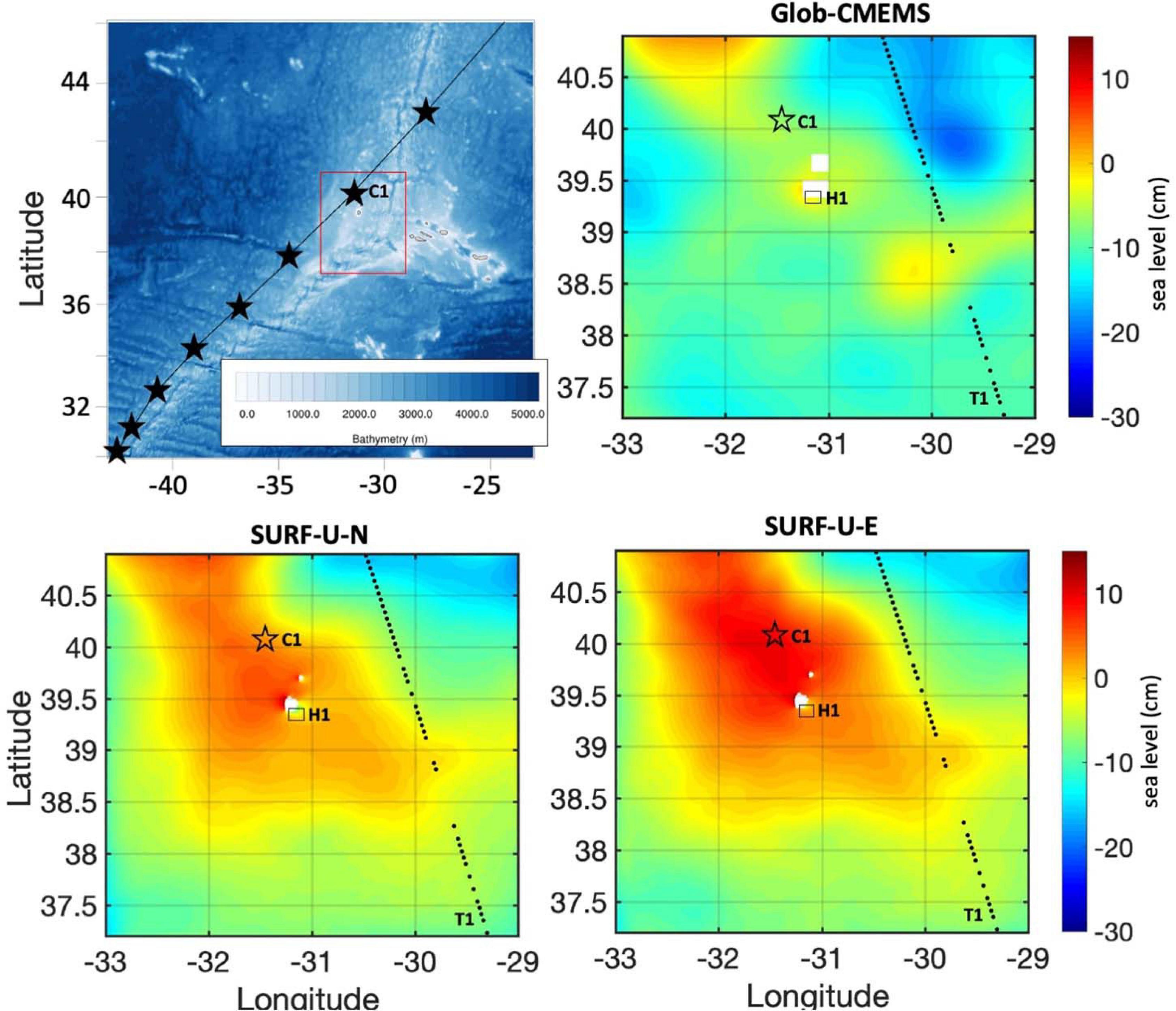
Figure 6. (Top-left panel) Track of hurricane Lorenzo (line with stars) in the area of the Azores archipelago (red box indicates the SURF-U model); the locations of hurricane pressure minima are indicated every 6 h. Star labeled C1 is the hurricane eye on 2 October at 0600am. (Top-right panel) Map of sea surface height on 2 October at 0600am (C1 hurricane time) for Glob-CMEMS. Sea level for SURF-U-N (bottom-left panel) and SURF-U-E (Bottom-right panel). Altika satellite track (from SEALEVEL_GLO_PHY_L3_REP_OBSERVATIONS_008_062 CMEMS dataset) is indicated by T1. The H1 box identifies the commercial port of Lajes in Flores.
The bottom- and top-right panels of Figure 6 show the sea surface height on 2 October at 06:00 am for CMEMS, SURF-U-N and SURF-U-E. Both SURF-U configurations show an increase in sea level with respect to CMEMS in the area surrounding the two islands, in the open ocean and the coastal areas. Outside of the hurricane impact area, similar features between the parent and downscaled models are noticeable, except for the cyclonic core at [−29.8W, 39.8N], which is not present in SURF-U. The comparison between the two SURF-U experiments shows that SURF-U-E produces a higher sea level, because the wind intensity is greater in the ECMWF data, with a maximum wind speed at 06:00 am of 143 km/h compared to 101 km/h in the NCEP data.
As no in situ oceanographic data were available for the area and period of interest, satellite altimetry products (SEALEVEL_GLO_PHY_L3_REP_OBSERVATIONS_008_062) were used to validate the results in the open ocean. The Altika satellite track (T1 in Figure 6, bottom and top-right panels) crossed the area on 2 October at 07:28 am. Figure 7 shows a comparison between the satellite absolute dynamic topography and the sea surface height from the two SURF-U implementations. The satellite sea level view shows a high level of variability along the track, which is not well reproduced by the models. The correlation between sea levels in the models and the satellite is relatively low, with values of 0.45, 0.35, and 0.28 for SURF-U-E, SURF-U-N, and CMEMS, respectively, but remain higher in the SURF-U simulations.
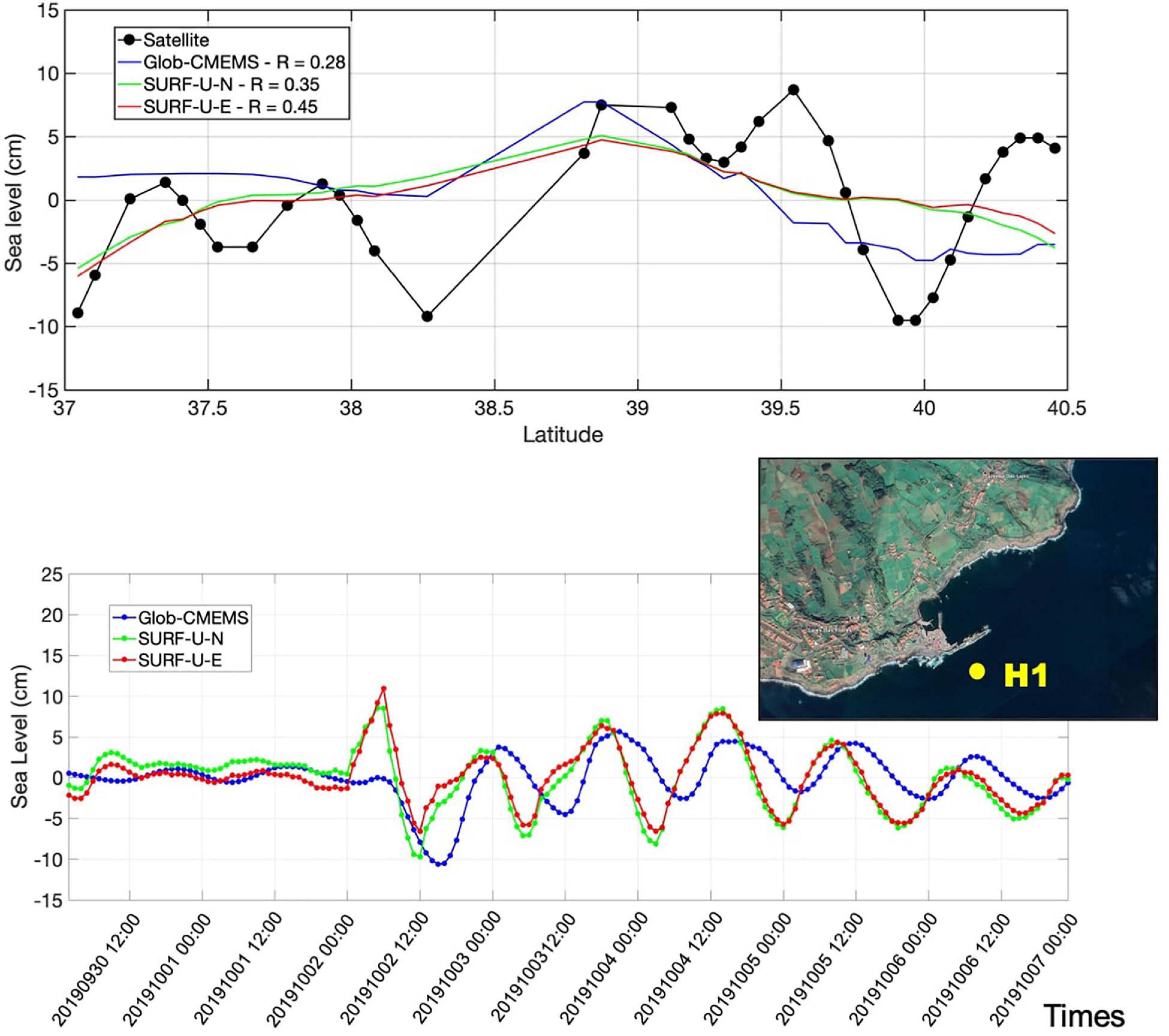
Figure 7. Comparison between the satellite absolute dynamic topography and the sea surface height from the CMEMS and the two SURF-U models (top panel). The time series of the sea level for Glob-CMEMS, SURF-U-N, and SURF-U-E close to the commercial port of Lajes in Flores (bottom panel) are shown.
Figure 7 shows the storm surge at the coastal scale near the commercial port of Lajes in Flores (H1 box in Figure 7), where extensive damage and the total destruction of the port were reported by Zelinsky (2019) in this period. The time series of SURF-U show a local increase of sea level from 01:00 am on 2 October, with a maximum peak at 06:00 am. This feature is not present in CMEMS sea level. Since CMEMS and SURF-U were forced by the same atmospheric field (ECMWF), we argue that this difference is due to the higher resolution of the coastal model and to the different wind stress parametrizations in the two models. SURF-U-E indicates a higher surge (12 cm) than SURF-U-N (8 cm) at the peak event. The patterns of the three models after the hurricane impact are similar, with a large decrease immediately after the passage, then sea level oscillation and adjustment, until reaching normal conditions. This feature has previously been reported by several authors (Ezer, 2019).
Case Study 3: The Prestige Oil Spill Accident in the Galicia Coast
On 13 November 2002 at 15:00, the tanker Prestige, carrying a total of 77,000 tonnes of heavy fuel oil on board, began to spill oil 55 km away from the north coast of Galicia (northwest Spain) (Figure 8). In anticipation of the arrival of oil in the coastal zone, the authorities decided to take the ship far from the Spanish coast. On 19 November 2002 at 8:00, after several days of sailing adrift (red line on Figure 8), the vessel collapsed about 250 km west of the Spanish coast, breaking in two pieces and sinking. Although the total amount of oil released into the environment is unknown, it is believed to be more than 60,000 tonnes of heavy fuel, polluting thousands of kilometers of coastline in Spain, France, and Portugal (Balseiro et al., 2003).
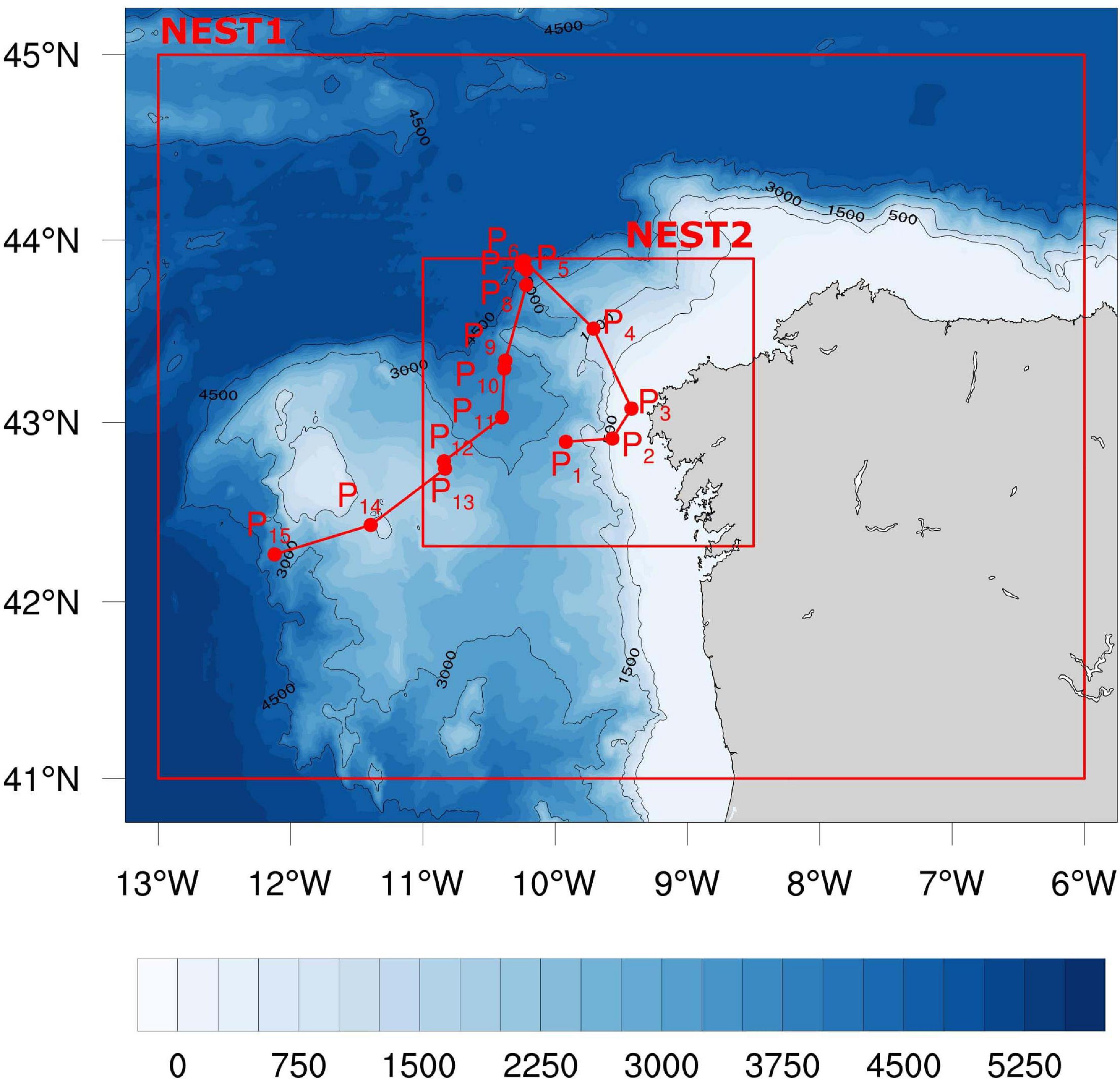
Figure 8. Bathymetry contour map of the Prestige experiment area. Red rectangles delineate the boundaries of the two consecutive nested domains with increasing grid resolutions of 2000 and 500 m (from the outer to the inner domains). Red dots denote the Prestige Ship’s positions from the initial spill (P1) on 13-11-2002 15:10 to the final breaking up (P15) on 19-11-2002 08:00. The list of the Prestige’s positions are reported in Table 1.
The structured-grid component of the SURF platform (SURF-S) was implemented for the offshore waters of the Spanish northwest coast (Figure 8) to show the importance of downscaling in the simulation of the oil drift. The SURF-S currents were combined with the Medslik-II oil spill model (De Dominicis et al., 2013) to simulate the Prestige oil spill evolution from the initial spill on 13 November 2002 at 15:00 UTC to 19 November 2002 at 8:00 UTC. The oil spill model results were compared with the Envisat satellite SAR image available for 17 November 2002 at 10:45 UTC (Figure 9, top-left panel) when the spill had already reached the Spanish coast.
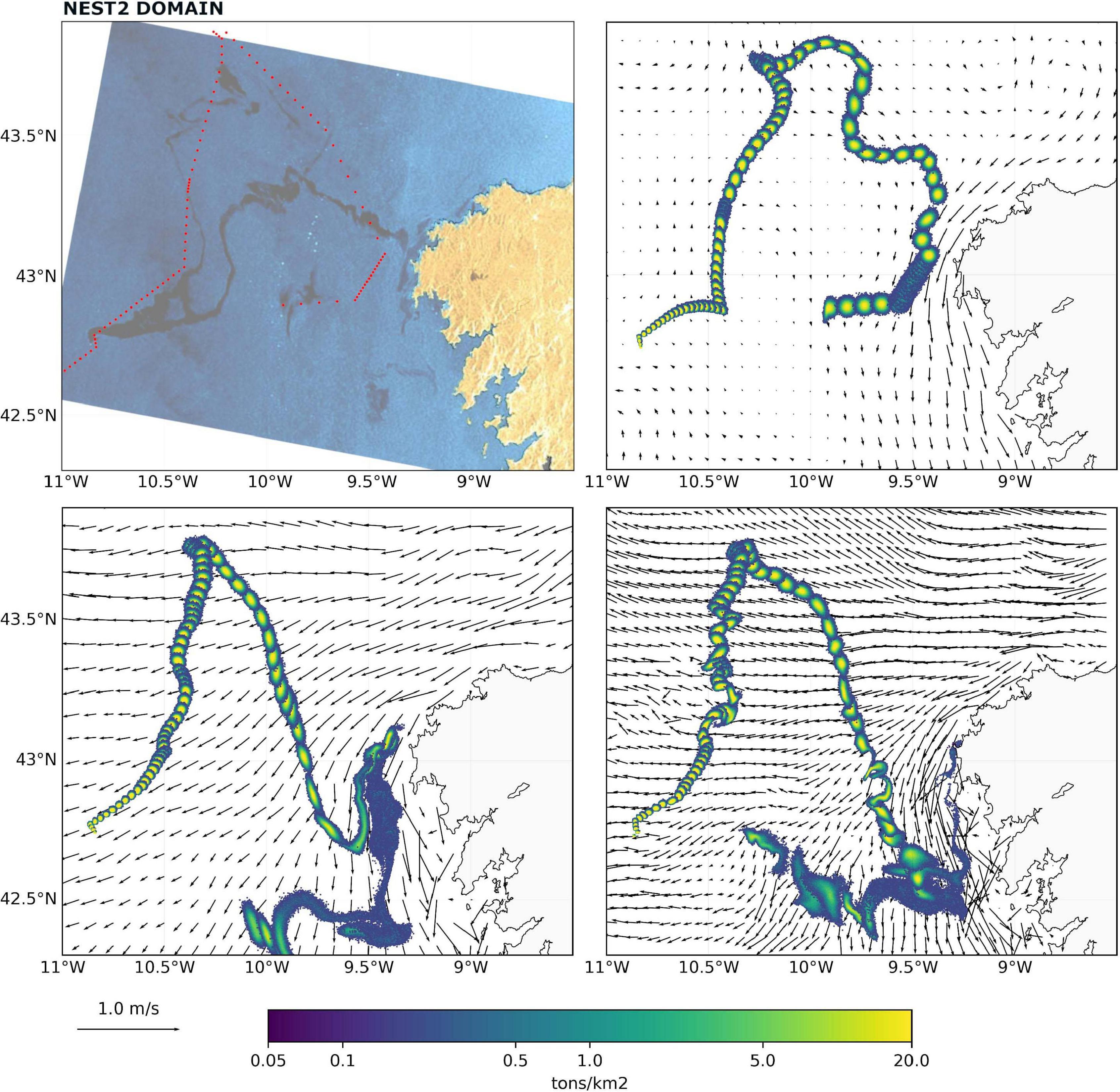
Figure 9. ESA Satellite image of 17 November at 10:45 (top-left panel) showing the wake of fuel oil in black. Red dots indicate the location of the release points assumed. Simulated drift of a continuous leak of fuel oil along the trajectory taken by the Prestige from 13 November at 15:00 to 17 November at 11:00 forced by 3 different model CMEMS (top-right panel), NEST1 (bottom-left panel), and NEST2 (bottom-right panel) with increasing grid resolutions of 8000, 2000, and 500 m. Black arrows, whose length is proportional to velocity, denote the direction and strength of the ocean currents. Arrows are subsampling every 1 (CMEMS), 4 (NEST1), and 10 (NEST2) grid points.
Model Set-up
A double nested model experiment was conducted (NEST1 and NEST2). Appendix Table A4 summarizes the values for the model input parameters chosen for this experiment. For each nesting, the grid spacing was decreased by a factor of 4. In this case we used CMEMS reanalysis fields (IBI_REANALYSIS_PHYS_005_002 products) because no analyses were available for such period. The starting CMEMS fields are at 1/12° horizontal resolution. The NEST1 model domain covered an area of approximately 552 km in longitude by 447 km in latitude, extending from 13.0° W to 6.0° W and from 41.0° N to 45.0° N, with a resolution of 1/48° (∼1638 × 2316 m). The NEST2 domain extended approximately 200 × 177 km from 11.0° W to 8.5° W and from 42.312° N to 43.9° N, with a resolution of 1/192° (∼417 m × 579 m).
This case study investigated the effect of increasing horizontal resolution while maintaining the same vertical resolution in both nested models. Each nested domain consists of 120 z-levels with a stretching factor of hcr = 30 and a model level with maximum stretching of hth = 60. The locations of the vertical levels, defined from a reference coordinate transformation (see Section “SURF-Structured grid component”), were smoothly distributed from 0.5 m to a maximum depth of 2426.8 m and had level thicknesses that increased with depth from 1 to 89 m. Bathymetry was obtained from the General Bathymetric Chart of the Oceans (GEBCO) datasets by linear interpolation of depth data into the SURF model grid. This dataset contains the bathymetry at a 30 arc-seconds resolution defined on a regular horizontal grid and covering the globe.
The initial and lateral boundary conditions for NEST1 were extracted from the reanalysis daily mean dataset of the Iberian-Bay of Biscay-Ireland component of CMEMS (IBI_REANALYSIS_PHYS_005_002 products), while for NEST2 they were obtained from the NEST1 downscaled fields. A spin-up of 3 days for the two consecutive nested models was considered. The NEST1 simulation started on 7 November 2002 at 00:00 and ran until 17 November 2002 at 24:00. The NEST2 simulations started at 00:00 UTC on 10 November 2002 and ran until 17 November 2002 at 24:00 UTC. The atmospheric fields used to force the two nested models were from ECMWF operational analyses, with a spatial resolution of 0.25° and 1-h temporal resolution. The list of the model input parameters together with the reference model values are given in Appendix Table A5.
The NEST1 and NEST2 model outputs are then provided to the oil spill model Medslik-II (De Dominicis et al., 2013), which can then be used to simulate the transport and weathering of the Prestige oil spill disaster. Medslik-II is an oil spill model that solves an advection-diffusion equation for the oil concentration and its transformation processes. Medslik-II requires the wind velocity, sea surface temperature, and sea currents as inputs, to compute the transport and transformation processes. Wind velocity components are provided by the ECMWF fields, as used in the hydrodynamic model. When modeling the Prestige oil spill, the release points was set based upon ship’s positions reported by the Bahamas Maritime Authority (Table 1). It is assumed that oil was spilled uniformly along the ship’s path with hourly release points (red dots in Figure 9) from the initial spill on 13 November at 15:00 UTC to the sinking point on 19 November, 8:00 UTC. Assuming that 60.000 tonnes of heavy/residual fuel oil were spilled, an oil spill rate value of 438 tonnes/hours for each release point was assumed. The heavy fuel-oil (M-100 type) was assumed to have a viscosity of 100.000 cSt at 15°C, and a measured density of 0.992 kg/L at 15°C (API gravity of 11.04) (Albaigés et al., 2006). The list of all Medslik-II input parameters is reported in Appendix Table A5 where the default values (De Dominicis et al., 2013) have been assumed for most of the parameters.
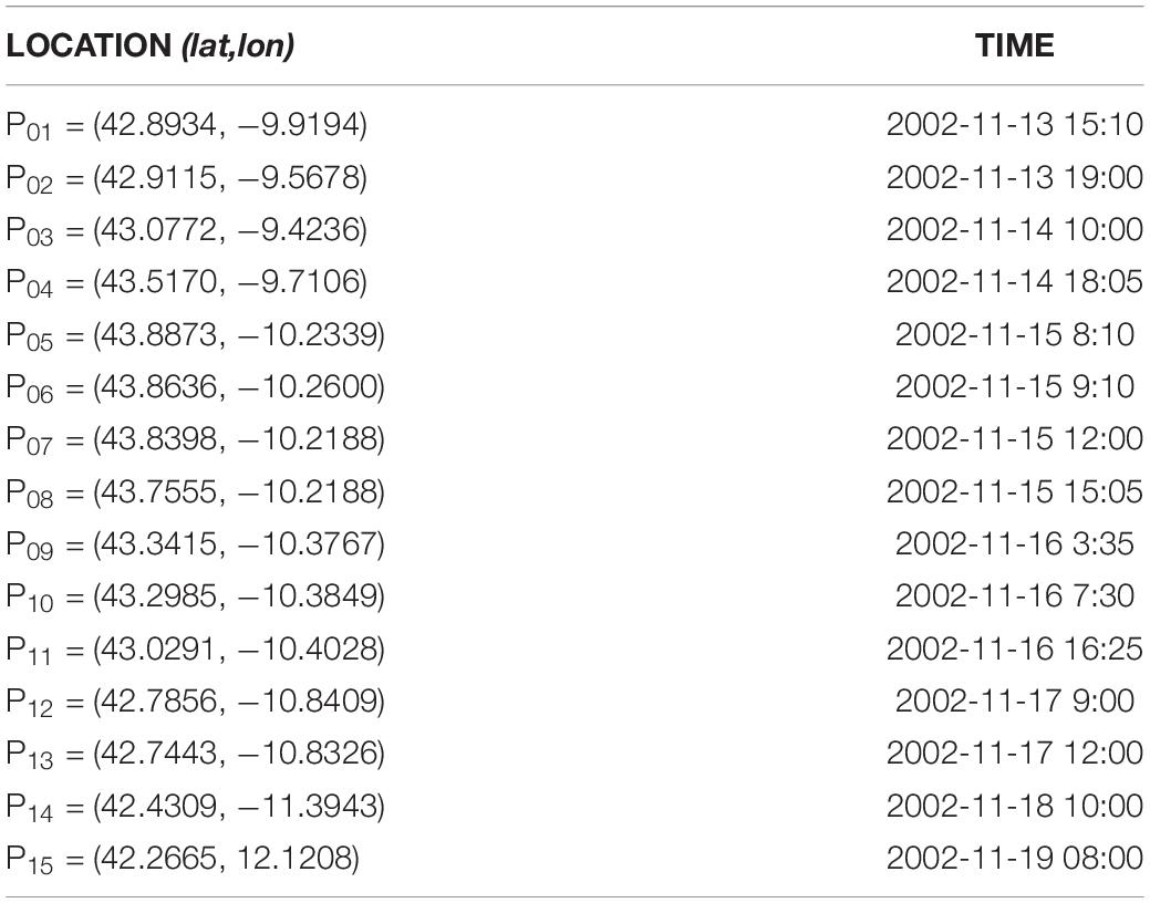
Table 1. The list of the Prestige’s positions reported by the Bahamas Maritime Authority Report from the initial spill to its final breaking up.
Results
The oil concentration simulated with the currents from CMEMS, NEST1, and NEST2 on 17 November 2002 at 11:00 UTC is shown in Figure 9, together with the ESA’s Envisat satellite image on the same date at 10:45 UTC.
The observed image and the simulation results have similarities in terms of the general oil slick shape. The oil spill simulation results show that the flow field generated by NEST1 and NEST2 is more intense than the parent CMEMS flow. This increase in surface current speed and the presence of finer-scale motion are responsible for the different oil spill surface concentrations obtained. The simulation with CMEMS shows that the oil remains close to the ship track release points at all given times, while in NEST1 and NEST2 the oil diffuses more realistically around the ship track release points. In addition, the NEST2 simulation shows that oil arrives at the coast, as confirmed by the satellite imagery.
However, the comparison between the model and satellite image indicates that all the simulations fail to predict that the oil slick split into two branches around 10.5W and 43.75N. Carracedo et al. (2006) suggested that the two branches could be formed due to the presence of two different types of oil with different densities that drifted at different depths. In our modeling exercise, we did not consider these different oil densities, and therefore this could be an explanation for the missing oil slick trajectory.
Case Study 4: The Sunda Strait
The Sunda Strait lies between the Indonesian islands of Java (to the south-east) and Sumatra (to the north-west) and connects the Java Sea (Pacific Ocean) to the Indian Ocean (south) (Figure 10, left panel). The Strait has a width of 24 km and the depth ranges from 20 m to 90 m, with the shallow part near the small Sangiang Island located in the middle part of the strait, as shown in the left panel of Figure 10. The Sunda Strait is considered to be a water area with one of the highest ship traffic densities in the world, serving both national and international shipping. Knowledge of the characteristics of the ocean currents in this Strait is essential for the safe navigation, planning, and development of the nearby coastal areas.
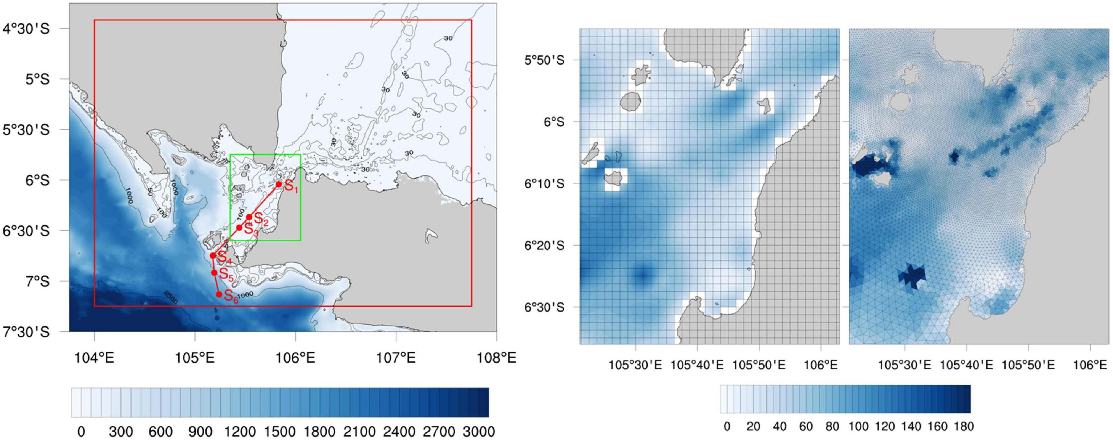
Figure 10. Left panel: Bathymetry contour map of the Sunda Strait experiment area as obtained from GEBCO datasets at a 30 Arc seconds resolution. Red rectangles delineate the boundaries of the nested domains. Red dots indicate the location of the ship-mounted ADCP station from 5AM (S1) to 11AM (S6). The green box highlights the subdomain region, where we zoom to highlight the structured and unstructured grid features (right panels). Right panels: Horizontal grids for the subdomain region implemented by the structured (left panel) and unstructured (right panel) grid SURF models. The resolution of the structured grid corresponds to about 2 km, while the unstructured grid resolution ranges from 100 m near the coast up to 3 km in the open sea.
Both structured and unstructured components of SURF were implemented in the Sunda Strait area (Figure 10) to analyze how the increased model resolution affects the realism of the ocean currents in the strait. The current model results were compared with the Shipboard ADCP current data extracted from the Global Ocean Current Database (GOCD6). The data refer to an along-track shipboard ADCP profile of between 20–400 m water depths near the Sunda Strait (red line in the left panel of Figure 10) collected on 4 December 1995, from 5:00 AM to 11:00 AM.
Model Set-up
Appendix Table A6 summarizes the values selected for the experiment, in terms of both the structured grid (left column) and unstructured grid (right column) components of SURF. Both models were implemented in the same domain (the red rectangle on the left panel of Figure 10), which is a 416 km longitude by 317 km latitude area, extending from 104E to 107.75E and from 7.25S to 4.41S. The initial and lateral boundary conditions for the nested models were extracted from the CMEMS-global reanalysis daily mean product (GLOBAL_REANALYSIS_ PHY_001_030). The CMEMS model was defined on a regular grid with a horizontal resolution of 1/12° (approx. 8 km) and 50 z-levels.
The structured grid SURF model domain consists of 181 × 137 grid points in the horizontal plane with a resolution of 1/48° (about 2300 m). The unstructured grid model was implemented in the domain with a horizontal resolution of 3 km in the open ocean, with local refinement of up to 100 m in the Sunda Strait. A proportion of the structured and unstructured horizontal mesh is shown on the right panel of Figure 10. On the vertical axis, SURF-S approximately doubles the vertical resolution of the parent model. The vertical grid consists of 100 z-levels with a stretching factor of hcr = 16 and a model level with a maximum stretching of hth = 50. The locations of the vertical levels were smoothly distributed from 0.5 m to a maximum depth of 2945 m and had level thicknesses that increased with depth from approximately 3 m to 90 m. The SURF-U z-layers are 101. The layer thicknesses are 2 m from the sea surface down to 110 m and then progressively (stepwise) increase toward the bottom with a maximum layer thickness of 100 m starting from 1000 m of depth.
Bathymetry was derived in both components from the GEBCO datasets with 30 arc-seconds (about 830 × 830 meters) (Becker et al., 2009) by linear interpolation of depth data into the SURF model grid. The tidal forcing was provided at the open boundaries in SURF-U and SURF-S, but SURF-S also includes the equilibrium tidal elevation. The eight most significant harmonic constituents (M2, S2, N2, K2, K1, O1, P1, and Q1) are considered.
The atmospheric fields are obtained from the European Center for Medium-Range Weather Forecasts ERA5 reanalysis fields (Hersbach et al., 2020), with a 1/8° horizontal resolution and 6-h frequency.
Results
A simulation over 5 days (30 November 1995 at 00:00 to 4 December 1995 at 24:00) was conducted using both SURF-S and SURF-U models. The first 4 days of the simulations were considered to be the spin-up time necessary for the downscaled model to produce dynamically adjusted fields after initialization from the coarser-resolution model.
Figure 11 displays the daily-averaged surface current fields for 4 December, as obtained from the SURF-S (middle panel), SURF-U, and CMEMS models (left panel). The dominant large-scale current pattern in the strait can be recognized across all solutions, but the current velocities in terms of amplitude in CMEMS are almost half those of both the SURF-U and SURF-S solutions. The SURF high-resolution simulations also show greater realism of the currents around the Sangiang island, which are missing in the CMEMS. As the Sangiang island is 6.5 km wide, the Glob-CMEMS with ∼10 km resolution clearly cannot adequately resolve the island-induced flow, but it is, however, capable of providing realistic initial and lateral boundary conditions.
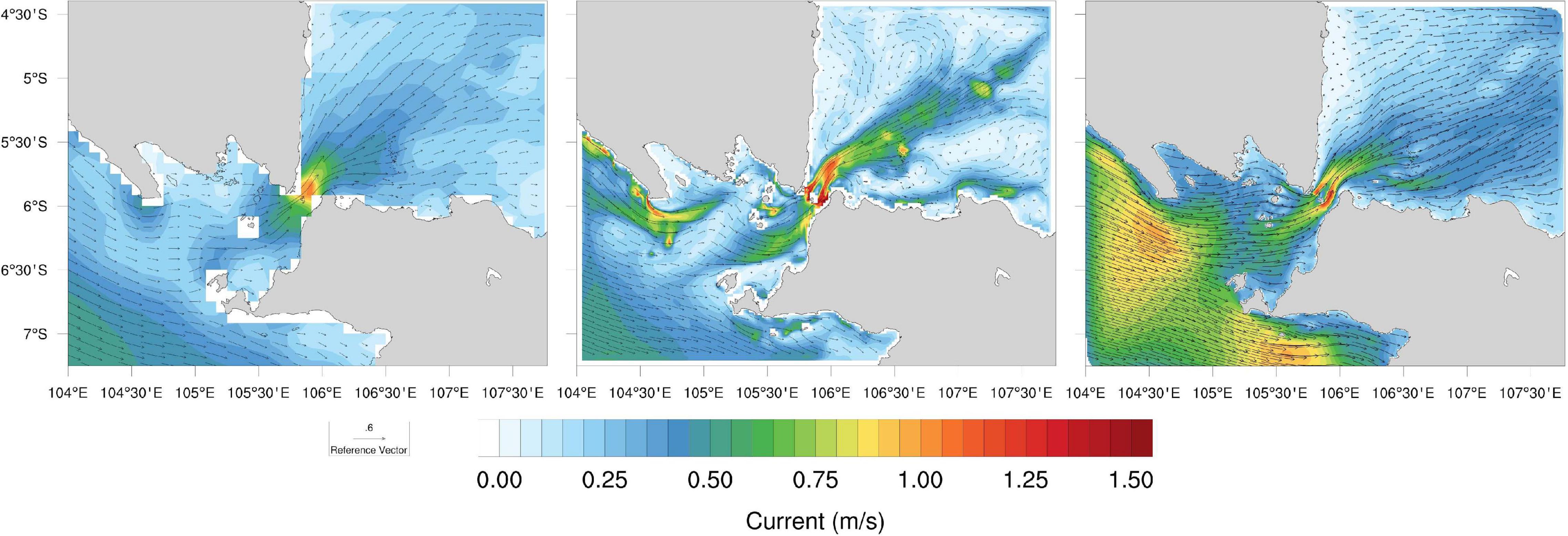
Figure 11. Averaged daily surface velocity fields on 4 December, 1995 of the parent CMEMS model (left panel), the structured (central panel), and unstructured (right panel) grid SURF model.
Scatter diagrams of the zonal and meridional components of the three model solutions are plotted in Figure 12 together with the number of points used and the regression coefficient. Each regression line is determined so that the sum of the distances between the line and each data point is minimized. All of the data of the six available ADCP stations are used in the figure. Both regression lines for zonal (left panel) and meridional (right panel) components, indicate that the ADCP and SURF model are well correlated. The correlation coefficient for the zonal velocity is 0.74 and 0.75 for SURF-S and SURF-U, respectively, showing a correlation improvement in the CMEMS with a coefficient of 0.42. Similar results are obtained for the meridional velocity component.
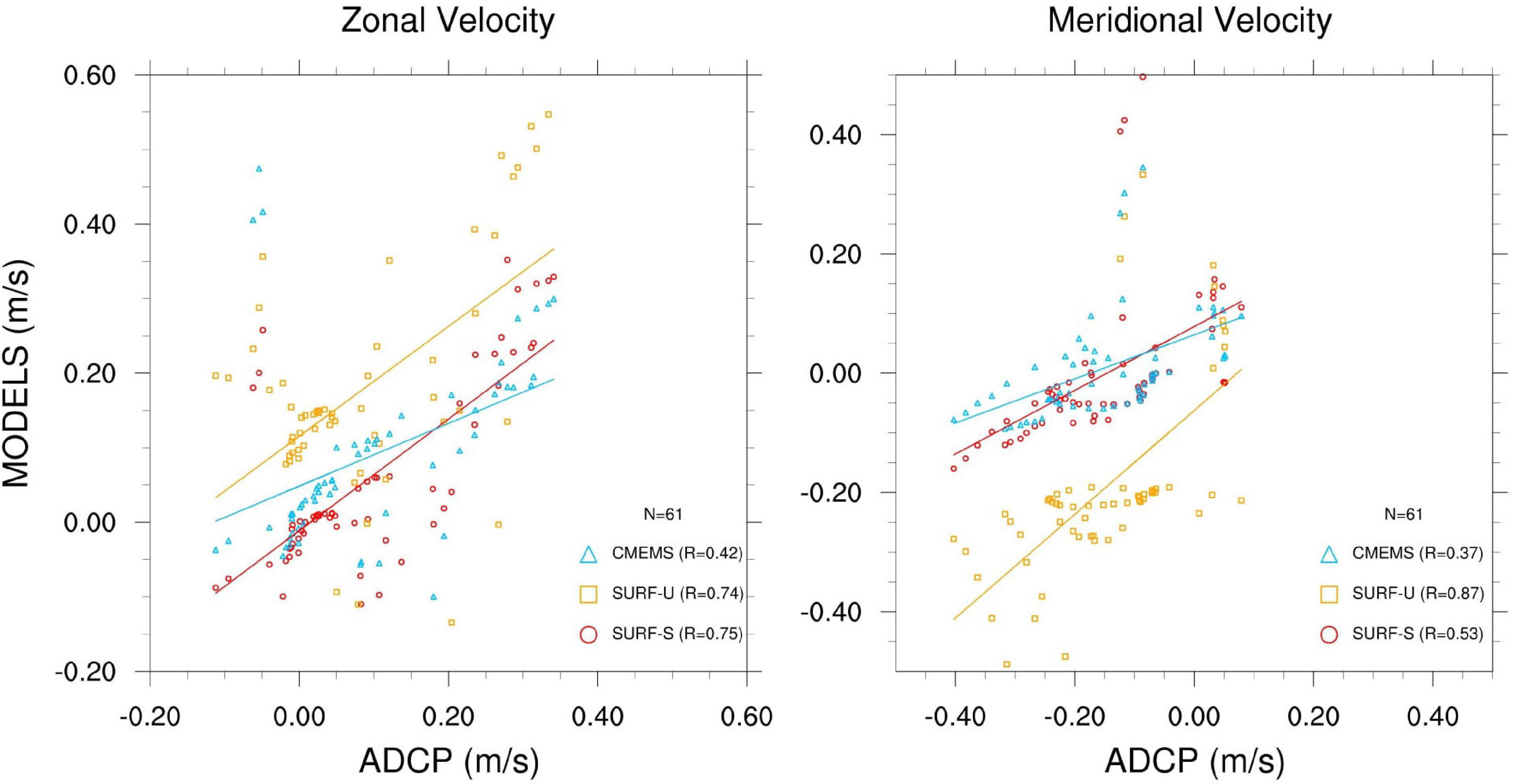
Figure 12. Scatter diagram of zonal (left panel) and meridional (right panel) components between the ADCP velocity and the structured SURF-S velocity (red circles), the unstructured SURF-U velocity (orange squares), and the CMEMS velocity (blue triangles). The regression for each model is indicated by the straight line. Numbers of data (N) used and correlation coefficients (R) are also shown in each panel.
Summary and Conclusion
In this paper, we present four different downscaling case studies using the CMEMS Global and Regional analyses and re-analyses for initial and lateral boundary conditions, using a new modeling platform, SURF, which contains both structured and unstructured numerical models. All interpolation and boundary condition issues are implemented in the platform, which is thus easily deployable in open ocean and coastal areas where resolution is required. The downscaled fields are then used in four coastal and near coastal areas to demonstrate the benefits of downscaling for the simulation of object drift, oil spill events, storm surges, and currents in narrow straits.
Downscaling allows not only to increase model resolution but also to include geometric features of the coastal areas that affect the flow field, the use of higher resolution bathymetry and the incorporation of more processes such as tides and specific parametrizations in the domain of interest. However, there are still many assumptions in the downscaling: the extrapolation (SOL) procedure used might be limiting the quality of the initial condition, the use of a simple forecast deterministic framework might limit the possibility to improve given the uncertainties associated with the small spatial and temporal scales.
In the first test case, we present the unstructured SURF component implementation in the Gulf of Taranto combined with a Lagrangian trajectory model, which is used to provide information to search and rescue operations. The SURF model results are compared with CTD, ADCP, tide-gauge data and drifter trajectories. The nested model is shown to provide improved results in terms of the parent hydrodynamics CMEMS fields. In terms of the application of this downscaled hydrodynamics to the drift of objects, SURF-U current field improves the drift half of the times and this might be due to higher frequency processes not considered such as the coupling with Stokes drift and high frequency atmospheric forcing.
In the second test case, we present the unstructured SURF model component implemented in the Azores Archipelago to study the storm surge impact of hurricane Lorenzo in October 2019. The SURF model results show an increase in sea level with respect to CMEMS in the area surrounding the two islands and it is argued that this is due to the downscaling to higher resolution and to the different wind stress formulation in the parent and nested models. The model results were compared with satellite altimetry, and a higher correlation of SURF-U simulations with CMEMS was found.
In the third test case, we presented a double-nested model experiment using the structured SURF model component combined with the oil spill model implemented in the offshore waters of the Spanish northwest coast, which is used to reproduce the oil spill drift associated with the Prestige accident. The flow field showed an intensified surface current speed and additional finer-scale motion emerging in the higher resolution SURF currents, which had better agreement with the satellite imagery. In particular, the second nesting, which went down to 500 m resolution in the offshore and near coastal areas, shows the oil arrival at the coast while the others did not in agreement with observations.
In the fourth test case, the structured and unstructured grid components were compared in the area of the Sunda Strait, to analyze how the model’s horizontal resolution influences the ocean surface currents. The dominant large-scale circulation in the Sunda Strait can be recognized in both the CMEMS and SURF solutions. However, additional features emerged at smaller scales permitted by the increased SURF grid resolution, and SURF improvements were documented for ADCP velocity recording in the area.
The game-changing paradigm described in this paper stems from the availability of large-scale, operational products for the past 20–30 years and daily forecasts. We demonstrate that the quality of the initial and lateral boundary condition fields in CMEMS products is high enough to initialize and force the boundaries of SURF. SURF downscaling augments the realism of the ocean hydrodynamics by adding geometry, resolution, tidal and atmospheric forcing. The high-resolution downscaling can in turn affect the quality of societal-impact models for oil spill forecasting, search and rescue, and the impact-based forecasting of storm surges in a fully baroclinic ocean circulation framework. We argue that this capacity is critical in supporting emergency response and DRR planning, which typically occur in very localized areas of the world’s oceans. We also suggest that in the future such relocatable models will allow climate change projections to be properly downscaled, and will probably require multiple nesting, as already implemented in the SURF platform.
Data Availability Statement
The raw data supporting the conclusions of this article will be made available by the authors, without undue reservation.
Author Contributions
FT, IF, and NP designed the research. FT and IF led the study, performed the research, data analysis, and produced the figures. NP fundamental helped in interpretation of modeling results and revising the work. SC helped to develop pre- and post-processing modeling tools. EJ helped understanding all aspects related to the Lagrangian drift model. DI, SM, and GC helped revising the work. All authors contributed to the article and approved the submitted version.
Funding
Support for this work was provided by the IMMERSE (No. 821926, funded by the European Commission under the H2020 Programme) and Strategic project #4 “A multihazard prediction and analysis testbed for the global coastal ocean” of CMCC. Partial funding through the IMPRESSIVE (No. 821922, funded by H2020 Programme), SAGAcE (funded by Apulia Region, Italy, No. M7 × 3HL2), and EUROSEA (No. 862626, funded by H2020 Programme) projects are gratefully acknowledged.
Conflict of Interest
The authors declare that the research was conducted in the absence of any commercial or financial relationships that could be construed as a potential conflict of interest.
Acknowledgments
The authors wish to thank Vladyslav Lyubartsev and Augusto A. Sepp Neves (CMCC, Italy) for their collaboration and support.
Footnotes
- ^ https://www.surf-platform.org/
- ^ http://gmsh.info/
- ^ https://www.blender.org/
- ^ https://www.emodnet-bathymetry.eu/
- ^ https://www.gebco.net/
- ^ https://www.ncei.noaa.gov/products/global-ocean-currents-database-gocd
References
Albaigés, J., Morales-Nin, B., and Vilas, F. (2006). The Prestige oil spill: a scientific response. Mar. Pollut. Bull. 53, 205–207. doi: 10.1016/j.marpolbul.2006.03.012
Arakawa, A., and Lamb, V. R. (1981). A potential energy and enstrophy conserving scheme for the shallow water equations. Mont. Weather Rev. 109, 18–36. doi: 10.1175/1520-0493(1981)109<0018:apeaec>2.0.co;2
Balseiro, C. F., Carracedo, P., Gómez, B., Leitão, P. C., Montero, P., Naranjo, L., et al. (2003). Tracking the prestige oil spill: an operational experience in simulation at MeteoGalicia. Weather 58, 452–458. doi: 10.1002/wea.6080581204
Barnier, B., Madec, G., Penduff, T., Molines, J. M., Treguier, A. M., le Sommer, J., et al. (2006). Impact of partial steps and momentum advection schemes in a global circulation model at eddy permitting resolution. Ocean Dyn. 56, 543–567. doi: 10.1007/s10236-006-0082-1
Becker, J. J., Sandwell, D. T., Smith, W. H. F., Braud, J., Binder, B., Depner, J., et al. (2009). Global bathymetry and elevation data at 30 arc seconds resolution: SRTM30_PLUS. Mar. Geod. 32, 355–371. doi: 10.1080/01490410903297766
Booij, N., Ris, R. C., and Holthuijsen, L. H. (1999). A third generation wave model for coastal regions, part 1: model description and validation. J. Geophys. Res. 104, 7649–7666. doi: 10.1029/98jc02622
Burchard, H., and Petersen, O. (1999). Models of turbulence in the marine environment a comparative study of two equation turbulence models. J. Mar. Syst. 21, 29–53. doi: 10.1016/s0924-7963(99)00004-4
Calkins, J. (2015). Moving forward after sendai: how countries want to use science, evidence and technology for disaster risk reduction. PLoS Curr. Disasters 7. doi: 10.1371/currents.dis.22247d6293d4109d09794890bcda1878
Carabine, E. (2015). Revitalizing evidence-based policy for the sendai framework for disaster risk reduction 2015–2030: lessons from existing international science partnerships. PLoS Curr. Disasters 7. doi: 10.1371/currents.dis.aaab45b2b4106307ae2168a485e03b8a
Carracedo, P., Torres-LoLpez, S., Barreiro, M., Montero, P., Balseiro, C. F., Penabad, E., et al. (2006). Improvement of pollutant drift forecast system applied to the prestige oil spills in Galicia Coast (NW of Spain): development of an operational system. Mar. Pollut. Bull. 53, 350–360. doi: 10.1016/j.marpolbul.2005.11.014
Clementi, E., Pistoia, J., Escudier, R., Delrosso, D., Drudi, M., Grandi, A., et al. (2019). Mediterranean Sea Analysis and Forecast (CMEMS MED-Currents, EAS5 system). Copernicus Monitoring Environment Marine Service (CMEMS). doi: 10.25423/CMCC/MEDSEA_ANALYSIS_FORECAST_PHY_006_013_EAS5
Cressman, G. P. (1959). An operational objective analysis system. Mon. Weather Rev. 87, 367–374. doi: 10.1175/1520-0493(1959)087<0367:aooas>2.0.co;2
De Dominicis, M., Falchetti, S., Trotta, F., Pinardi, N., Giacomelli, L., Napolitano, E., et al. (2014). A relocatable ocean model in support of environmental emergencies. Ocean Dyn. 64, 667–688. doi: 10.1007/s10236-014-0705-x
De Dominicis, M., Pinardi, N., Zodiatis, G., and Lardner, R. (2013). MEDSLIK-II, a Lagrangian marine surface oil spill model for short-termforecasting—part 1: theory. Geosci. Model Dev. 6, 1851–1869. doi: 10.5194/gmd-6-1851-2013
De Pascalis, F., Petrizzo, A., Ghezzo, M., Lorenzetti, G., Manfé, G., Alabiso, G., et al. (2015). Estuarine circulation in the Taranto Seas, integrated environmental characterization of the contaminated marine coastal area of Taranto, Ionian Sea (southern Italy), the RITMARE Project. Environ. Sci. Pollut. R. 23, 12515–12534.
Egbert, G. D., and Erofeeva, S. Y. (2002). Efficient inverse modeling of barotropic ocean tides. J. Atmos. Ocean. Technol. 19, 183–204. doi: 10.1175/1520-0426(2002)019<0183:eimobo>2.0.co;2
Engerdahl, H. (1995). Use of the flow relaxation scheme in a three-dimensional baroclinic ocean model with realistic topography. Tellus A 47, 365–382. doi: 10.1034/j.1600-0870.1995.t01-2-00006.x
Ezer, T. (2019). Numerical modeling of the impact of hurricanes on ocean dynamics: sensitivity of the Gulf Stream response to storm’s track. Ocean Dyn. 69, 1053–1066. doi: 10.1007/s10236-019-01289-9
Federico, I., Pinardi, N., Coppini, G., Oddo, P., Lecci, R., and Mossa, M. (2017). Coastal ocean forecasting with an unstructured grid model in the southern Adriatic and northern Ionian seas. Nat. Hazards Earth Syst. Sci. 17, 45–59. doi: 10.5194/nhess-17-45-2017
Federico, I. N., Pinardi, V., Lyubartsev, F., Maicu, S., Causio, F., Trotta, C., et al. (2020). Observational evidence of the basin-wide gyre reversal in the Gulf of Taranto. Geophys. Res. Lett. 47:e2020GL091030.
Ferrarin, C., Maicu, F., and Umgiesser, G. (2017). The effect of lagoons on Adriatic Sea tidal dynamics. Ocean Model. 119, 57–71. doi: 10.1016/j.ocemod.2017.09.009
Haley, P. J. Jr., and Lermusiaux, P. F. J. (2010). Multiscale two-way embedding schemes for free-surface primitive equations in the “multidisciplinary simulation, estimation and assimilation system. Ocean Dyn. 60, 1497–1537. doi: 10.1007/s10236-010-0349-4
Hellermann, S., and Rosenstein, M. (1983). Normal wind stress over the world ocean with error estimates. J. Phys. Oceanogr. 13, 1093–1104. doi: 10.1175/1520-0485(1983)013<1093:nmwsot>2.0.co;2
Hersbach, H., Bell, B., Berrisford, P., Hirahara, S., Horányi, A., Muñoz-Sabater, J., et al. (2020). The ERA5 global reanalysis. Q. J. R. Meteorol. Soc. 146, 1999–2049.
Jackett, D. R., and Mcdougall, T. J. (1995). Minimal adjustment of hydrographic profiles to achieve static stability. J. Atmos. Ocean.Technol. 12, 381–389. doi: 10.1175/1520-0426(1995)012<0381:maohpt>2.0.co;2
Jansen, E., Coppini, G., and Pinardi, N. (2016). Drift simulation of MH370 debris using superensemble techniques. Nat. Hazards Earth Syst. Sci. 16, 1623–1628. doi: 10.5194/nhess-16-1623-2016
Lermusiaux, P. F. J. (2007). “Adaptive modeling, adaptive data assimilation and adaptive sampling,” in Refereed Invited Manuscript. Special Issue on “Mathematical Issues and Challenges in Data Assimilation for Geophysical Systems: Interdisciplinary Perspectives”, Vol. 230, eds C. K. R. T. Jones and K. Ide (Physica D), 172–196. doi: 10.1016/j.physd.2007.02.014
Le Traon, P. Y., Reppucci, A., Reppucci, A., Fanjul, E. A., Aouf, L., Behrens, A., et al. (2019). From Observation to Information and Users: the Copernicus Marine Service Perspective. Front. Mar. Sci. 6:234. doi: 10.3389/fmars.2019.00234
Lermusiaux, P. F. J., Haley, P. J. Jr., Jana, S., Gupta, A., Kulkarni, C. S., Mirabito, C., et al. (2017). Optimal planning and sampling predictions for autonomous and lagrangian platforms and sensors in the Northern Arabian Sea. Oceanography 30, 172–185. doi: 10.5670/oceanog.2017.242
Lermusiaux, P. F. J., Haley, P. J. Jr., Leslie, W. G., Agarwal, A., Logutov, O., and Burton, L. J. (2011). Multiscale physical and biological dynamics in the Philippines Archipelago: predictions and Processes. Oceangraphy. Phil. Ex. Issue 24, 70–89. doi: 10.5670/oceanog.2011.05
Luettich, R. A., and Westerink, J. J. (2004). Formulation and numerical implementation of the 2D/3D ADCIRC Finite Element Model Version 44.XX. Theory Report. Available online at: https://adcirc.org/wp-content/uploads/sites/2255/2018/11/adcirc_theory_2004_12_08.pdf (accessed August 12, 2004).
Madec, G. (2008). NEMO Ocean Engine, Note du Pole de Modelisation. France: Institut Pierre-Simone Laplace (IPSL), 27.
Madec, G. (2016). NEMO reference manual 3_6_STABLE: “NEMO Ocean Engine” Note du Pôle de Modélisation. France: Institut Pierre-Simon Laplace (IPSL). No 27 ISSN No 1288-1619.
Martin, P. (2000). Description of the Navy Coastal Ocean Model Version 1.0. NRL report NRL/FR/7322-00-9961. Stennis Space Center, MS: Naval Research Laboratory.
Oddo, P., and Pinardi, N. (2008). Lateral open boundary conditions for nested limited area models: a process selective approach. Ocean Model. 20, 134–156. doi: 10.1016/j.ocemod.2007.08.001
Oliveira, A., Fortunato, A. B., Rogeiro, J., Teixeira, J., Azevedo, A., Lauvaud, L., et al. (2020). OPENCoastS: an open-access service for the automatic generation of coastal forecast systems. Environ. Model. Softw. 124:104585. doi: 10.1016/j.envsoft.2019.104585
Onken, R. (2017). Forecast skill score assessment of a relocatable ocean prediction system, using a simplified objective analysis method. Ocean Sci. 13, 925–945. doi: 10.5194/os-13-925-2017
Pacanowski, R. C., and Philander, S. G. H. (1981). Parameterisation of vertical mixing in numerical models of tropical oceans. J. Phys. Oceanogr. 11, 1443–1451. doi: 10.1175/1520-0485(1981)011<1443:povmin>2.0.co;2
Pettenuzzo, D., Large, W. G., and Pinardi, N. (2010). On the corrections of ERA-40 surface flux products consistent with the Mediterranean heat and water budgets and the connection between basin surface total heat flux and NAO. J. Geophys. Res. 115:C06022.
Pinardi, N., Allen, I., Demirov, E., De Mey, P., Korres, G., Lascaratos, A., et al. (2003). The Mediterranean ocean Forecasting System: first phase of implementation (1998-2001). Ann. Geophys. 21, 3–20. doi: 10.5194/angeo-21-3-2003
Pinardi, N., Cavaleri, L., Coppini, G., Mey, P., Fratianni, C., Huthnance, J., et al. (2017). From weather to ocean predictions: an historical viewpoint. J. Mar. Res. 75, 103–159. doi: 10.1357/002224017821836789
Pinardi, N., Lyubartsev, V., Cardellicchio, N., Caporale, C., Ciliberti, S., Coppini, G., et al. (2016). Marine rapid environmental assessment in the gulf of taranto: a multiscale approach. Nat. Hazards Earth Syst. Sci. 16, 2623–2639. doi: 10.5194/nhess-16-2623-2016
Robinson, A. (1999). Forecasting and simulating coastal ocean processes and variabilities with the Harvard Ocean Prediction System. Coastal Ocean Prediction, AGU Coastal and Estuarine Studies Series. Am. Geophys. Union 20, 77–100.
Robinson, A. R., Carton, J. A., Pinardi, N., and Mooers, C. N. K. (1986). Dynamical forecasting and dynamical interpolation: an experiment in the California current system. J. Phys. Oceanogr. 16, 1561–1579. doi: 10.1175/1520-0485(1986)016<1561:DFADIA>2.0.CO;2
Shchepetkin, A. F., and McWilliams, J. C. (2003). A method for computing horizontal pressure-gradient force in an oceanic model with a nonaligned vertical coordinate. J. Geophys. Res. 108:3090. doi: 10.1029/2001JC001047
Shchepetkin, A. F., and McWilliams, J. C. (2005). The regional ocean modeling system: a split-explicit, free-surface, topography following coordinates ocean model. Ocean Model. 9, 347–404. doi: 10.1016/j.ocemod.2004.08.002
Smagorinsky, J. (1963). General circulation experiments with the primitive equations. Mont. Weather Rev. 91, 99–164. doi: 10.1175/1520-0493(1963)091<0099:gcewtp>2.3.co;2
Thomalla, F., Downing, T., Spanger-Siegfried, E., Han, G., and Rockström, J. (2006). Reducing hazard vulnerability: towards a common approach between disaster risk reduction and climate adaptation. Disasters 30, 39–48. doi: 10.1111/j.1467-9523.2006.00305.x
Trotta, F., Fenu, E., Pinardi, N., Bruciaferri, D., Giacomelli, L., Federico, I., et al. (2016). A Structured and unstructured grid relocatable ocean platform for forecasting (SURF). Deep Sea Res. II 113, 54–75. doi: 10.1016/j.dsr2.2016.05.004
Trotta, F., Pinardi, N., Fenu, E., Grandi, A., and Lyubartsev, V. (2017). Multi-nest high-resolution model of submesoscale circulation features in the Gulf of Taranto. Ocean Dyn. 67, 1609–1625. doi: 10.1007/s10236-017-1110-z
Umgiesser, G., Melaku Canu, D., Cucco, A., and Solidoro, C. (2004). A finite element model for the Venice Lagoon. Development, set up, calibration and validation. J. Mar. Syst. 51, 123–145. doi: 10.1016/j.jmarsys.2004.05.009
Verri, G., Pinardi, N., Oddo, P., Ciliberti, S. A., and Coppini, G. (2018). River runoff influences on the central mediterranean overturning circulation. Clim. Dyn. 50, 1675–1703. doi: 10.1007/s00382-017-3715-9
Vieira, G. S., Rypina, I. I., and Allshouse, M. R. (2020). Uncertainty quantification of trajectory clustering applied to ocean ensemble forecasts. Fluids 2020:184. doi: 10.3390/fluids5040184
Zelinsky, D. A. (2019). Hurricane Lorenzo. National Hurricane Center Tropical Cyclone Report. Available online at: https://www.nhc.noaa.gov/data/tcr/AL132019_Lorenzo.pdf) (accessed December 16, 2019).
APPENDIX A: Model Parameters
This appendix contains the list of tables and the model parameters and the values used in the four downstream case studies. Appendix Table A1 lists the model user-parameters for both the structured and unstructured SURF model components. Appendix Table A2 summarizes the values chosen for the Gulf of Taranto case study (Section “Case Study 1: Drifter Trajectories in the Taranto Seas”), Appendix Table A3 those chosen for the Azores Archipelago case study (Section “Case Study 2: Storm Surges in the Azores Archipelago”) and Appendix Table A4 those chosen for the Prestige accident case study (Section “Case Study 3: The Prestige Oil Spill Accident in the Galicia Coast”). Appendix Table A5 list the model user-parameters for the Medslik-II oil spill model. Appendix Table A6 summarizes the values chosen for the Sunda Strait case study (Section “Case Study 4: The Sunda Strait”).
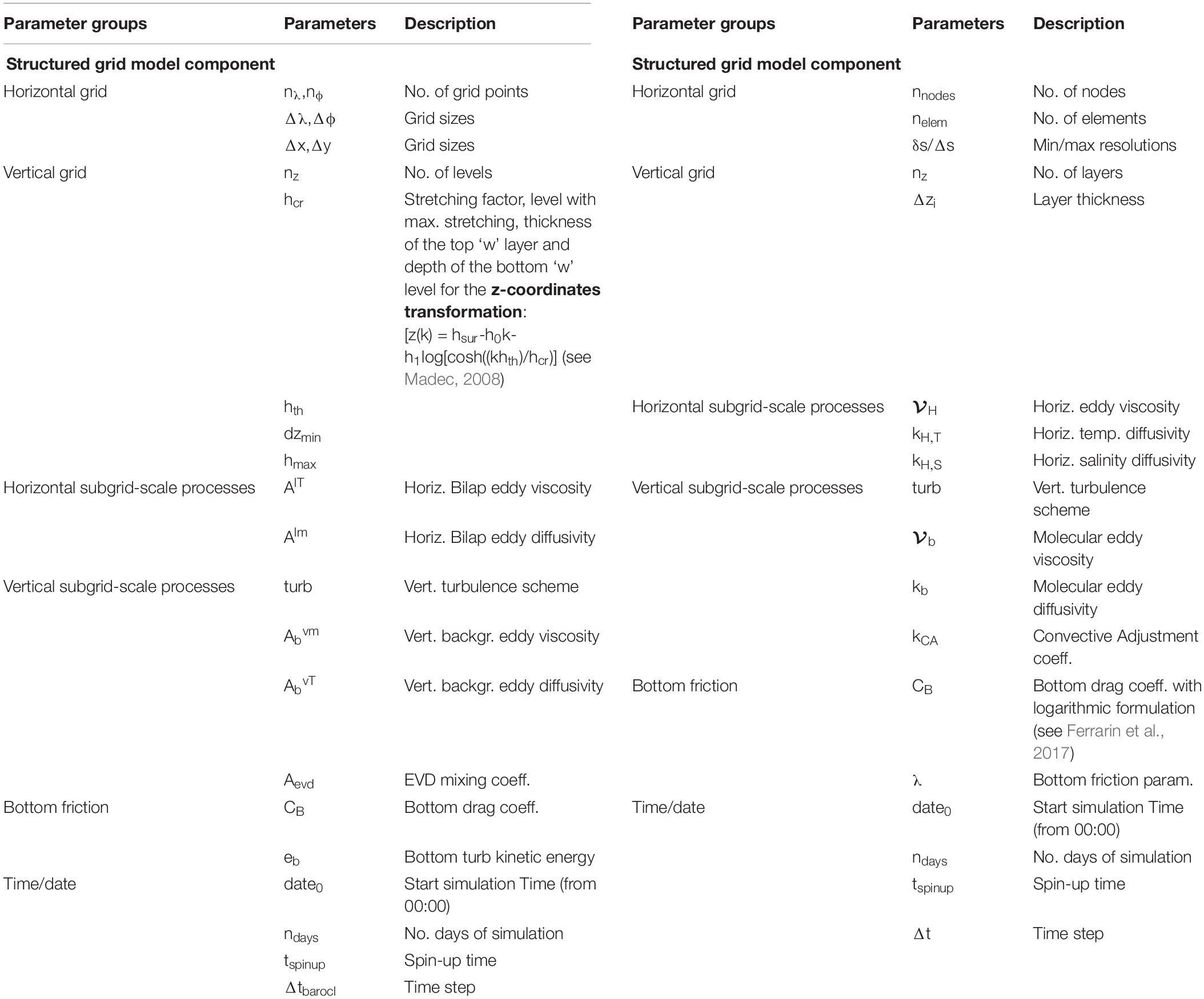
TABLE A1. Model user-parameters: (left) structured grid model component, (right) unstructured grid model component.
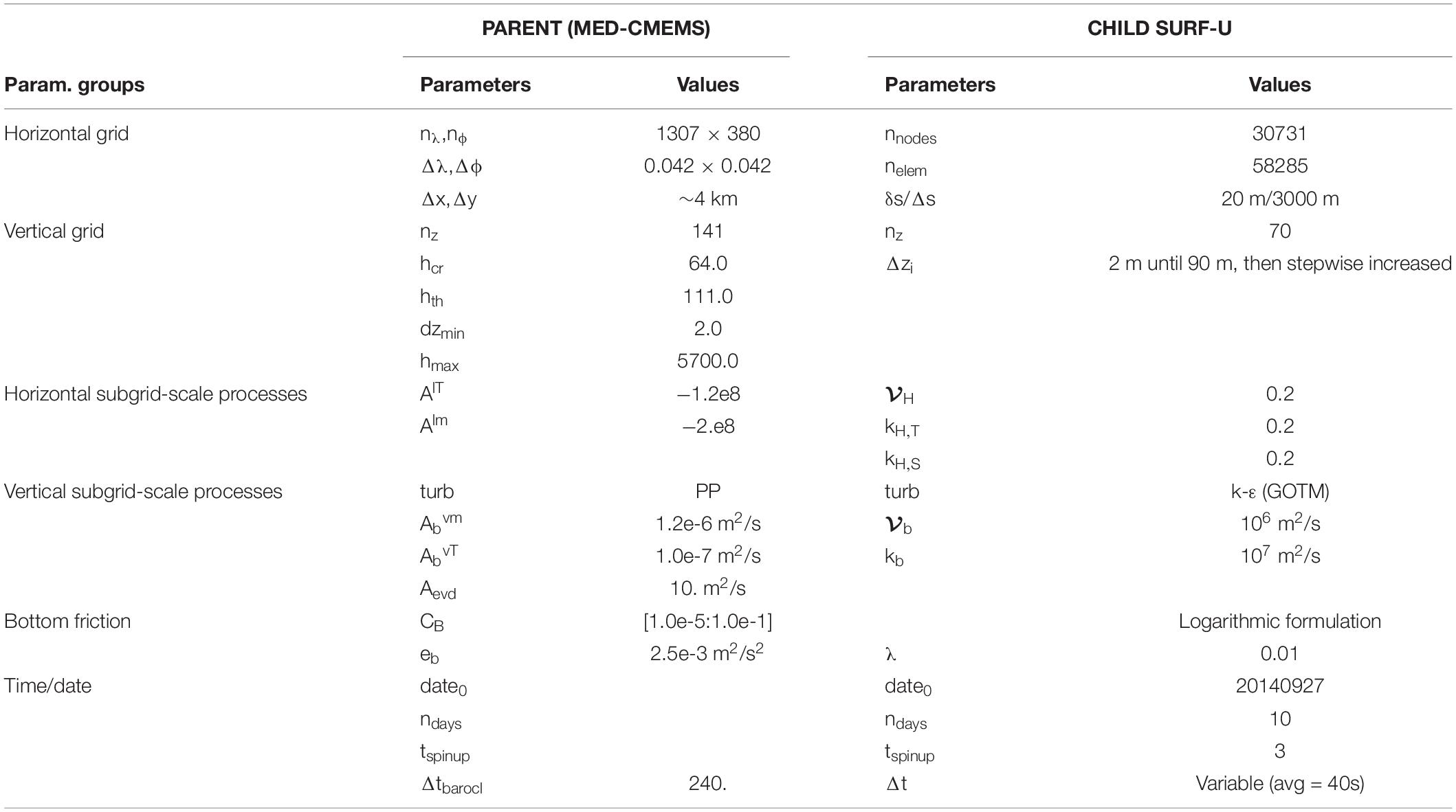
TABLE A2. Model parameters characterizing the Gulf of Taranto study case.
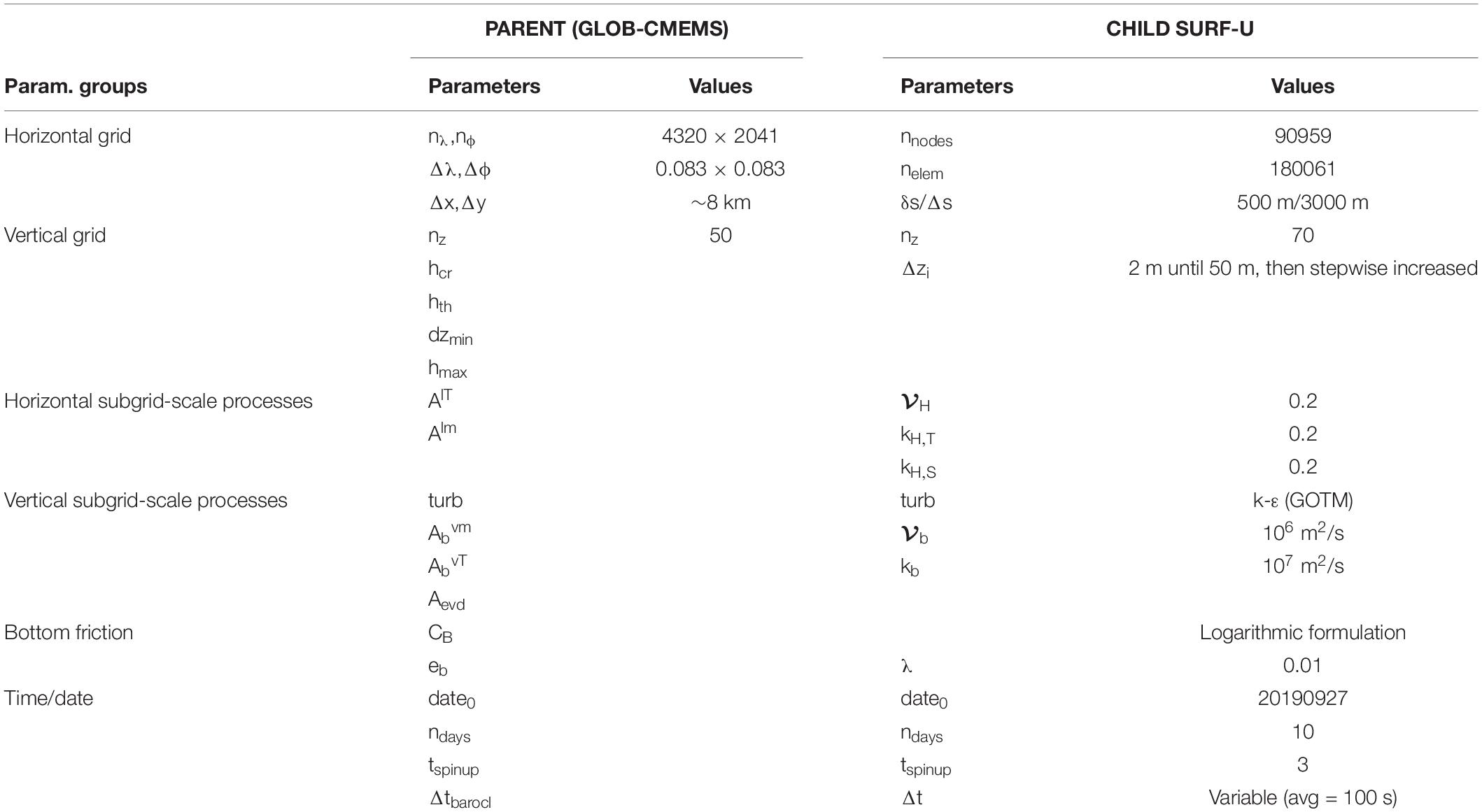
TABLE A3. Model parameters characterizing the Azores Archipelago study case.
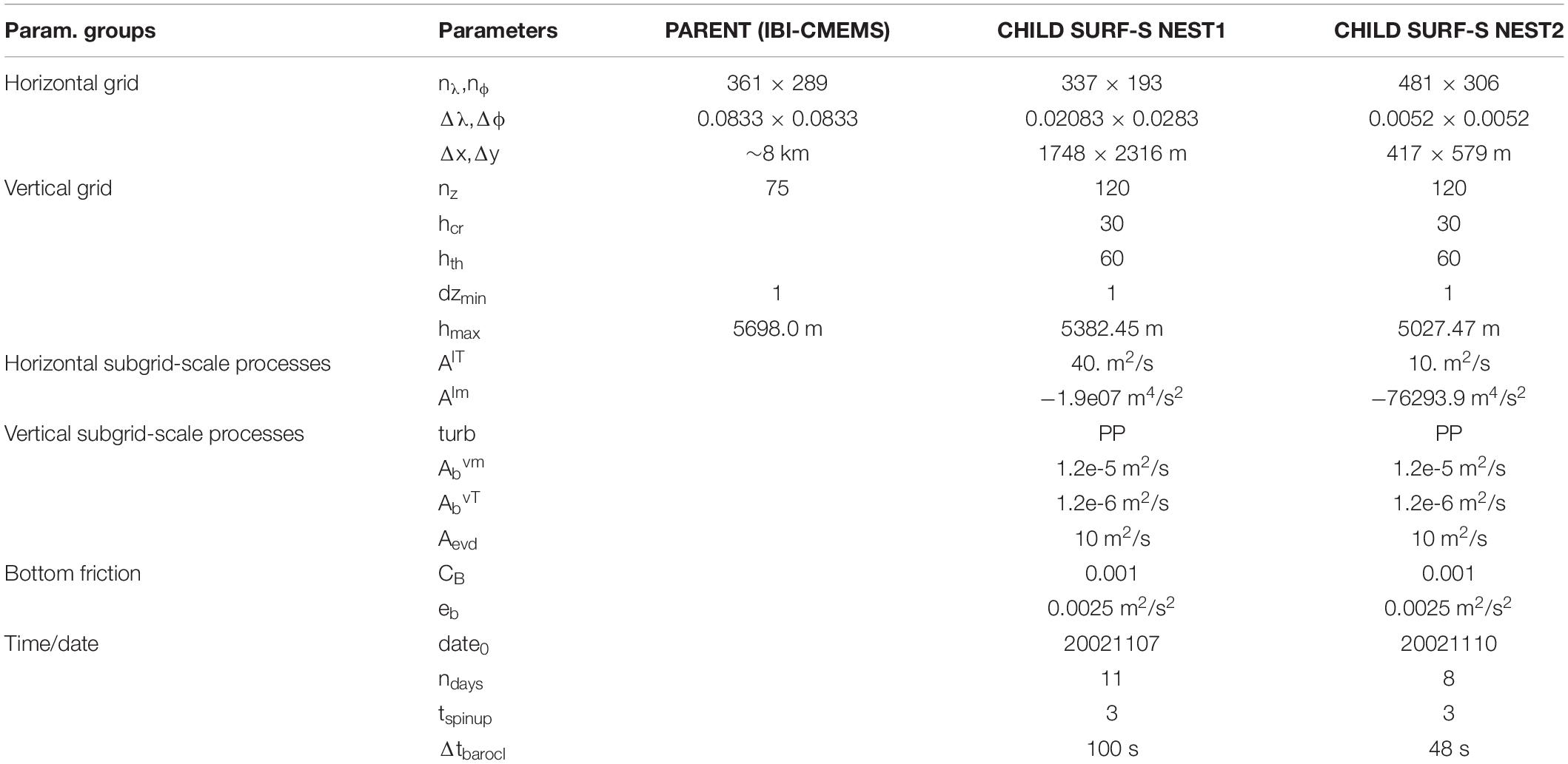
TABLE A4. Model parameters characterizing the Prestige accident study case.
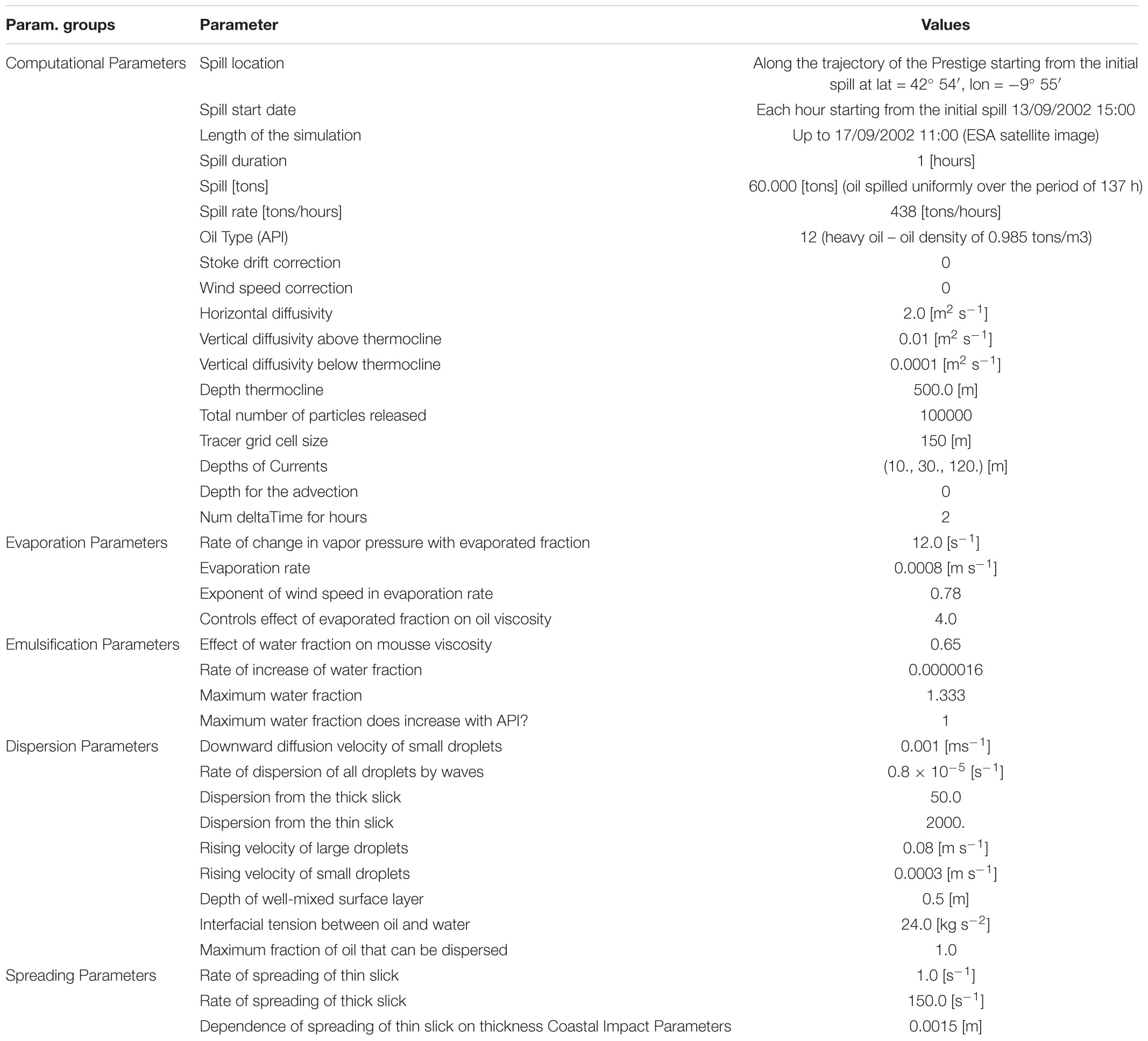
TABLE A5. Medslik-II model parameters for the Prestige accident experiment.
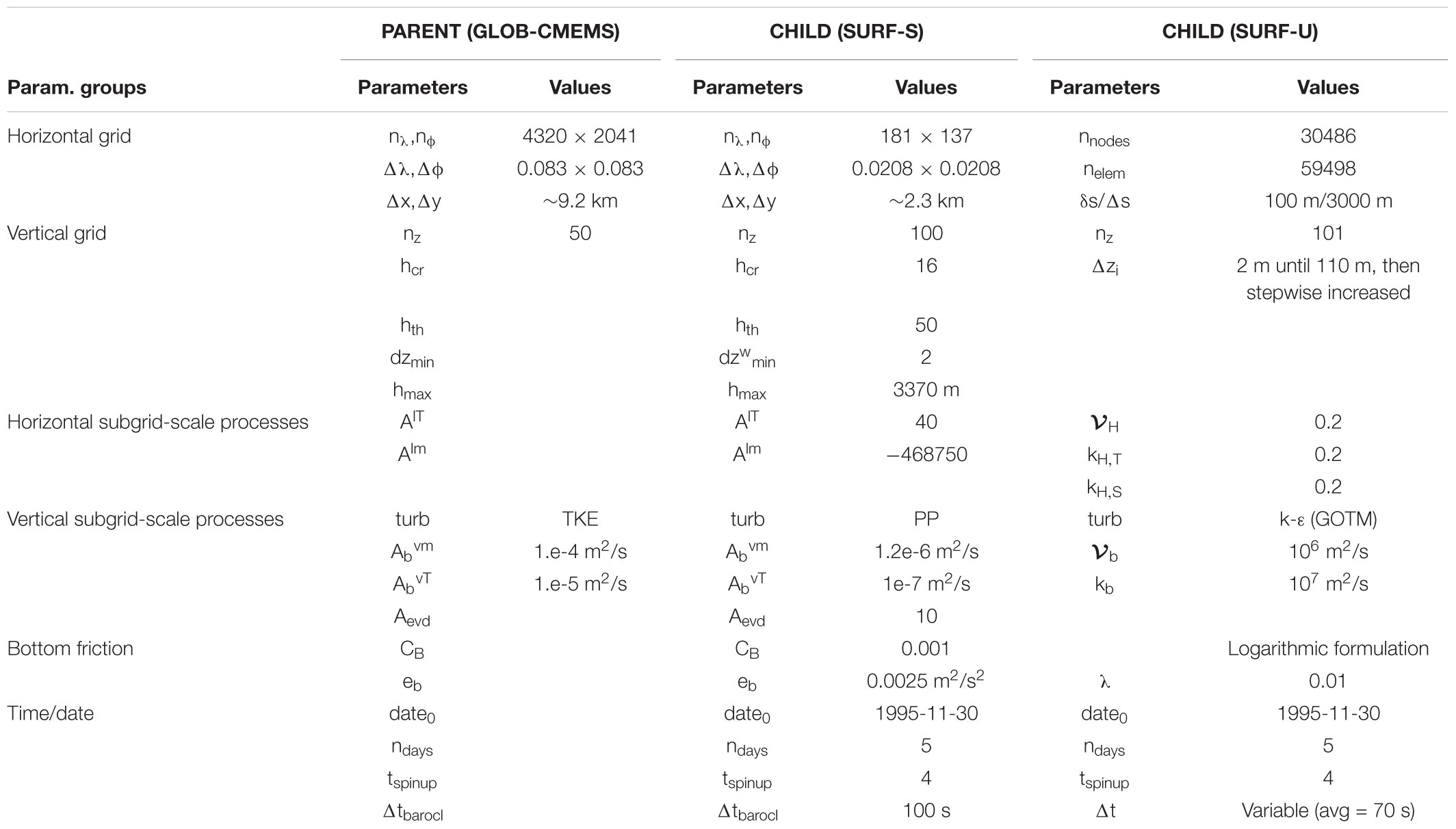
TABLE A6. Model parameters characterizing the Sunda Strait experiment setting.
Keywords: numerical modeling, ocean model, relocatable model, dynamical downscaling, multi-nesting method, high-resolution models, nested grid, structured and unstructured grid
Citation: Trotta F, Federico I, Pinardi N, Coppini G, Causio S, Jansen E, Iovino D and Masina S (2021) A Relocatable Ocean Modeling Platform for Downscaling to Shelf-Coastal Areas to Support Disaster Risk Reduction. Front. Mar. Sci. 8:642815. doi: 10.3389/fmars.2021.642815
Received: 16 December 2020; Accepted: 11 March 2021;
Published: 30 March 2021.
Edited by:
Joanna Staneva, Helmholtz Centre for Materials and Coastal Research (HZG), GermanyReviewed by:
Johannes Pein, Helmholtz Centre for Materials and Coastal Research (HZG), GermanyPaula Camus, University of Southampton, United Kingdom
Copyright © 2021 Trotta, Federico, Pinardi, Coppini, Causio, Jansen, Iovino and Masina. This is an open-access article distributed under the terms of the Creative Commons Attribution License (CC BY). The use, distribution or reproduction in other forums is permitted, provided the original author(s) and the copyright owner(s) are credited and that the original publication in this journal is cited, in accordance with accepted academic practice. No use, distribution or reproduction is permitted which does not comply with these terms.
*Correspondence: Francesco Trotta, francesco.trotta4@unibo.it