Estimating Cetacean Bycatch From Non-representative Samples (I): A Simulation Study With Regularized Multilevel Regression and Post-stratification

1. Introduction

Bycatch, the non-intentional capture or killing of non-target species in commercial or recreational fisheries, is a world wide threat to protected, endangered or threatened species (PETS) of marine megafauna (Gray and Kennelly, 2018), including seabirds (Martin et al., 2019), elasmobranchs (Pacoureau et al., 2021) and cetaceans (Avila et al., 2018). Bycatch in fishing gears, such as gillnets, is currently driving some small cetacean species to extinction (Brownell et al., 2019; Jaramillo-Legorreta et al., 2019). The European Commission recently issued infringement procedures against several Members States for failing to correctly transpose some provisions of European environmental law (the Habitats Directive, Council Directive 92/43/EEC), in particular the obligations related to the establishment of a coherent monitoring scheme of cetacean bycatch¹. The Data Collection Framework (DCF) provides a common framework in the European Union (EU) to collect, manage, and share data within the fisheries sector (Anonymous, 2019a). The Framework indicates that the Commission shall establish a Multi-Annual Union Programme (EU-MAP) for the collection and management of fisheries data which should be inclusive of data that allows the assessment of fisheries' impact on marine ecosystems. With respect to PETS (including cetaceans), the collection of high quality data usually requires a dedicated sampling scheme and methodology, and is generally different from those applied under the DCF (Stransky and Sala, 2019): “EU MAP remains not well-suited for the dedicated monitoring of rare and protected bycatch in high-risk fisheries since its main focus is the statistically-sound random sampling of all commercial fisheries (Ulrich and Doerner, 2021, p. 126).” In practice, the introduction of any programme on PETS bycatch under the DCF may be met with caution because of its perceived potential to disrupt data collection for fisheries management (Stransky and Sala, 2019). This perception implicitly relegates PETS bycatch as a side issue for fishery management rather than an integral part of it. It may explain the usually poor quality of bycatch data on PETS (ICES, 2020a).

Recent EU legislation (Regulation 2019/1241), referred to as the Technical Measures Regulation (TMR), requires Members States to collect scientific data on cetacean bycatch for the following métiers: pelagic trawls (single and pair), bottom-set gillnets and entangling nets; and high-opening trawls (Anonymous, 2019b). Unlike its predecessor (Council Regulation EC No. 812/2004), this Regulation does not require the establishment of dedicated observer schemes for cetacean bycatch data collection (Dolman et al., 2020). Furthermore, only vessels of an overall length of 15 m or more are to be monitored, but these represent a small fraction of the European fleet (less than 10% in 2019)². This vessel length criterion introduces bias in the bycatch monitoring data as the sample of vessels larger than 15 m is almost certainly dissimilar to smaller vessels. Even within the sample of vessels that are monitored, pragmatic considerations can complicate sampling. For example, in the United States, observer sampling trips are allocated first by region, port, and month, then randomly to vessels of particular categories within those monthly and spatial strata (ICES, 2009). Random allocation of observers to vessels follows sound statistical methodology and increases the likelihood of collecting unbiased data (Babcock and Pikitch, 2003). In France, observer days are allocated by port and by month for each fishery, but the exact vessel allocation is then negotiated and left at the discretion of skippers (ICES, 2009). Allocation is no longer random as skippers may only accept observers when cetacean bycatch risk is low (Benoît and Allard, 2009). Non-random allocation means potential bias in the collected data for monitoring bycatch as the sub-sample of skippers accepting an observer may be very different from skippers refusing to do so (Babcock and Pikitch, 2003).

One pragmatic solution bypassing observers is to mandate skippers to self-declare the non-intentional capture or killing of any PETS, as already required under the DCF (Anonymous, 2019a). In France, a national law from 2011 mandate fisheries to declare (without fear of prosecution) the bycatch of any cetacean species, but this law remained largely unknown to French fishermen until late 2019 (Cloâtre, 2020). In general, self-reported PETS bycatch data are sub-optimal as they may be heavily biased, non-representative (ICES, 2009) and typically provide poor information on which to base management decisions (National Marine Fisheries Service, 2004). Once again, the set of skippers who choose to declare bycatch may differ markedly from those who do not: for example the former take the extra time required to fill logbooks and thus provide accurate data while the latter do not. If this behavior is correlated to other attributes, e.g., a more acute awareness of threats to PETS resulting in practices that tend to minimize impact on PETS, data collected from skippers reporting bycatch would not be representative. There may also be an element of skippers genuinely forgetting to log PETS bycatch in the bustle of the fishing operation but this is random and unlikely to introduce bias. In addition, ground-truthing, for example with remote-electronic monitoring (REM; Course et al., 2020), would be required in order to ensure the quality and accuracy of self-reported data before their statistical analyses.

Another hurdle, of the statistical kind, with cetacean bycatch is the low frequency of these events. Assuming that implementing a representative sampling program were feasible, if bycatch is a rare event (Komoroske and Lewison, 2015), then few events would be observed for realistic sampling effort (Babcock and Pikitch, 2003; ICES, 2009). This paucity of observed event means a large uncertainty in statistical estimates: with a bycatch rate of the order of 0.01 event per fishing operation, a sample size of 1,100 observed operations would be required to obtain, in the best case scenario (no bias, statistical independence, etc.), the US recommended coefficient of variation of 30% (National Marine Fisheries Service, 2005, 2016; ICES, 2009; Carretta and Moore, 2014). The amount of observer coverage needed to reach this precision depends on fishery size and trip duration (Babcock and Pikitch, 2003). In practice, the sampling error depends on the overall design of the survey, of which the sample size is only one factor: for example a larger sample size could be needed if there are large “skipper-effects” as the same vessels would contribute fishing operations, and these would not be statistically independent. With a small sample size, uncertainty may be so large as to prevent using estimates altogether, even if one were to assume no bias in the data (Babcock and Pikitch, 2003). Given this challenge and the lack of uptake of dedicated monitoring programmes of cetacean bycatch in Europe over the last decade or more (Sala et al., 2019), it would appear prudent to seek methods of analysis that can handle the few and non-representative data available to robustly estimate bycatch rates.

The problem of having non-representative samples to carry out statistical analyses is ancient (Hansen and Hurwitz, 1946) and widespread: it pops up in many applied disciplines, including election forecasting (Wang et al., 2015; Kiewiet De Jonge et al., 2018), political sciences (Lax and Phillips, 2009; Zahorski, 2020), social sciences (Halsny, 2020), addiction studies (Rhem et al., 2020) or epidemiology (Zhang et al., 2014; Downes et al., 2018). In these disciplines, there are also intrinsic limits on improving the representativeness of sampling. For example, in polling, non-response rates can be above 90% (Forsberg, 2020). In other cases, some populations of interest may be hard to reach (Rhem et al., 2020), or answers may not be honest (St. John et al., 2014). Challenges lie in the accurate estimation of quantities of scientific interest (e.g., the true magnitude of bycatch in a fishery; Babcock and Pikitch, 2003) with the construction of statistical weights that can calibrate a non-representative survey sample to the population targets. Such weights are implicit with simple random sampling where each unit in a population has the same, non-nil, probability of being included in the sample. When inclusion probabilities differ between units, weights inversely proportional to the former can be used to adjust the sample. However, constructing survey weights is in general more elaborate than using inverse probabilities of selection in the sample (Gelman, 2007). Model-based approaches, and multilevel regression modeling with post-stratification in particular, has become an attractive alternative to weighting to adjust non-representative samples (Gelman, 2007).

Multilevel regression modeling allows researchers to summarize how predictions of an outcome of scientific interest vary across statistical units defined by a set of attributes or covariates (Gelman et al., 2021, p. 4): for example bycatch events are a binary outcome at the fishing operation level (a unit) associated with attributes, such as date-time, location, gears and vessels (e.g., Palka and Rossman, 2001). Post-stratification is a standard technique to generalize inferences from a sample to the population by adjusting for known discrepancies between the former and the latter. Post-stratification is a form of adjustment whereby statistical units are sorted out according to an auxiliary variable (hereafter a stratum) after completion of data collection; stratum-level effects (i.e., effects within each stratum or cell) are then estimated, and finally averaged with weights proportional to stratum size to obtain the population-level estimate. Post-stratification differs from blocking as the latter is done before data collection to ensure balance and representativeness at the design stage. Post-stratification is a post hoc statistical adjustment done at the analysis stage: it can remove bias, but at the price of an increased variance of estimates. Lennert et al. (1994) provided an early example of model-based estimates of bycatch with post-stratification.

In small samples post-stratification can degrade estimate precision, especially if the number of strata is large as each stratum will typically include very few data, or even not a single datum (the so-called “small-area” problem). In practice, adequate post-stratification may require handling hundreds of cells (the crossing of several attributes; e.g., week by statistical area by gears). Some predictions for each cell may be too noisy, especially if there are sparse or no data for that particular combination of attributes. Multilevel regression can offer a solution as it borrows strength from similar units to improve and stabilize (i.e., regularize) these predictions (Cam, 2012). In other words, multilevel regression allows an efficient use of a sparse sample to estimate the outcome of interest within each cell, even if these cells are very numerous (e.g., several hundreds). The key insight of combining multilevel regression modeling with post-stratification is thus: even if observations are not a representative sample of the population of interest, it may be possible to construct a regression model to first predict unobserved cases, and then post-stratify to average the fitted regression model's predictions over the population of interest (Gelman et al., 2021, p. 313). Good predictions may be obtained with regularization by means of multilevel models with structured priors (including so called “random-effects” models). The latter can increase precision by inducing shrinkage of parameter estimates across similar post-stratification cells, where similarity is encoded in the model specification (e.g., by using random effects that assume exchangeability). The amount of shrinkage, or partial-pooling across cells, is model-based and thus data-driven. However, in order to be able to leverage the information in the data, some model structure on the parameters of interest is necessary hence the need for structured priors. Relying on a model rather than just empirical means of the response variable addresses the bias-variance problem intrinsic to having a large number of cells in post-stratification, and leverages the large toolbox of regression-based models.

Technically, when data arise as signal plus noise, overfitting occurs when a regression model captures too much of the noise compared to the signal; that is in using an ill-conditioned (unstable) model that will provide an excellent in-sample fit but make poor out-of-sample predictions (Authier et al., 2017b; George and Ročková, 2021). Overfitting may result when using richly parametrized models without using adequate estimation methods such as regularization to stabilize parameter estimates and buffer them against noise (Gelman et al., 2021, p. 459–460). Weakly-informative priors in a Bayesian framework regularize the estimation of the large number of parameters that may be present in a multilevel model. Multilevel modeling takes into account complex data structures with structured prior models for batches of parameters; the simplest example are so-called “random effects” whereby a common (Gaussian) distribution centered on zero and with an unknown variance to be estimated for data is assumed for a group of parameters; for example years or sites (Cam, 2012). This common distribution for the parameters is a prior model, and this model for parameters means that the latter are not independently estimated but in tandem according to the postulated prior model. For example, Sims et al. (2008) used a model-based approach to obtain spatially smoothed estimates of bycatch in a gillnet fishery. Spatial-smoothing (also known as “small-area estimation”; Fay and Herriot, 1979) was used to stabilize estimated bycatch rates by using a Conditional Autoregressive prior model that leverages information from spatial neighbors to improve the prediction at a specific location. Prior models add some soft constraints to the overall model and these constraints are very useful in data sparse settings to mitigate variance and bias in predictions. In other words, these prior models represent additional assumptions about the data, assumptions, which if approximately correct, add information in the analyses and increase the precision and stability of predictions at the cost of a usually small estimation bias. Introducing bias to reduce variance is a common statistical technique known as shrinkage or regularization (George and Ročková, 2021).

Regularized multilevel regression with post-stratification is thus the combination of several important ideas to obtain accurate predictions (Gao et al., 2019). First, post-stratification is a survey technique to re-align the sample with the population and addresses the problem of non-representative samples. In practice, post-stratification requires to sub-divide the population of interest into many cells corresponding to the combination of important attributes. Multilevel regression can be used to accommodate all these cells in a single model, but the problem has now moved to how to obtain useful estimates for all these cells, which can number in the several hundreds. Regularization solves this estimation problem: it introduces model-driven bias in statistical estimates in order to stabilize them. These new developments in the statistical analysis of non-representative samples may help in obtaining a better quantification of bycatch rates and numbers. Our aim is to assess with simulations, the potential of regularized multilevel regression with post-stratification for analyzing already collected bycatch data, with the full knowledge that these data are non-representative and biased in several respects. These biases in sampling are manifold (see above): bias may be due to regulation exempting certain vessels (e.g., no monitoring for vessels smaller than 15 m); to non-dedicated observers or because sampling is driven for other purposes than bycatch monitoring of PETS (commercial discards, stock assessment); or in the case of dedicated schemes, to over-sampling a few “cooperative” skippers or focusing sampling in métiers with the highest or lowest bycatch risk. Our focus will be narrower, honing in on specific sampling scenarios whereby observer coverage is correlated to bycatch risk. In other words, we will assess the potential of regularized multilevel regression with post-stratification to estimate accurately bycatch numbers with samples preferentially collected either during low- or high-bycatch risk periods. Our investigation is largely framed from our knowledge on small cetacean bycatch in European waters, such as short-beaked common dolphin (Delphinus delphis, lower observer coverage when bycatch risk is higher) in the Bay of Biscay (Peltier et al., 2021) or harbor porpoises (Phocoena phocoena, higher observer coverage when bycatch risk is higher) in the Celtic Seas (Tregenza et al., 1997). In the remainder, we first introduce methods and notations to detail the proposed model to perform multilevel regression with post-stratification with bycatch data, using dolphins as an example. Next, we explain our data simulation scenarios and how we emulate non-representative sampling. We then compare the results (i.e., estimates of bycatch) from the proposed modeling approach with those from the method currently used by the working group on bycatch of protected species from the International Council for the Exploration of the Sea (ICES WGBYC) before concluding on some recommendations for future investigations.

2. Materials and Methods

We carried out Monte Carlo simulations to assess the ability of regularized multilevel regression with post-stratification to estimate bycatch risk and bycatch numbers from representative and non-representative samples. ICES WGBYC collate data through an annual call from dedicated and DCF surveys collecting data on the bycatch of PETS through onboard observers or REM. These surveys may be qualified as “design-based” in the sense that, ideally, a representative coverage of fisheries would be sought in order to scale up the observed sample to the whole population using ratio-estimators. There are many caveats around the use of these ratio-estimators as EU MAP is not well-suited for monitoring PETS bycatch (Ulrich and Doerner, 2021). Given these shortcomings in the collection of bycatch data under EU MAP, the data available to ICES WGBYC are unlikely to be representative of fisheries of interest but nevertheless, ratio-estimators are used as part of a Bycatch Risk Approach (BRA) to identify relative risk of bycatch across species and metiers (ICES, 2018). Cetacean bycatch observer programmes may aim at achieving a pre-specified precision for bycatch rates (with a coefficient of variations less than 30%; National Marine Fisheries Service, 2005, 2016; ICES, 2009; Carretta and Moore, 2014). Achieving this is very difficult in practice, and a given coverage of effort deployed by the total fleet is, instead, aimed at: for example 10% (5%) for pair-trawlers (level-3 métier PTM) larger (smaller) than 15 m in France. Data from onboard observer programmes are then used to estimate total bycatch using ratio estimators (Lennert et al., 1994; Julian and Beeson, 1998; Amandè et al., 2012) and the bootstrap or a classical approach (Clopper-Pearson) for uncertainty quantification (ICES, 2018, p. 57). We used an approach similar to that of WGBYC (hereafter referred to as a “design-based” approach) as a benchmark to compare against results from regularized multilevel regression with post-stratification. We honed in on the accurate estimation of the number of bycatch events for a complete fleet. We assume that information on the total effort deployed by a fleet operating in a spatial domain are available and measured without error. This assumption is necessary to scale estimates from the sample to the population. We also assumed that there are no false-negatives in the sample, that is no bycatch event went unrecorded by onboard observers (assuming thereby a dedicated observer programme). These two assumptions are customary with ratio estimators, whether design- or model-based, and do not deviate from current norms. We assume however that these population data on total effort can be disaggregated at a finer temporal scale in order to post-stratify on calendar weeks. This assumption of accurate measurement of effort at the week-level is crucial for post-stratification.

2.1. Notations

The logit transform maps a quantity p ∈]0, 1[ to the real line: $\text{logit}(p)=log\left(\frac{p}{1-p}\right)$. Its inverse is denoted by $\text{logi}{\text{t}}^{-1}(x)=\frac{1}{1+e^{-x}}$ (sometimes called the “expit” transform). Let y_ijkl denote the ith fishing operation of vessel j in week k of year l, with y_ijkl = 1 if a bycatch event occurs and 0 otherwise:

$\begin{array}{ll}{y}_{ijkl}~\text{Bernoulli}\left({\text{p}}_{jkl}=\text{logi}{\text{t}}^{-1}(\mu +{\beta }_{kl}+{\alpha }_j)\right)& (1)\end{array}$

where p_jkl is the product of the probability of a bycatch event occurring and the probability of dolphin presence. This unconditional probability p_jkl, or “bycatch risk” hereafter, is not indexed by i: although there may be several fishing operations of vessel j in week k of year l, the risk is assumed constant over these. Bycatch risk is a function of several parameters (on a logit scale): μ is the intercept (overall risk), ${\alpha }_j~{N}(0,{\sigma }_{\text{vessel}})$ are (unstructured, normal random effects) vessel-effects accounting for heterogeneity (e.g., “fishing style” of skippers); and β_kl are time effects, modeled with a Gaussian Process. A Gaussian process is written as ${GP}(m,c$) where m and c are the mean and covariance functions respectively (Gelman et al., 2014, p. 501). The Gaussian Process prior on the vector of week effects in year l, β_l, defines this vector as a random function for which the values at any week 1, …, k, …, w are drawn form a w-multivariate normal distribution:

$\begin{array}{ll}{\beta }_{1l},\dots ,{\beta }_{wl}~{N}\left(\left(m\left(1\right),\dots ,m\left(w\right)\right),\Omega \right)& (2)\end{array}$

with mean m and covariance Ω. The function c specifies the covariance between any 2 weeks k and k′, with Ω an w×w covariance matrix with element Ω(k, k′) = c(k, k′). A Matérn covariance function of order $\frac{3}{2}$ and range parameter fixed to $\frac{3}{2}$ was assumed: $c(k,k^{\prime })={\sigma }_{\text{year}}^2\times \left(1+\frac{2\sqrt{3}\times d(k-k^{\prime })}{3}\right)\times exp-\frac{2\sqrt{3}\times d(k-k^{\prime })}{2}$, where d(k−k′) is the temporal distance (in weeks) between weeks k and k′. The distance function was the absolute difference between calendar weeks within the same year: d(k−k′) = |k−k′|. The choice of the Matérn covariance function translate an assumption of smoothness in the temporal profile of bycatch risk: bycatch risk is assumed to change gradually across weeks, with no abrupt increase or decrease. The range parameter is fixed and not estimated from data. This choice represents an additional assumption whereby the temporal correlation is 0.05 after 4 weeks corresponding to temporal independence after a month. This choice is to some extent arbitrary and represents an additional assumption. In theory, the range parameter could also be estimated from data but we assumed a data sparse setting with limited information (more so with Bernoulli data) to estimate this parameter.

The mean function m of the Gaussian process was modeled (on a logit scale) with a first order random walk, which was evaluated at specific values k_{∈[1, …, w]} corresponding to week number within a year:

$\begin{array}{ll}\{\begin{array}{l}\left(m(1),\dots ,m(w)\right)=({\epsilon }_1,\dots ,{\epsilon }_w)\\ {\epsilon }_k=0& k=1\\ {\epsilon }_{k+1}~{N}({\epsilon }_k,{\sigma }_{\text{week}})& k>1\\ \end{array}& (3)\end{array}$

The order of the random walk prior was assumed fixed at 1 and not estimated from data. This prior choice smooths the first order differences between adjacent elements of ε and represents an additional assumption, mainly to limit the number of parameters to estimate from the typically sparse data on bycatch. A random walk was chosen as an effective way to reveal the shape of the average risk profile without specifying a family of parametric curves.

The model in Equation (1) is a decomposition of bycatch risk into a time-varying component (at the week-scale, Equation 3; and with an interaction with year, Equation 2) and time-invariant component which can be interpreted as fishing-style effects whereby some skippers may have consistent practices that increase or decrease bycatch risk. Importantly, bycatch risk is modeled here with no attempt to model dolphin presence directly as relevant data to do so may be missing in the general case. Bycatch risk is thus to be estimated for each week of a year, and each of these weeks represent de facto a stratum. In any applied case, additional factors, such as statistical area, may need to be included in Equation (1) for improved realism. For simplicity, we did not consider space in simulations, and solely focused on time.

2.2. Data Simulation

To test the ability of model 1 to estimate bycatch risk, data were simulated (Figure 1).

1. Bycatch probability conditional on dolphin presence was constant and set to 0.3, that is roughly one fishing operation out of 3 generates a bycatch event when dolphins are present (corresponding to a high risk fishery, e.g., the trawl fishery in the Bay of Biscay).

2. Dolphin presence is seasonal (loosely inspired from the observed pattern of common dolphin in the Bay of Biscay where abundance is higher closer to the coasts in winter; Laran et al., 2017): it peaks at the beginning and end of the year, but quickly drops to 0 for roughly 2 thirds of a year.

3. A fishery of 20 vessels is operating all year round, with an overall activity rate of 80% each week (that is, for any week, $20\times \frac{80}{100}=16$ vessels are fishing). Each fishing day (5 days per week), on average 2.3 fishing operations are carried out. The expected total number of fishing operations for a year is 5 ×52 ×2.3 ×16≈ 10,000. These values were loosely taken from an exploratory analysis of onboard observer data collected on PTM flying the French flag. During each of these operations, a bycatch event may occur depending on dolphin presence at the time and on a skipper-specific risk factor (drawn randomly from a normal distribution with scale parameter set to $\frac{log(2)}{3}$ to induce moderate heterogeneity on a logit scale; Authier et al., 2017a).

4. Observers are accepted onboard vessels either with a constant probability of 0.05 corresponding to a coverage of 5% of all fishing operations (unbiased sampling scenario) or with a probability that covaries with dolphin presence (biased sampling scenarios). In the latter case, realized coverage is a random variable. With under-sampling, the bulk of the observer data is collected when bycatch risk (the product of dolphin presence and bycatch probability) is nil (Figure 1). With over-sampling, the bulk of the observer data is collected when bycatch risk is high but no data are collected when the risk is nil (Figure 1).

5. In a year, the number of fishing operations is ≈ 10,000, and the number of bycatch events ≈300, which yields a rate of ≈ 3%. This rate is not large, but is not extremely rare either.

FIGURE 1

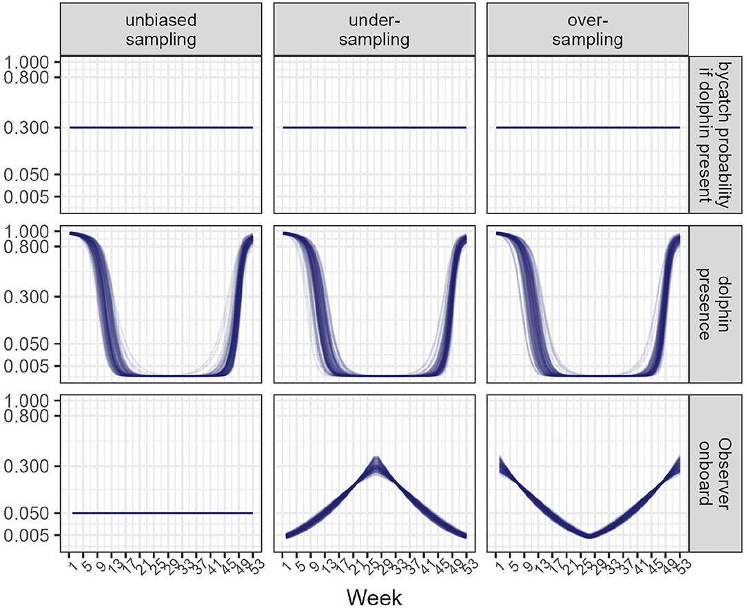
Figure 1. Inputs for data simulation. Top: bycatch probability if dolphins are present during a fishing operation. Middle: dolphin presence during a year. Bottom: Probability for a skipper to accept an observer onboard. Left: sampling is unbiased; Middle column: sampling is biased downwards (under-sampling). Right: sampling is biased upwards (over-sampling). Each line corresponds to one of the 100 data simulations that were carried out. The y-axis is on a square-root scale to better visualize small values.

Bycatch events were simulated for each fishing operations during a day when an observer was present from a Bernoulli distribution according to the product of bycatch probability given dolphin presence and dolphin presence probability for that day. If no observer was present, no data were recorded. The data-generating mechanism used a parametric function for dolphin presence probability and was different from the statistical model used to analyzed the data (see https://gitlab.univ-lr.fr/mauthier/regularized_bycatch). For each sampling scenario, 100 datasets were generated for 1, 5, 10, or 15 years. All data simulations were carried out in R v.4.0.1 (R Core Team, 2020). When simulating only 1 year of data, Equation (2) is not necessary as there is no between-year variation to estimate: the model can be simplified with the omission of β_l. Our Monte Carlo study had a comprehensive factorial design crossing (a) sampling regime (either unbiased or not) and (b) sample size as controlled with the number of years for which the observer programme was assumed to have been in operation.

2.3. Estimation

Estimation of the parameters of model 1 from simulated data was carried out in a Bayesian framework using programming language Stan (Carpenter et al., 2017) called from R v.4.0.1 (R Core Team, 2020) with library Rstan (Stan Development Team, 2020). Stan uses Hamiltonian dynamics in Markov chain Monte Carlo (MCMC) to sample values from the joint posterior distribution (Carpenter et al., 2017). Weakly-informative priors

$\begin{array}{l}\text{were used for regularization:\hspace{0.17em}}\{\begin{array}{l}\mu ~N(0,\frac{3}{2})\hfill \\ \text{prop}~D(1,1,1)\hfill \\ {\sigma }_{\text{total}}~GG(\frac{1}{2},\frac{1}{2},\frac{\log 2}{10})\hfill \end{array}\end{array}$

where ${D}()$ denotes the Dirichlet distribution for modeling proportions (such that $\sum _{i=1}^3\text{pro}{\text{p}}_i=1$) and ${GG}()$ the Gamma-Gamma distribution for scale parameters (Griffin and Brown, 2017; Pérez et al., 2017). With this simplex parametrization, chosen to improve mixing and ease estimation with Monte Carlo methods (He et al., 2007), the several variance components of

$\begin{array}{l}\text{the model were:\hspace{0.17em}}\{\begin{array}{l}{\sigma }_{\text{vessel}}^2={\sigma }_{\text{total}}^2\times {\text{prop}}_1\hfill \\ {\sigma }_{\text{week}}^2={\sigma }_{\text{total}}^2\times {\text{prop}}_2\hfill \\ {\sigma }_{\text{year}}^2={\sigma }_{\text{total}}^2\times {\text{prop}}_3\hfill \end{array}\end{array}$

These priors are weakly-informative (Gabry et al., 2019): the prior for the intercept covers the whole interval between 0 and 1 on the probability scale but is informative on the logit scale. The prior for the scale (square-root of the variance) is heavy tailed and has a median set to $\frac{log10}{2}$ (Griffin and Brown, 2017; Pérez et al., 2017), which translate an assumption about the plausible range of variations in bycatch risk spanning a priori two full order of magnitude from one tenth to a ten-fold increase compared to the mean bycatch rate. Thirty random realizations from our choice of priors are depicted on Figure 2: the whole interval between 0 and 1 is covered, and between-week variations can be large or small.

FIGURE 2

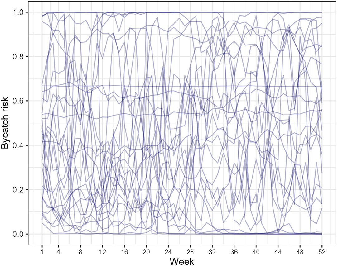
Figure 2. Prior predictive checks sensu (Gabry et al., 2019). Bycatch risk (p_ijkl in Equation 1) is depicted: 30 random realizations from the priors are depicted.

For each simulated dataset, four chains were initialized from diffuse random starting points (Carpenter et al., 2017, p. 20) and run for a total of 1,000 iterations, discarding the first 500 as warm-up. Default settings for the No-U-Turn Sampler (NUTS) were changed to 0.99 for adapt delta and 15 for max treedepth (Hoffman and Gelman, 2014). NUTS uses Hamiltonian Dynamics in MCMC and typically requires shorter runs than other MCMC algorithms both to reach convergence and to obtain an equivalent Effective Sample Size from the posterior (Hoffman and Gelman, 2014; Monnahan et al., 2017). Parameter convergence was assessed using the $\widehat{R}$ statistics (Vehtari et al., 2019) and assumed if $\widehat{R}<1.025$. Upon diagnosing convergence of all parameters, a combined sample of 4 ×500 = 2, 000 MCMC values were obtained to approximate the joint posterior distribution. Let ${\widehat{\mu }}^{\left[m\right]},{\widehat{\beta }}_{kl}^{\left[m\right]},{\widehat{\sigma }}_{\text{vessel}}^{\left[m\right]}$ denote the mth MCMC sample for parameters μ, β_kl and σ_vessel. Bycatch risk ${\widehat{\text{p}}}_{j^{*}kl}$ for a randomly chosen vessel j^* operating in week k of year l was computed from the mth MCMC draw from the joint posterior distribution as:

$\begin{array}{ll}{\widehat{\text{p}}}_{j^{*}kl}^{\left[m\right]}=\text{logi}{\text{t}}^{-1}\left({\widehat{\mu }}^{\left[m\right]}+{\widehat{\beta }}_{kl}^{\left[m\right]}+{\widehat{\alpha }}_{j^{*}}^{\left[m\right]}\right)& (4)\end{array}$

where ${\widehat{\alpha }}_{j^{*}}^{\left[m\right]}~{N}(0,{\widehat{\sigma }}_{\text{vessel}}^{\left[m\right]})$. This predicted bycatch risk incorporates between-vessel variability, that is it takes into account the fishing style of skippers. The predicted risk (on a logit scale) for a random chosen skipper is ${\widehat{\alpha }}_{j^{*}}^{\left[m\right]}$ and was drawn from the posterior predictive distribution: not all skippers may be observed in the sample, and but the subset of skippers that accept an observer can be used to estimate a between-skipper variance in bycatch risk. In practice, the number of fishing operations carried out in the course of a week in a year by individual skippers is unknown, although the aggregated number of fishing operations may be known. If totals by skippers were available, and all skippers had been sampled, it would be more efficient to use skipper-specific estimated risk, but we did not assume that this would necessarily be the case.

The total number of bycatch events, T_bycatch was estimated as the average over the 2,000 MCMC draws from the posterior:

$\begin{array}{ll}{\widehat{T}}_{\text{model}-\text{based bycatch}}=\frac{1}{2000}{\displaystyle \sum _{m=1}^{2000}}\left({\displaystyle \sum _{l=1}^{n_{\text{year}}}}{\displaystyle \sum _{k=1}^{n_{\text{week}}}}{\widehat{\text{p}}}_{j^{*}kl}^{\left[m\right]}\times N_{kl}\right)& (5)\end{array}$

where N_kl is the total number of fishing operations that took place is week k of year l. The total number of strata for post-stratification was n_year×n_week, with a maximum of 15 ×52 = 780 cells. Highest Posterior Density credible intervals at the 80% level were computed with function HPDinterval from package coda (Plummer et al., 2006) for uncertainty evaluation. Equation (5) is an instance of a ratio-estimator with post-stratification, except that it uses model-based estimates of bycatch risk. This model-based approach regularizes estimates with partial pooling (Gelman and Shalizi, 2013): the variance of estimates is greatly reduced by introducing some bias with structured priors (Gao et al., 2019). Our results were benchmarked against an approach similar to that of ICES WGBYC whereby total number of bycatch events was estimated1 as:

$\begin{array}{ll}{\widehat{T}}_{\text{design}-\text{based bycatch}}={\displaystyle \sum _{l=1}^{n_{\text{year}}}}\left({\bar{p}}_l\times {\displaystyle \sum _{k=1}^{n_{\text{week}}}}{N}_{kl}\right)& (6)\end{array}$

where ${\bar{p}}_l$ is the average bycatch risk estimated as the mean from the observed sample in year l. Confidence intervals at the 95% level were computed using either the bootstrap or the Clopper-Pearson approach as customary in ICES WGBYC. Both were considered as the Clopper-Pearson approach is known for being more conservative: it produces confidence intervals that above the nominal level (i.e., wider than necessary) but generates non-nil confidence intervals even if no bycatch has been observed (Northridge et al., 2019). In practice, ICES WGBYC often pooled several years to stabilize the estimate of $\bar{p}$ (e.g., ICES 2018, p. 57–58; Carretta and Moore, 2014): Equation (6) translate an ideal case that is rarely met in practice. ICES WGBYC usually works on bycatch rates (in number of PETS per unit effort), not bycatch risk. We focused on risk for simplicity, but scaling bycatch risk to a rate is straightforward by multiplying with the average number of PETS bycaught in a bycatch event. Dolphin presence was seasonal in the data-generating mechanism for simulations: pitching a method that can explicitly accommodate such seasonality against one that does not may be viewed as knocking down a strawman. However, current estimates of PETS bycatch in Europe are stratified by flag, ICES statistical areas, and métiers but not by season (e.g., Table 2 p. 17 in ICES 2019; Northridge et al., 2019, p. 27). The comparison remains relevant and topical as it matches current practices.

3. Results

Convergence across all simulations and scenarios was assumed to be reached, with all $\widehat{R}<1.025$, for all parameters. For each simulation, chains were combined in a single sample of 2,000 values to approximate the joint posterior distribution of the model defined by Equations (1), (2), and (3).

3.1. Design- vs. Model-Based Approach

Comparing the design- and model-based approach was done with simulating 1 year of data. When data sampling was unbiased, both the design- and model-based approach were able to recover the true number of bycatch events (Figure 3; Table 1). Estimates of bycatch events were statistically unbiased but their precision low with a (frequentist 95%) confidence or (Bayesian 80%) credible interval (CI) as large as 100% of the point estimate (Table 1), as could be expected with only 15 bycatch events were recorded on average by onboard observers (Table 1). With under-sampling, design-based estimates were negatively biased (that is, they were under-estimates) whereas model-based estimates were still unbiased on average (Figure 3; Table 1). With over-sampling, design-based estimates were positively biased (that is, they were over-estimates) but so were model-based estimates, although bias was 5 times smaller (Figure 3; Table 1). In all cases, coverage was 100% but largely as a result of low precision: precision was very low with CI spanning some 200% of the point estimate for the unbiased and under-sampling scenarios. This low precision was the result of having to work with as few as 5 observed bycatch events on average (Table 1). Precision improved with over-sampling, but was still as high as 50% of the point (over-)estimate. The model-based approach was well-calibrated in both the unbiased and under-sampling scenarios (Figure 4): model-based estimates were on average equal to the truth whereas this was only the case with design-based estimates when sampling was unbiased. In addition, the model-based approach was able to recover the temporal profile of bycatch risk (Figure 5) in these two scenarios, but with an increased accuracy and precision if sampling was unbiased. In the over-sampling scenario, both the design- and model-based approaches were not well -calibrated (Figure 4) and the model-based approach over-estimated bycatch risk when no data were collected (Figures 1, 5).

FIGURE 3

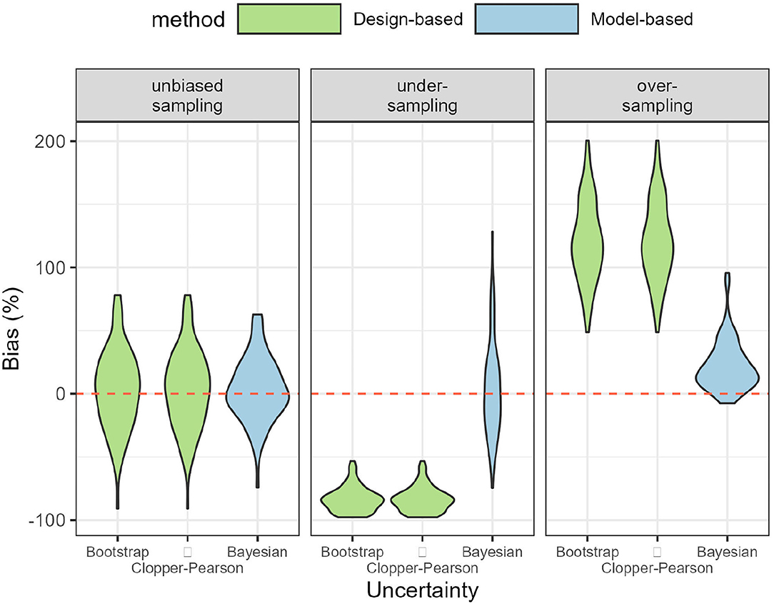
Figure 3. Violin plot of bias in point estimates of total bycatch events. Left: data sampling was unbiased and all methods yielded statistically unbiased estimates. Middle: Under-sampling scenario: only the model-based approach was accurate. Right: Over-sampling scenario: both the design- and model-based approaches were biased upwards. Violin plots are based on 100 simulations.

TABLE 1

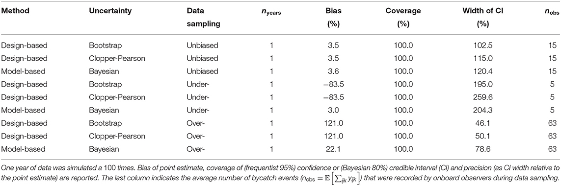
Table 1. Statistical properties of estimates from the design- and model-based approach.

FIGURE 4

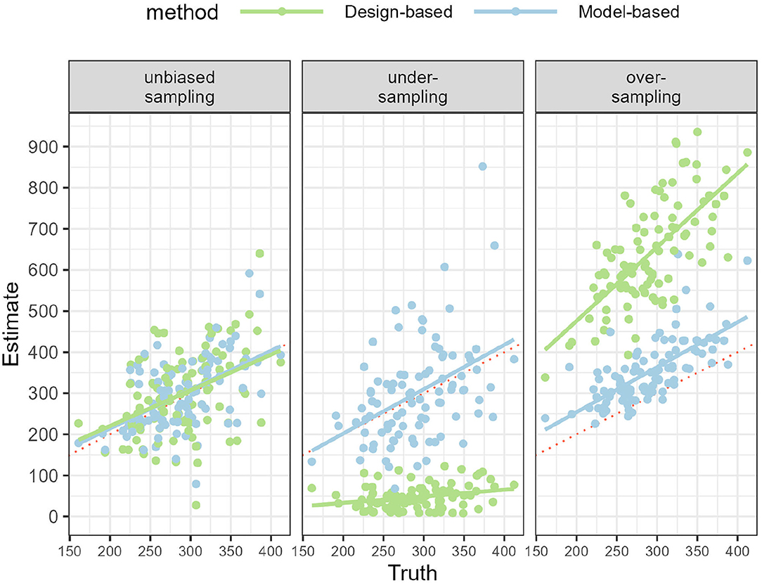
Figure 4. Regression lines of point estimates against the true number of bycatch events, showing the calibration of the design- and model-based approach. The x-axis shows the true number of bycatch events across 100 simulations, spanning between 150 and 400 events. The red dotted line shows the identity line, i.e., no bias. Left: data sampling was unbiased and all methods yielded statistically unbiased estimates. Middle: Under-sampling scenario: only the model-based approach was well-calibrated. Right: Over-sampling scenario: both the design- and model-based approaches were not calibrated to the truth.

FIGURE 5

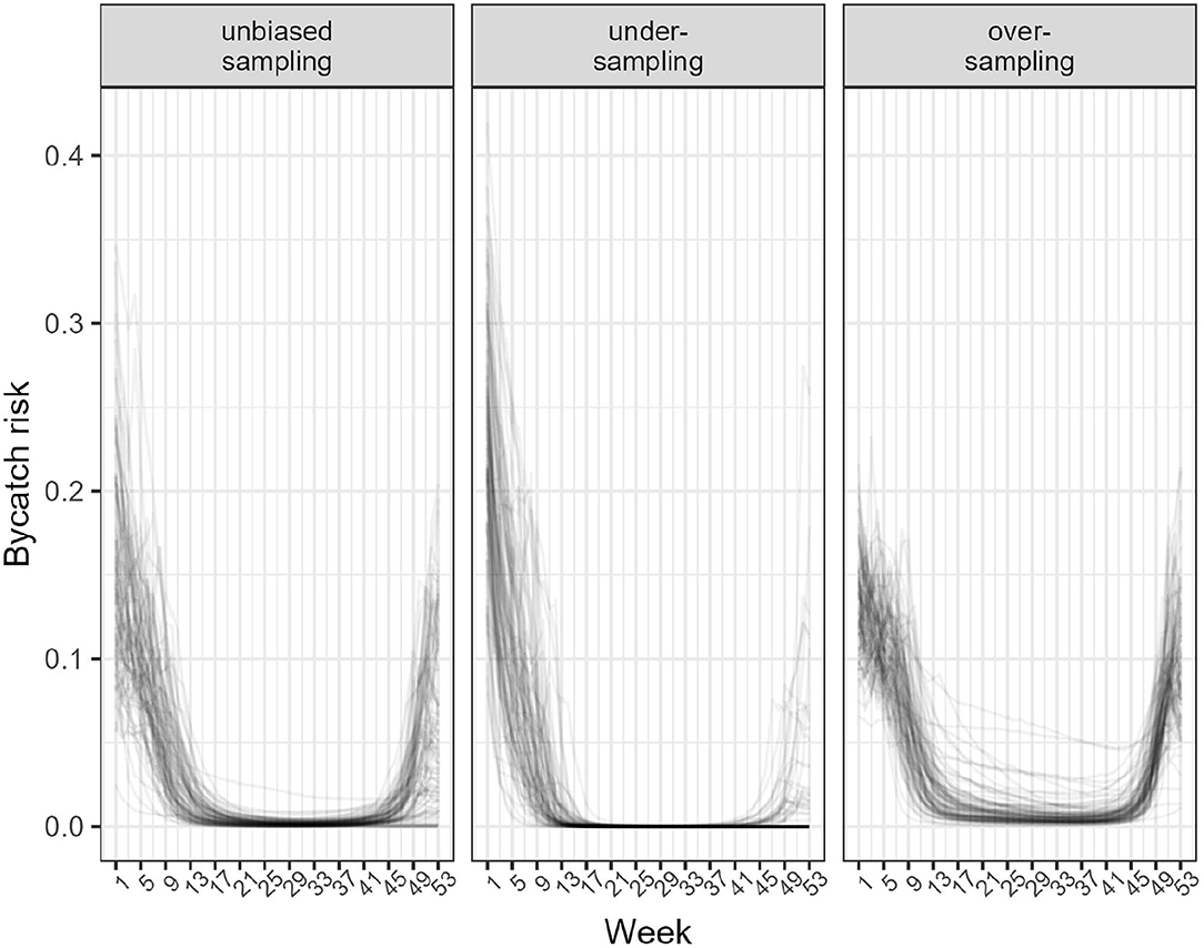
Figure 5. Estimated temporal pattern in mean bycatch risk from the model-based approach. Left: data sampling was unbiased. Middle: Under-sampling. Right: Over-sampling. The model-based approach recovered the correct pattern overall, but overestimated risk in the over-sampling scenarios when risk was, in fact, nil but no data were collected.

3.2. Model-Based Approach With Several Years of Data

With several years of data, the model-based approach was able to yield nearly unbiased estimates: the bias was smaller than 3 bycatch events when sampling was unbiased, but as large as 10 (on average) with biased sampling and 3 years of data. The precision of estimates improved with several years of data, as expected with larger sample size. Precision of model-based estimates with over-sampling were already acceptable with 3 years of data: an 80% credible interval width of 50% corresponds to a coefficient of variation of $\frac{50}{2.5}\approx 20$% assuming a normal distribution for the posterior. The model-based approach allowed to obtain estimates at the weekly scale (Figure 6): these estimates were approximately unbiased in the unbiased and over-sampling scenarios, but were biased for the under-sampling scenario. In that latter case, the bias was correlated with the temporal pattern used to simulate dolphin presence (Figure 1): it was the largest when dolphin presence was at its highest but positive at the beginning of a year and negative at the end of the same year. Both biases were greatly attenuated with increased sample size.

FIGURE 6

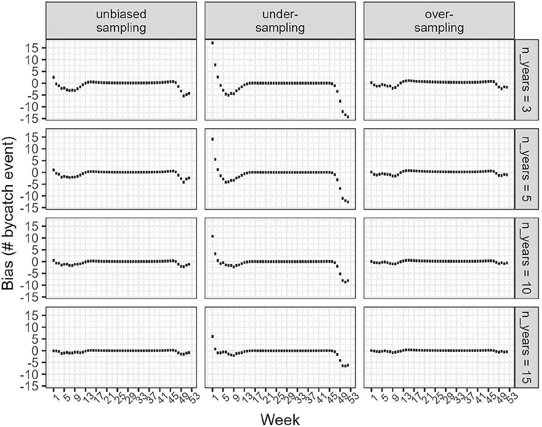
Figure 6. Box plots of bias (in number of estimated bycatch events compared to the truth) in the weekly model-based estimates of bycatch events. Left: data sampling was unbiased. Middle: Under-sampling. Right: Over-sampling. Each row corresponds to data simulated for a different number of years.

4. Discussion

Using Monte-Carlo simulations, we investigated the statistical properties of a model-based approach, regularized multilevel regression with post-stratification, to estimate the total number of bycatch events in a fishery operating year-round. Simulations were broadly informed from the case of common dolphins and pair-trawlers in the Bay of Biscay and from harbor porpoises and set-gillnets in Celtic Seas. A salient feature of simulations was biased sampling with observers being preferentially accepted onboard when bycatch risk was either high or low. Data simulations in that latter case, which is the most realistic one in the Bay of Biscay (Peltier et al., 2016), resulted in as few as 5 observed bycatch events per year on average (Tables 1, 2). This aligns with the ubiquitous description of small cetacean bycatch being a rarely observed event. It was nevertheless possible to fit a regularized multilevel regression model on these data. Importantly, estimates from this model-based approach were statistically less biased than the design-based estimates when sampling was biased. Model-based estimates were, however, imprecise but this is largely to be expected (Amandè et al., 2012), especially with as few as 5 observed bycatch events per year. The design-based approach was also imprecise, even in the unbiased data sampling scenario of 5% coverage of the fleet, which is not reached in practice (Anonymous, 2016; ICES, 2020b). The design-based approach was very sensitive to how data were collected: this approach severely under- or over-estimated bycatch when sampling was biased, whereas the model-based approach was still well-calibrated with under-sampling, but not with over-sampling (Figure 4).

TABLE 2

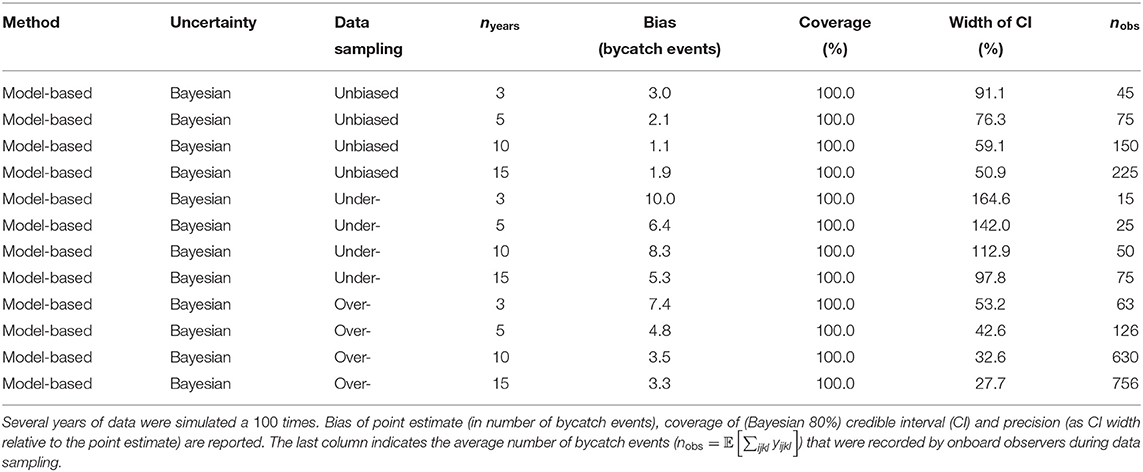
Table 2. Statistical properties of estimates from the model-based approach.

Biases in onboard observer data are pervasive and widely acknowledged (Babcock and Pikitch, 2003; Benoît and Allard, 2009; Peltier et al., 2016). Enforcing coverage as required to achieve a pre-specified precision in estimates can be challenging in practice. For example, in 2016, France only achieved a coverage rate less than 2% for most métiers and concluded on the impossibility of scaling-up observed bycatch rates to the whole fleet (Anonymous, 2016, p. 24). There were, however, 9 bycatch events of common dolphins in pair-trawlers targeting European hake (Merluccius merluccius). From these numbers, bycatch was described a “rare” event (Anonymous 2016, p. 23). Such a conclusion would be warranted if sampling were representative, in which case the design-based estimate could be used, even though its precision would still be very low. On the other hand, with under-sampling, this conclusion is misleading as our simulations further illustrated: although only 5 bycatch events were observed on average (Figure 4), the true number of bycatch events was on average 60 times larger (Figure 4). In our simulations, the true bycatch rate was on average ≈3% over a year, which is not rare, but not frequent either. Moreover, interviews with French skippers deploying trawls or gillnets in the Bay of Biscay revealed that more than 80% of respondents declared to having experienced at least one small cetacean bycatch event in a year (Cloâtre, 2020). Such a large proportion contradicts the idea of common dolphin bycatch being a rare event in the Bay of Biscay, but rather suggest severe biases in onboard observer data that result in the rare reporting of bycatch events, rather than a rarity of events per se. The common dolphin in the Bay of Biscay illustrates how under-sampling may distort the perception of bycatch as a very rare event when it can, in fact, be widespread. This is a catch-22 situation whereby cetacean bycatch is described as a rare event because it is rarely reported, and this perceived rarity may serve to argue against ambitious dedicated monitoring programmes out of cost-effective considerations, thereby preventing to dispel the initial misconception.

Finding an optimal sampling plan for fisheries with rare bycatch events is a long standing problem (ICES, 2009). Several strategies have been attempted: for example in the United States, one strategy is “pulsed sampling” whereby a particular fishery or métier is very heavily sampled for a short period of time in order to maximize the chance for observers to record any bycatch that might occur (ICES, 2009). This pulsed sampling strategy corresponds to our over-sampling scenario wherein monitoring effort is positively correlated with bycatch risk. Under this scenario, the absence of any sampling at all when bycatch risk was low was detrimental to the accurate estimation of bycatch events with our model. Model-based estimates were, however, less biased than design-based estimates. Arguably, this comparison is somewhat artificial as a correct comparison would use all the available information and uses estimators that are season-specific to account for under-sampling when bycatch risk is low if such a period is known to the investigator. Notwithstanding this shortcoming, model-based estimates represented an improvement and allowed to infer the bycatch risk profile accurately, especially with several years of data.

We showed with our Monte-Carlo simulations that regularized multilevel regression with post-stratification can nevertheless be used to analyze bycatch data despite concerns about non-representative sampling. Model-based approaches (Palka and Rossman, 2001), with post-stratification (Lennert et al., 1994), or machine learning (Carretta et al., 2017), or multilevel regression (Sims et al., 2008; Martin et al., 2015) have previously been used to estimate bycatch rates. Traditional, design-based, ratio estimates are biased if sampling is biased; imprecise if observer coverage is low (as is the usual case in the North East Atlantic; see for example Figure 14, p. 114 in ICES, 2020b); and volatile if bycatch events are only observed occasionally (Carretta et al., 2017). The traditional remedy to stabilize estimates and improve precision is to bypass year-specific estimation and pool several years together (Carretta and Moore, 2014; ICES, 2018). This pragmatic solution improves precision but does not address the problem of biased sampling. It also introduces estimation bias for any year-specific estimates by pooling completely several years in order to stabilize the variance of estimates (ICES, 2009, p. 36): any between-year differences are thus ignored in order to obtain a better precision of estimates. It is a reasonable approach in practice, but one that can be improved. Model-based approaches offer a trade-off between no-pooling (keeping all years separate) and complete-pooling with a third option: partial pooling or regularization (Gelman and Shalizi, 2013). Regularization is a general term for statistical procedures that give more stable estimates. Our model-based approach achieves regularization by leveraging, via a structured prior model (Equations 2 and 3, see section 2), the within-year information at the weekly scale. The result were more stable and accurate annual bycatch estimates at the cost of some modeling assumptions and weakly-informative priors. Importantly, weekly estimates could also be obtained with our model-based approach.

Our model-based approach is semi-parametric as it uses a random walk prior to learn from the data the weekly pattern in bycatch risk. This prior is also ensuring some smoothness in the temporal risk profile as it translates an assumption on the correlation between 2 consecutive weeks. This random walk model remains simple as the order is fixed to 1. We further expanded this model to allow for between-years variation in the weekly risk profile with a Gaussian Process prior (Neal, 1998; Goldin and Purse, 2016). Importantly, these two prior choices (a random walk and a Gaussian Process prior) add structure to the model and help in leveraging the information present in the sparse data typical of onboard observer programmes. Even when with over-sampling, these choices were not detrimental as model-based estimates were statistically unbiased and precise with 3 years of data (Table 2). The explicit consideration of time effects is key to mitigate bias in sampling. In our simulations, dolphin presence was caricaturally seasonal, and observers could be preferentially allowed on fishing vessels when dolphins were less or more likely to be present (Figure 1). Our model was still able to provide statistically unbiased estimates of bycatch in those scenarios, although these estimates were very imprecise with under-sampling. However, they were not more imprecise than the traditional (but biased) design-based estimates (Table 1) if 80% credible interval were used. In addition to being unbiased, these estimates could also reveal with accuracy the temporal risk profile (Figure 5). It is important to keep in mind here that our model is different from the data-generating model used in simulating data: our results were not simply an instance of using a true model, which is impossible in practice as a model is by definition a simplification used to capture the salient features of a phenomenon. Our model had some shortcomings: for example, bias increased with 3 years of data compared to 1 year for the under-sampling scenario (contrast Tables 1, 2). This increased bias (toward the prior model) was the result of partial pooling but came with a gain in precision as evidenced in the width of credible intervals. The bias progressively wore off with more years of data, illustrating thereby the attractiveness of partial pooling and structured priors to regularize estimates (Gelman and Shalizi, 2013; Gao et al., 2019). The gain in reducing bias in estimates and increasing their precision was most evident with over-sampling (Tables 1, 2).

Our model could also provide weekly bycatch estimates which were largely unbiased except in the under-sampling scenario where a positive and negative bias remained at the beginning and end of a year respectively, even with 15 years of data (Figure 6). With under-sampling, few observed bycatch events can be collected by design because observers are very unlikely to be accepted on board by skippers. Weekly estimates were too high at the beginning of a year but too low at the end, but this somewhat canceled out at the year-level. There was still a slight overestimation bias resulting from our choice of a non-symmetric pattern for dolphin presence and a symmetric pattern for biased coverage: observing bycatch events at the end of a year was comparatively more difficult than at the beginning of a year because overlap between a non-nil coverage and dolphin presence was smaller at the end of year (Figure 1). These shortcomings illustrate that a model-based approach should be tailored to the context of the study, and we designed our simulations largely from our knowledge on the common dolphin in the Bay of Biscay. However, the framework of regularized multilevel regression with post-stratification is very flexible and we believe our proposed model has large potential for generality as it simply translates a decomposition of bycatch risk into a smooth time-varying and (unstructured) time-invariant effects. The model can easily be made more complex, data permitting, to accommodate spatial effects with, for example, a Besag-type prior (Sims et al., 2008; Morris et al., 2019).

Several important assumptions are structurally built into our model: in particular, a first order random was assumed for the mean function of the Gaussian Process prior, with no attempt to estimate from data the correlation parameter (e.g., using an AR(1) prior instead). The choice of a first order random walk was not aiming at uncovering the true data-mechanism: our aim were to reveal a temporal pattern in bycatch risk from sparse data using a flexible, yet parsimonious approach. This was particularly true in the under-sampling scenario where few bycatch events could be observed in any given year of simulated data. In the other scenarios, other choices than the first order random walk could be considered as more data are collected. We also assumed that the range parameter of the covariance function in the Gaussian Process prior for week effects was known and such that bycatch risk was temporally uncorrelated after 4 weeks. Fixing the range parameter is usually not recommended but was motivated by consideration of the data-to-parameter ratio, and computation convenience. Bycatch data are binary and can be sparse: these two features underscore how little information may be available. In this context, limiting the number of parameters to estimate can be justified on pragmatic consideration. The model we are proposing is parameter-rich, but some structure are assumed on these parameters in the form of the prior used. These priors represent choices from the analyst and may be reconsidered and tested, data permitting. There was some evidence that bycatch risk was under-smoothed in the over-sampling scenario which resulted in an over-estimation of bycatch risk (Figure 5, rightmost panel). Model expansion is seamless with Stan (Gabry et al., 2019), and the above mentioned parameters could be estimated, rather than fixed, with adequate data. Despite somewhat arbitrary prior and modeling choices, our model provided more accurate estimates of bycatch numbers and bycatch risk in under- and over-sampling scenarios. This satisfactory predictive ability points to another important limitation.

Our model is phenomenological, i.e., it is agnostic of the causes behind the temporal variations in bycatch risk. Bycatch risk is the product of dolphin presence and bycatch probability given presence (the latter was constant in our simulations). The model only estimates this product of two probabilities and thus cannot disentangle them without other sources of data. This limitation seems inconsequential in our simulations for the aim of accurate estimation of the total number of bycatch events as interest lies in the effects of causes (how much bycatch?) rather than in the causes of effects (why bycatch occurred?). A straightforward model expansion (as pointed out by a reviewer) would be the consideration of p vessel-level covariates (z_1j, …, z_pj) in Equation (1):

$\begin{array}{ll}{\alpha }_j~{N}\left({\displaystyle \sum _{b=1}^p}({\xi }_b\times z_{jb}),{\sigma }_{\text{vessel}}\right)& (7)\end{array}$

Candidate covariates such as vessel length or gear-attributes (e.g., mesh size) could be incorporated in the analysis to improve the exchangeability assumption on vessel-effects. An obvious covariate to consider for detecting self-selection of skippers into observer programme participation is to include whether a skipper has ever accepted an observer, or the number of times it did so in the past: a negative regression coefficient could be interpreted as voluntary skippers having an intrinsically lower risk of bycatch. Including skipper-level covariates could reduce the between-skipper variance ${\sigma }_{\text{vessel}}^2$, and improve ultimately precision of bycatch estimates. Consideration of other distributions than the normal (e.g., a skew-normal, or a Student-t distribution with a fixed degree of freedom) would be straightforward with Stan but is probably worthwhile only with large enough amount of data for all practical purposes (McCulloch and Neuhaus, 2011).

An important assumption underlying accurate estimation is that the information on the total effort must also be accurate and available at the scale of weeks for post-stratification. This assumption is crucial to scale-up estimates from the (potentially biased) sample to the population, but it does not necessarily hold with fisheries effort as the latter is more often estimated rather than measured directly (Julian and Beeson, 1998; ICES, 2018, 2020b). Here we assumed that the total number of fishing operations (e.g., number of tows for trawls; Tremblay-Boyer and Berkenbusch, 2020) are available as auxiliary information for post-stratification. This assumption about the availability of disaggregated data stems from the explicit consideration of time as an important predictor of variations in bycatch risk. This assumption is necessary for using post-stratification to align the sample with the population targets but may be difficult to meet in practice. Currently, ICES WGBYC uses in its BRA a coarse, but admittedly comparable proxy across fisheries and countries to quantify fishing effort, namely days at sea (ICES, 2019). A day at sea is any continuous period of 24 h (or part thereof) during which a vessel is present within an area and absent from port (Anonymous, 2019a). Importantly, this definition is not at the level of a fishing operation, and effort thus quantified is already aggregated at a level above that at which bycatch data are collected. This coarsening of fisheries effort data is fundamentally a measurement problem, and one that modeling should not be expected to remedy easily. BRA uses an estimate of total fishing effort for the fisheries of concern in a specific region, together with some estimate of likely or possible bycatch rates that might apply for the species of concern, in order to evaluate whether or not the total bycatch in that area might be a conservation issue. A regularized multilevel regression model could be used to obtain estimates of bycatch rates to be used in BRA. Post-stratification could also be attempted using the coarse days at sea proxy for effort, and thus our framework could be adapted to match the requirements of ICES WGBYC.

Assuming that our framework were to be adopted to produce bycatch estimates, how would both fisheries and Non-Governmental Organizations (NGOs) react given the salience of bycatch as a policy issue in Europe? Such a prospective question inevitably entails some speculations (as with all “what-if” questions), but may nevertheless bring some insights as highlighted by a reviewer. Within Europe, the conservation reference currently available for assessing bycatch is that established under the Agreement on the Conservation of Small Cetaceans of the Baltic, North East Atlantic, Irish and North Seas. The agreement has the conservation objective to minimize anthropogenic removals of harbor porpoises (and other small-sized cetaceans), and to restore and/or maintain population depletion to/at 80% or more of the carrying capacity in each assessment unit (ASCOBANS, 2000; ICES, 2020c). Methods for setting conservation reference points were agreed in March 2021 at the meeting of the Biodiversity Committee of the Olso-Paris Regional Sea Convention. This committee adopted the use of the Removals Limit Algorithm for harbor porpoises in the North Sea assessment unit and a modified Potential Biological Removal (Wade, 1998) for common dolphins in the North-East Atlantic (Genu et al.)³. Accurate bycatch estimates will be needed for assessment against these reference points. However, fisheries may challenge the accuracy of estimates precisely because they will result from a new statistical model. While a healthy skepticism is warranted, and model improvements are certainly possible, it must be kept in mind that our model only addresses the issue of having a correlation between observer coverage and bycatch risk, and does so with some assumptions. There would remain many biases to be addressed in bycatch data (Babcock and Pikitch, 2003), and many of them would be best addressed with a proper random allocation of professional observers to vessels (that is better design and better measurement). A purely model-based solution can be brittle (Sarewitz, 1999), and may lead to displacement of the problem of bycatch assessment to a never-ending problem of model improvement that would delay any corrective measures or decision (Rayner, 2012). Model-based estimates offer a pragmatic approach to the analysis of already collected data, but should not deflect from improving survey design where possible. Assuming that model-based estimates would be endorsed by a fishery industry, NGOs could challenge in court any reference point that is not zero for PETS, since by definition, it ought to be zero. The Habitats Directive requires strict protection and prohibits “all forms of deliberate capture or killing” (emphasis added) of all species listed on its Annex IV which includes all cetacean species. The Court of Justice of the European Union has consistently ruled that the adjective “deliberate” is to be understood in the sense of “conscious acceptance of consequences” (Trouwborst and Somsen, 2019): in other words, using knowingly a gear that may potentially catch a protected species contravenes the Habitat Directives. What will eventually play out remains to be seen, but strongly hinges on how polarized the bycatch issue is. As scientists, our duty remains to provide the best available evidence on bycatch and to outline all management actions and their consequences in light of this evidence (Pielke, 2007). Our model is unlikely to change bycatch management in France in the near term: both fisheries and NGOs are at loggerheads, vying for public and official support. They are building constituencies and advertising unyielding positions in diverse medias: we content that a legal confrontation at a national or supra-national level is extremely likely and probably being prepared. We nevertheless think our model, by making use of data already collected within the DCF framework and by encouraging further, ideally dedicated, monitoring; can be part of a messy solution to the wicked problem (Frame, 2008) of dolphin bycatch in the medium to long term, once the gavel hits and the dust settles.

5. Conclusion

We investigated with simulations the ability of multilevel regularized regression with post-stratification to estimate cetacean bycatch for observer programmes when coverage is correlated to bycatch risk. Our aims were to provide a first investigation on model-based estimates obtained from samples preferentially collected either during low- or high-bycatch risk periods. The unbiased sampling case is unrealistic (Babcock and Pikitch, 2003): biased sampling, either under-sampling or over-sampling (ICES, 2009), may be the general case. We considered both of these cases, under quite extreme scenarios whereby data collection was highly correlated with bycatch risk, resulting in either very few observed events with under-sampling, and a large number of observed events with over-sampling. In both cases, multilevel regularized regression with post-stratification was able to produce nearly unbiased bycatch estimates with as few as 5 observed events data. With only 1 year of data, precision was low, especially with under-sampling, and there was some estimation bias with over-sampling one. These results stemmed from the extreme scenarios we considered but illustrate nevertheless that a model cannot be expected to solve all the deficiencies of data collection and measurement. Good measurement is key for accurate estimation and our results actually re-emphasize the importance of design. However, they also show that a good data collection design and an adequate modeling framework are synergistic and allow to extract a lot of information for sparse data. Assuming a normal distribution for the bycatch estimates (which is not necessary as the posterior is available, but the following are back-of-the-envelope calculations to be used for deriving heuristics), a 80% Bayesian CI width divided by 2.5 gives an idea of the associated coefficient of variation: the model-based approach can yield a coefficient of variation of 50% with as few as 15 observed events if sampling is unbiased. With under-sampling, one would need 10 years of data (under our data simulation schemes) to obtain the same precision. This re-iterates the need to (i) have dedicated observer schemes, (ii) ensure adequate observer coverage and (iii) use a model-based approach tailored to extract as much information as possible from sparse data, as the first two points are very difficult to live up to in practice.

The key assumptions behind regularized multilevel regression with post-stratification in our simulations are that bycatch risk changes smoothly through time and that accurate data on the number of fishing operations at the same temporal scale are available (e.g., number of tows for trawls; Tremblay-Boyer and Berkenbusch, 2020). When both assumptions can be reasonably entertained, we showed how a model-based approach using recent methodological developments is attractive, irrespective of how data were collected. A further asset of the explicit consideration of a temporal scale is that it may help in pinpointing more precisely windows of heightened risk in order to target adequate mitigation measures (e.g., spatio-temporal closures). The framework of multilevel modeling is very flexible and can accommodate spatial effects, etc., data permitting. Regularization will, in general, be needed to mitigate data sparsity and leverage partial pooling in order to obtain stable estimates of bycatch. Given the satisfactory performance of regularized multilevel regression with post-stratification in our simulations, we recommend further investigations using this technique to estimate bycatch rate and numbers from both representative or non-representative samples. The modeling choices we made (e.g., a first order random walk for the mean function, or fixing the range parameter in the covariance function of the Gaussian Process prior) are not prescriptive, and other choices of prior models for parameters should be investigated. Investigations should be tailored to the context, and modeling choices motivated by the latter: given the complexity of PETS bycatch, a one-size-fits-all solution is unlikely. A re-analysis of >15 years of observer data on common dolphin bycatch in pair trawlers flying the French flag is currently underway (Rouby et al.)⁴ in order to obtain better bycatch estimates that could be further used to estimate conservation reference points in order to better manage this fishery in the long run (Cooke, 1999; Punt et al., 2021).

Data Availability Statement

The datasets presented in this study can be found in online repositories. The names of the repository/repositories and accession number(s) can be found below: https://gitlab.univ-lr.fr/mauthier/regularized_bycatch.

Author Contributions

MA: led the analyses, the conception, and writing of the paper. ER and KM: support in analyses, paper conception, and writing. All authors contributed to the article and approved the submitted version.

Funding

ADERA and JNCC provided support in the form of salaries for MA and KM, respectively, but did not have any additional role in the study design, data collection and analysis, decision to publish, or preparation of the manuscript.

Conflict of Interest

MA is employed by the commercial company ADERA which did not play any role in this study beyond that of employer.

The remaining authors declare that the research was conducted in the absence of any commercial or financial relationships that could be construed as a potential conflict of interest.

Publisher's Note

All claims expressed in this article are solely those of the authors and do not necessarily represent those of their affiliated organizations, or those of the publisher, the editors and the reviewers. Any product that may be evaluated in this article, or claim that may be made by its manufacturer, is not guaranteed or endorsed by the publisher.

Acknowledgments

We thank two reviewers from critical and constructive comments that help in improving the present manuscript. MA thanks Amaterasu for support when carrying the simulations.

Footnotes

1. ^https://ec.europa.eu/info/news/july-infringements-package-commission-moves-against-member-states-not-respecting-eu-energy-rules-2019-jul-26_en

2. ^https://appsso.eurostat.ec.europa.eu/nui/show.do?dataset=fish_fleet_alt&lang=en

3. ^Genu, M., Gilles, A., Hammond, P., Macleod, K., Paillé, J., Paradinas, I. A., et al. (in preparation). Evaluating strategies for managing anthropogenic mortality on marine mammals: an R Implementation with the Package RLA.

4. ^Rouby, E., Dubroca, L., Cloâtre, T., Demanèche, S., Genu, M., Macleod, K., et al. (in preparation). Estimating cetacean bycatch from non-representative samples (II): a Case Study on Common Dolphins in the Bay of Biscay.

References

Amandè, M. J., Chassot, E., Chavance, P., Murua, H., de Molina, A. D., and Bez, N. (2012). Precision in bycatch estimates: the case of Tuna Purse-Seine Fisheries in the Indian Ocean. ICES J. Mar. Sci. 69, 1501–1510. doi: 10.1093/icesjms/fss106

CrossRef Full Text | Google Scholar

Anonymous (2016). Rapport Annuel sur la mise en øeuvre du Réglement Européen (CE) 812/2004 Établissant les Mesures Relatives Aux Captures Accidentelles de Cétacés dans les Pêcheries. Rapport annuel réglementaire. Technical report, Direction des pêches maritimes et de l'aquaculture (DPMA).

Google Scholar

Anonymous (2019a). Commission Implementing Decision (EU) 2019/910. Establishing the Multiannual Union Programme for the Collection and Management of Biological, Environmental, Technical and Socioeconomic Data in the Fisheries and Aquaculture Sectors. European Commission.

Google Scholar

Anonymous (2019b). Regulation (EU) 2019/1241 of the European Parliament. The Council of 20 June 2019 on the Conservation of Fisheries Resources and the Protection of Marine Ecosystems Through Technical Measures.

Google Scholar

ASCOBANS (2000). Annex O - report of the IWC-ASCOBANS Working Group on Harbour Porpoises. J. Cetacean Res. Manage. 2, 297–305.

Google Scholar

Authier, M., Aubry, L., and Cam, E. (2017a). Wolf in sheep's clothing: model misspecification undermines tests of the neutral theory for life histories. Ecol. Evol. 7, 3348–3361. doi: 10.1002/ece3.2874

PubMed Abstract | CrossRef Full Text | Google Scholar

Authier, M., Saraux, C., and Péron, C. (2017b). Variable selection and accurate predictions in habitat modelling: a shrinkage approach. Ecography 40, 549–560. doi: 10.1111/ecog.01633

CrossRef Full Text | Google Scholar

Avila, I. C., Kaschner, K., and Dormann, C. F. (2018). Current global risks to marine mammals: taking stock of the threats. Biol. Conserv. 221, 44–58. doi: 10.1016/j.biocon.2018.02.021

CrossRef Full Text | Google Scholar

Babcock, E., and Pikitch, E. K. (2003). How Much Observer Coverage is Enough to Adequately Estimate Bycatch? Technical report, Pew Institute for Ocean Science.

Google Scholar

Benoît, H., and Allard, J. (2009). Can the data from at-sea observer surveys be used to make general inference about catch composition and discards? Can. J. Fish. Aquat. Sci. 66, 2025–2039. doi: 10.1139/F09-116

CrossRef Full Text | Google Scholar

Brownell, R. J., Reeves, R., Read, A., Smith, B., Thomas, P., Ralls, K., et al. (2019). Bycatch in gillnet fisheries threatens critically endangered small cetaceans and other aquatic megafauna. Endangered Species Res. 40, 285–296. doi: 10.3354/esr00994

CrossRef Full Text | Google Scholar

Cam, E. (2012). “Each site has its own survival probability, but information is borrowed across sites to tell us about survival in each site”: random effects models as means of borrowing strength in survival studies of wild vertebrates. Anim. Conserv. 15, 129–132. doi: 10.1111/j.1469-1795.2012.00533.x

CrossRef Full Text | Google Scholar

Carpenter, B., Gelman, A., Hoffman, M. D., Lee, D., Goodrich, B., Betancourt, M., et al. (2017). Stan: a probabilistic programming language. J. Stat. Softw. 76, 1–32. doi: 10.18637/jss.v076.i01

CrossRef Full Text | Google Scholar

Carretta, J. V., and Moore, J. E. (2014). Recommendations for Pooling Annual Bycatch Estimates when Events are Rare. Technical report. NOAA-TMNMFS-SWFSC-528, NOAA. NOAA Technical Memorandum.

Google Scholar

Carretta, J. V., Moore, J. E., and Forney, K. A. (2017). Regression Tree and Ratio Estimates of Marine Mammal, Sea Turtle, and Seabird Bycatch in the California Drift Fishery: 1990-2015. Technical Report NOAA-TM-NMFS-SWFSC-568, NOAA. NOAA Technical Memorandum.

Google Scholar

Cloâtre, T. (2020). Projet LICADO - Limitation des Captures Accidentelles de Dauphins Communs dans le Golfe de Gascogne. Bilan des Enquêtes auprés des Professionnels du Golfe de Gascogne (Paris).

Google Scholar

Cooke, J. G. (1999). Improvement of fishery-management advice through simulation testing of harvest algorithms. ICES J. Mar. Sci. 56, 797–810. doi: 10.1006/jmsc.1999.0552

CrossRef Full Text | Google Scholar

Course, G. P., Pierre, J., and Howell, B. K. (2020). What's in the Net? Using Camera Technology to Monitor, and Support Mitigation of, Wildlife Bycatch in Fisheries. Technical report, Worldwide Wildlife Fund.

Google Scholar

Dolman, S., Evans, P., Ritter, F., Simmonds, M., and Swabe, J. (2020). Implications of new technical measures regulation for cetacean bycatch in European waters. Mar. Policy 124:104320. doi: 10.1016/j.marpol.2020.104320

CrossRef Full Text | Google Scholar

Downes, M., Gurrin, L. C., English, D. R., Pirkis, J., Currier, D., Spittal, M. J., et al. (2018). Multilevel regression and poststratification: a modeling approach to estimatingpopulation quantities from highly selected survey samples. Am. J. Epidemiol. 187, 1780–1790. doi: 10.1093/aje/kwy070

PubMed Abstract | CrossRef Full Text | Google Scholar

Fay, R., and Herriot, R. (1979). Estimates of income for small place: an application of james-stein procedures to census data. J. Am. Stat. Assoc. 74, 269–277. doi: 10.1080/01621459.1979.10482505

CrossRef Full Text | Google Scholar

Forsberg, O. J. (2020). Polls and the US presidential election: real or fake? Significance 17, 6–7. doi: 10.1111/1740-9713.01437

CrossRef Full Text | Google Scholar

Frame, B. (2008). ‘Wicked', ‘Messy', and ‘Clumsy': long-term frameworks for sustainability. Environ. Plan C Govern. Policy 26, 1113–1128. doi: 10.1068/c0790s

CrossRef Full Text | Google Scholar

Gabry, J., Simpson, D., Vehtari, A., Betancourt, M., and Gelman, A. (2019). Visualization in Bayesian workflow. J. R. Stat. Soc. Ser. A 182, 389–402. doi: 10.1111/rssa.12378

CrossRef Full Text | Google Scholar

Gao, Y., Kennedy, L., Simpson, D., and Gelman, A. (2019). Improving Multilevel Regression and Poststratification with Structured Priors. Technical report, University of Toronto & Columbia University.

Google Scholar

Gelman, A. (2007). Struggles with survey weighting and regression modelling. Stat. Sci. 22, 153–164. doi: 10.1214/088342307000000203

CrossRef Full Text | Google Scholar

Gelman, A., Carlin, J. B., Stern, H. S., Dunson, D. B., Vehtari, A., and Rubin, D. B. (2014). Bayesian Data Analysis, 3rd Edn. Boca Raton, FL: CRC Press. doi: 10.1201/b16018

CrossRef Full Text | Google Scholar

Gelman, A., Hill, J., and Vehtari, A. (2021). Regression and Other Stories, 1st Edn. Cambridge, MA: Cambridge University Press. doi: 10.1017/9781139161879

CrossRef Full Text | Google Scholar

Gelman, A., and Shalizi, C. (2013). Philosophy and the practice of Bayesian statistics. Brit. J. Math. Stat. Psychol. 66, 8–38. doi: 10.1111/j.2044-8317.2011.02037.x

PubMed Abstract | CrossRef Full Text | Google Scholar

George, E. I., and Ročková, V. (2021). Comment: regularization via Bayesian penalty mixing. Technometrics 62, 438–442. doi: 10.1080/00401706.2020.1801258

CrossRef Full Text | Google Scholar

Goldin, N., and Purse, B. V. (2016). Fast and flexible Bayesian species distribution modelling using gaussian processes. Methods Ecol. Evol. 7, 598–608. doi: 10.1111/2041-210X.12523

CrossRef Full Text | Google Scholar

Gray, C. A., and Kennelly, S. J. (2018). Bycatches of endangered, threatened and protected species in marine fisheries. Rev. Fish Biol. Fish. 28, 521–541. doi: 10.1007/s11160-018-9520-7

CrossRef Full Text | Google Scholar

Griffin, J., and Brown, P. (2017). Hierarchical shrinkage priors for regression models. Bayesian Anal. 12, 135–159. doi: 10.1214/15-BA990

CrossRef Full Text | Google Scholar

Halsny, V. (2020). Nonresponse bias in inequality measurement: cross-country analysis using luxembourg income study surveys. Soc. Sci. Q. 101, 712–731. doi: 10.1111/ssqu.12762

CrossRef Full Text | Google Scholar

Hansen, M. H., and Hurwitz, W. N. (1946). The problem of non-response in sample surveys. J. Am. Stat. Assoc. 41, 517–529. doi: 10.1080/01621459.1946.10501894

PubMed Abstract | CrossRef Full Text | Google Scholar

He, Y., Hodges, J., and Carlin, B. (2007). Re-considering the variance parametrization in multiple precision models. Bayesian Anal. 2, 529–556. doi: 10.1214/07-BA221

CrossRef Full Text | Google Scholar

Hoffman, M. D., and Gelman, A. (2014). The no-U-turn sampler: adaptively setting path lengths in Hamiltonian Monte Carlo. J. Mach. Learn. Res. 15, 1593–1623.

Google Scholar

ICES (2009). Report of the Study Group for Bycatch of Protected Species (SGBYC). Technical report, Copenhagen. doi: 10.1093/ppar/19.1.22

CrossRef Full Text | Google Scholar

ICES (2018). Report from the Working Group on Bycatch of Protected Species, (WGBYC). Technical report, International Council for the Exploration of the Sea, Reykjavik.

Google Scholar

ICES (2019). Working Group on Bycatch of Protected Species (WGBYC). Technical report, International Council for the Exploration of the Sea, Faro.

Google Scholar

ICES (2020a). Bycatch of Protected and Potentially Vulnerable Marine Vertebrates - Review of National Reports under Council Regulation (EC) No. 812/2004 and Other Information. Technical report.

Google Scholar

ICES (2020b). Report from the Working Group on Bycatch of Protected Species, (WGBYC). Technical report. International Council for the Exploration of the Sea.

Google Scholar

ICES (2020c). Workshop on Fisheries Emergency Measures to minimize BYCatch of Short-Beaked Common Dolphins in the Bay of Biscay and Harbour Porpoise in the Baltic Sea (WKEMBYC). International Council for the Exploration of the Sea.

Google Scholar

Jaramillo-Legorreta, A. M., Cardenas-Hinojosa, G., Nieto-Garcia, E., Rojas-Bracho, L., Thomas, L., Ver Hoef, J. M., et al. (2019). Decline towards extinction of Mexico's Vaquita Porpoise (Phocoena sinus). R. Soc. Open Sci. 6:190598. doi: 10.1098/rsos.190598

PubMed Abstract | CrossRef Full Text | Google Scholar

Julian, F., and Beeson, M. (1998). Estimates of marine mammal, turtle, and seabird mortality for two California Gillnet Fisheries: 1990-1995. Fish. Bull. 96, 271–284.

Google Scholar

Kiewiet De Jonge, C. D., Langer, G., and Sinozich, S. (2018). Predicting state presidential election results using national tracking polls and multilevel regression with poststratification (MRP). Public Opin. Q. 82, 419–446. doi: 10.1093/poq/nfy023

CrossRef Full Text | Google Scholar

Komoroske, L. M., and Lewison, R. L. (2015). Addressing fisheries bycatch in a changing world. Front. Mar. Sci. 2:83. doi: 10.3389/fmars.2015.00083

CrossRef Full Text | Google Scholar

Laran, S., Authier, M., Blanck, A., Dorémus, G., Falchetto, H., Monestiez, P., et al. (2017). Seasonal distribution and abundance of cetaceans within French waters-part II: the Bay of Biscay and the English channel. Deep Sea Res. II 141, 31–40. doi: 10.1016/j.dsr2.2016.12.012

CrossRef Full Text | Google Scholar

Lax, J., and Phillips, J. (2009). How should we estimate public opinion in the states? Am. J. Polit. Sci. 53, 107–121. doi: 10.1111/j.1540-5907.2008.00360.x

CrossRef Full Text | Google Scholar

Lennert, C., Kruse, S., Beeson, M., and Barlow, J. (1994). Estimates of incidental marine Mammal Bycatch in California Gillnet Fisheries for July Through December, 1990. Report of the International Whaling Commission.

Google Scholar

Martin, R., Pearmain, E. J., Burfield, I. J., Small, C., Phillips, R. A., Yates, O., et al. (2019). Threats to seabirds: a global assessment. Biol. Conserv. 237, 525–537. doi: 10.1016/j.biocon.2019.06.033

CrossRef Full Text | Google Scholar

Martin, S. L., Stohs, S. M., and Moore, J. E. (2015). Bayesian inference and assessment for rare-event bycatch in marine fisheries: a drift gillnett fishery case study. Ecol. Appl. 25, 416–429. doi: 10.1890/14-0059.1

PubMed Abstract | CrossRef Full Text | Google Scholar

McCulloch, C. E., and Neuhaus, J. M. (2011). Misspecifying the shape of a random effects distribution: why getting it wrong may not matter. Stat. Sci. 26, 388–402. doi: 10.1214/11-STS361

CrossRef Full Text | Google Scholar

Monnahan, C. C., Thorson, J. T., and Branch, T. A. (2017). Faster estimation of bayesian models in ecology using Hamiltonian Monte Carlo. Methods Ecol. Evol. 8, 339–348. doi: 10.1111/2041-210X.12681

CrossRef Full Text | Google Scholar

Morris, M., Wheeler-Martin, K., Simpson, D., Mooney, S. J., Gelman, A., and DiMaggio, C. (2019). Bayesian hierarchical spatial models: implementing the Besag York Mollié model in Stan. Spat Spatio Temp Epidemiol. 31:100301. doi: 10.1016/j.sste.2019.100301

PubMed Abstract | CrossRef Full Text | Google Scholar

National Marine Fisheries Service (2004). Evaluating Bycatch: a National Approach to Standardized Bycatch Monitoring Programs. Technical Report. U.S. Department of Commerce, NOAA.

Google Scholar

National Marine Fisheries Service (2005). Revisions to Guidelines for Assessing Marine Mammal Stocks. Technical report, NOAA.

Google Scholar

National Marine Fisheries Service (2016). Guidelines for Preparing Stock Assessment Reports Pursuant to the 1994 Amendments to the MMPA. Technical report, NOAA.

Google Scholar

Neal, R. (1998). “Regression and classification using Gaussian process priors,” in Bayesian Statistics, eds J. M. Bernardo, J. O. Berger, A. P. Dawid, and A. F. M. Smith (Oxford: Oxford University Press), 475–501.

PubMed Abstract | Google Scholar

Northridge, S., Kingston, A., and Thomas, L. (2019). Annual Report on the Implementation of Council Regulation (EC) No 812/2004 During 2018. Technical report, University of St Andrews.

Google Scholar

Pacoureau, N., Rigby, C. L., Kyne, P. M., Sherley, R. B., Winker, H., Carlson, J. K., et al. (2021). Half a century of global decline in oceanic sharks and rays. Nature 589, 567–571. doi: 10.1038/s41586-020-03173-9

PubMed Abstract | CrossRef Full Text | Google Scholar

Palka, D. L., and Rossman, M. C. (2001). Bycatch Estimates of Coastal Bottlenose Dolphin (Tursiops truncatus) in US Mid-Atlantic Gillnet Fisheries for 1996 to 2000. Technical Report. Northeast Fisheries Science Center.

Google Scholar

Peltier, H., Authier, M., Caurant, F., Dabin, W., Daniel, P., Dars, C., et al. (2021). In the wrong place at the wrong time: identifying spatiotemporal co-occurrence of bycaught common dolphins and fisheries in the Bay of Biscay (NE Atlantic) from 2010 to 2019. Front. Mar. Sci. 8:617342. doi: 10.3389/fmars.2021.617342

CrossRef Full Text | Google Scholar

Peltier, H., Authier, M., Deaville, R., Dabin, W., Jepson, P., van Canneyt, O., et al. (2016). Small cetacean bycatch as estimated from stranding schemes: the common dolphin case in the Northeast Atlantic. Environ. Sci. Policy 63, 7–18. doi: 10.1016/j.envsci.2016.05.004

CrossRef Full Text | Google Scholar

Pérez, M., Perrichi, L. R., and Ramírez, I. (2017). The scaled beta2 distribution as a robust prior for scales. Bayesian Anal. 12, 615–637. doi: 10.1214/16-BA1015

CrossRef Full Text | Google Scholar

Pielke, R. A. Jr. (2007). The Honest Broker - Making Sense of Science in Policy and Politics, 1st Edn. Cambridge, MA: Cambridge University Press.

Google Scholar

Plummer, M., Best, N., Cowles, K., and Vines, K. (2006). CODA: convergence diagnosis and output analysis for MCMC. R News 6, 7–11.

Google Scholar

Punt, A. E., Siple, M., Francis, T. B., Hammond, P. S., Heinemann, D., Long, K. J., et al. (2021). Can we manage marine mammal bycatch effectively in low-data environments? J. Appl. Ecol. 58, 596–607. doi: 10.1111/1365-2664.13816

CrossRef Full Text | Google Scholar

R Core Team (2020). R: A Language and Environment for Statistical Computing. Vienna: R Foundation for Statistical Computing.

Google Scholar

Rayner, S. (2012). Uncomfortable knowledge: the social construction of ignorance in science and environmental policy discourses. Econ. Soc. 41, 107–125. doi: 10.1080/03085147.2011.637335

CrossRef Full Text | Google Scholar

Rhem, J., Kilian, C., Rovira, P., Shield, K. D., and Manthey, J. (2020). The elusiveness of representativeness in general population surveys for alcohol. Drug Alcohol 40, 161–165. doi: 10.1111/dar.13148

PubMed Abstract | CrossRef Full Text | Google Scholar

Sala, A., Konrad, C., and Doerner, H., (eds.). (2019). Review of the Implementation of the EU Regulation on the Incidental Catches of Cetaceans (STECF-19-07). Publications Office of the European Union, Luxembourg.

Google Scholar

Sarewitz, D. (1999). How science makes environmental controversies worse. Environ. Sci. Policy 7, 385–403. doi: 10.1016/j.envsci.2004.06.001

CrossRef Full Text | Google Scholar

Sims, M., Cox, T., and Lewison, R. (2008). Modeling spatial patterns in fisheries bycatch: improving bycatch maps to aid fisheries management. Ecol. Appl. 18, 649–661. doi: 10.1890/07-0685.1

PubMed Abstract | CrossRef Full Text | Google Scholar

Stan Development Team (2020). RStan: the R interface to Stan. R package version 2.21.22. New York, NY.

Google Scholar

St. John, F., Keane, A., Jones, J., and Milner-Guiland, E. (2014). Robust study design is as important on the social as it is on the ecological side of applied ecological research. J. Appl. Ecol. 51, 1479–1485. doi: 10.1111/1365-2664.12352

CrossRef Full Text | Google Scholar

Stransky, C., and Sala, A. (2019). Scientific, Technical and Economic Committee for Fisheries (STECF) - Revision of the EU-MAP and Work Plan Template (STECF-19-12). Technical report, Publications Office of the European Union, Luxembourg.

Google Scholar

Tregenza, N. J. C., Berrow, S. D., Hammond, P. S., and Leaper, R. (1997). Harbour porpoise (Phocoena phocoena L.) by-catch in set gillnets in the Celtic Sea. ICES J. Mar. Sci. 54, 896–904. doi: 10.1006/jmsc.1996.0212

CrossRef Full Text | Google Scholar

Tremblay-Boyer, L., and Berkenbusch, K. (2020). Characterisation of Marine Mammal Interactions with Fisheries & Bycatch Mitigation. Report for project INT2019-03 prepared for Department of Conservation. Technical report, Dragonfly Data Science.

Google Scholar

Trouwborst, A., and Somsen, H. (2019). Domestic cats (Felis catus) and European nature conservation law–applying the EU birds and habitats directives to a significant but neglected threat to wildlife. J. Environ. Law 32, 391–415. doi: 10.1093/jel/eqz035

CrossRef Full Text | Google Scholar

Ulrich, C., and Doerner, H., (eds.). (2021). Scientific, Technical and Economic Committee for Fisheries (STECF) - 66th Plenary Report (PLEN-21-01). Publications Office of the European Union, Luxembourg.

Google Scholar

Vehtari, A., Gelman, A., Simpson, D., Carpenter, B., and Bürkner, P. (2019). Rank-Normalization, Folding, and Localization: an Improved $\widehat{R}$ for Assessing Convergence of McMC. Technical report, Helsinki Institute for Information Technology, Department of Computer Science, Aalto University.

Google Scholar

Wade, P. R. (1998). Calculating limits to the total allowable human-caused mortality of cetaceans and pinnipeds. Mar. Mammal Sci. 14, 1–37. doi: 10.1111/j.1748-7692.1998.tb00688.x

CrossRef Full Text | Google Scholar

Wang, W., Rothschild, D., Goel, S., and Gelman, A. (2015). Forecasting elections with non-representative polls. Int. J. Forecast. 31, 980–991. doi: 10.1016/j.ijforecast.2014.06.001

CrossRef Full Text | Google Scholar

Zahorski, A. (2020). Multilevel Regression With Post-Stratification for the National Level VIBER/Street Poll on the 2020 Presidential Election in Belarus. Technical report. Uladzimir Karatkevich National University of Belarus.

Google Scholar

Zhang, X., Holt, J. B., Lu, H., Wheaton, A. G., Ford, E. S., Greenlund, K. J., et al. (2014). Multilevel regression and poststratification for small-area estimation of population health outcomes: a case study of chronic obstructive pulmonary disease prevalence using the behavioural risk factor surveillance system. Am. J. Epidemiol. 179, 1025–1033. doi: 10.1093/aje/kwu018

PubMed Abstract | CrossRef Full Text | Google Scholar