Quantifying the Underlying Causes of a Discrepancy Between Predicted and Measured Energy Use

Introduction

Designed performance is generally determined through compliance modeling, which is, in the UK, currently implemented by the use of simplified or dynamic thermal modeling to calculate the energy performance of a building under standardized operating conditions (e.g., occupant density, setpoints, operating schedules, etc.), set out in the National Calculation Methodology (NCM, 2013). Compliance modeling is useful to assess the energy efficiency of buildings under standardized conditions to determine if minimum performance requirements are met. However, it should not be used as a like-for-like comparison with actual performance. This results in a deviation between regulatory predictions and measured energy use, which creates a significant risk to designing and operating low energy buildings. Conflating compliance modeling with measured energy use is one of the reasons for the popularization of the “perceived” energy performance gap. Theoretically, a gap is significantly reduced if predictions are based on actual operating conditions, also known as performance modeling. Performance modeling includes all energy quantification methods which aim to accurately predict the performance of a building. van Dronkelaar et al. (2016) urge the need to adhere to a classification of different gaps, in particular the regulatory gap (i.e., the difference between compliance modeling to measured energy use) and static performance gap (i.e., comparing predictions from performance modeling to measured energy use). A comprehensive review of the regulatory energy performance gap and its underlying causes is given by van Dronkelaar et al. (2016).

There is a need for design stage calculation methodologies to address all aspects of building energy consumption for whole building simulation, including regulated, and unregulated uses and predictions of actual operation (Norford et al., 1994; Diamond et al., 2006; Torcellini et al., 2006; Turner and Frankel, 2008). However, a fragmented construction industry (Cox and Townsend, 1997; Construction Task Force, 1998; House of Commons, 2008), has led the design community to rarely go back to see how buildings perform after they have been constructed (Torcellini et al., 2006), resulting in a lack of practical understanding of how modeling assumptions relate to operational building energy use. Post-occupancy evaluation of existing buildings is essential in understanding where and how energy is being used, how occupants behave, and the effectiveness of system strategies.

This paper quantifies the impact of underlying causes of the regulatory energy performance gap in four case study buildings. It does this by exposing calibrated energy models to typical modeling assumptions (set out in the UK National Calculation Methodology). It then compares their impact on a discrepancy at a high level of data granularity. This is supported by explaining and employing how operational building performance data can be used to inform building modeling assumptions.

Predicting and Measuring Energy Use

The regulatory performance gap seems to arise mainly from the misconception that a compliance model provides a prediction of the actual energy use of a building. Whereas, the static performance gap is not well-understood, because performance modeling has not been common practice among practitioners, and where it is undertaken, predictions are often not validated.

Presently, diagnostic techniques can identify performance issues in operation. Trend analysis, energy audits, and traditional commissioning of systems can highlight poor performing processes in a building. An integrated approach is the calibration of virtual models to measured energy use. Calibration can pinpoint differences between how a building was designed to perform and how it is actually functioning (Norford et al., 1994). It can identify operational issues, improvements, and determine typical behavior in buildings, which in turn can support design assumptions. It is also increasingly used in activities such as commissioning and energy retrofitting scenarios of existing buildings (Fabrizio and Monetti, 2015), as an accurately calibrated model is more reliable in assessing the impact of Energy Conservation Measures (ECMs). Calibrated energy models can be inversely used to assess the impact of typical assumptions (simplifications) on building energy use.

Model Calibration

Model calibration is seen as one of the key methodologies to develop more accurate energy models. It is the process of changing input parameters in order to obtain a model that lies within agreed boundary criteria and is therefore likely to predict future options more closely related to the actual situation. According to ASHRAE (2013), this is a 5% monthly mean bias error on total yearly energy use and 10% for hourly mean bias error on yearly energy use. In addition, coefficient of variation of the root mean square error [CV(RMSE)] is also used; ASHRAE sets their criteria at <15% for the months, and <30% for the hours.

It is, however, questionable if a calibrated model predicting within this range is an accurate model for representing reality, as the ranges mask higher levels of data granularity by only representing total energy use. As such, it can mask modeling inaccuracies when focusing on the building or system level (Clarke, 2001). Raftery et al. (2011) showed that even the most stringent monthly acceptance criteria do not adequately capture the accuracy of the model with measured data on an hourly level. In other words, unaccounted energy end-uses may not necessarily abide to the same statistical criteria. For example, lighting energy use may be significantly over predicted, while chiller energy use is under predicted. In total, however, they fall within the range and can be considered calibrated. Inherently, the input parameters determine the amount of energy used, as such, their assumptions need to be supported by collecting building design or commissioning information as much as possible, otherwise benchmark figures can be used. It is here where model calibration and operational data can make a significant impact in supporting and providing assumptions for performance modeling during design.

Methodology

An empirical validation method was employed to investigate differences between predicted and measured energy use. Previous research efforts have primarily focused on monthly calibration for electricity and gas consumption for the whole building (Pan et al., 2007). In line with the objective of the study, more detailed operational performance was collected to ensure a higher level of model accuracy. Post-occupancy evaluation is one of the key methods used to establish data collection. It is used to identify how buildings are used, and how parameters, such as occupancy presence, differ from typical design assumptions. It aims to provide detailed information of energy flows for the whole building, including major sub loads such as lighting, heating, ventilation, air-conditioning, and equipment. The actual operation of the building was represented as accurately as possible using advanced and well-documented simulation tools. Juxtaposed prediction and measurement points were consecutively calibrated using an evidence-based decision making process whilst employing uncertainty and sensitivity analysis to estimate the impact of design assumption and to quantify their effect on a discrepancy. A flowchart of the modeling, calibration, and analysis process is shown in Figure 1, each step is described below.

FIGURE 1

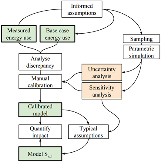
Figure 1. Modeling, calibration, and analysis process.

Case Study Buildings

Four case study buildings were investigated; two university buildings (referred to as CH and MPEB) and two office buildings (referred to as Office 17 and Office 71), all are located in London, the United Kingdom. Access was provided by University College London (UCL) estates and BuroHappold Engineering, both parties were directly involved with this research. The buildings consist primarily of open-plan office space, where both university buildings include some teaching spaces and MPEB includes workshops and laboratories, in addition to two large server rooms. Office 17 is a naturally ventilated building with a provision for air conditioning in the basement and reception. CH and Office 71 are also naturally ventilated, but have air conditioning throughout the building. MPEB has a variety of mechanical systems in place to provide ventilation and air conditioning, in addition to openable windows for natural ventilation in perimeter spaces. Buildings were selected based on their accessibility and availability of both design and measured data at a high level of granularity.

Modeling

Ideally a design model would be available as a starting point, this would allow comparing initial assumptions with a calibrated model, however these are often not available as these are generally not disclosed by the design engineer. Instead models were built based on drawings and specifications in Operation and Maintenance (O&M) manuals. All building spaces were included in the model and zoning of the spaces was identified during walk-throughs of the buildings. OpenStudio¹ (1.14) was used to develop the models, a graphical interface for the EnergyPlus² (8.6) simulation engine. A visualization of the three dimensional virtual models is shown in Figure 2.

FIGURE 2

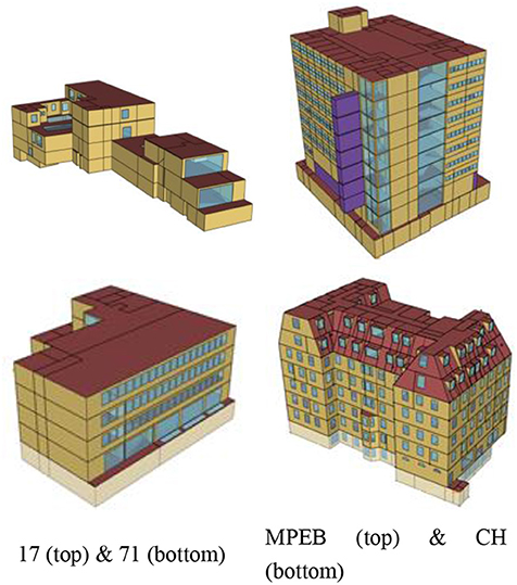
Figure 2. Virtual models of the case study buildings.

Analysis of Discrepancy

Differences between predicted and measured energy use were compared on a detailed level to identify performance issues. Maile et al. (2012) use data graphs to explain performance issues by comparing predicted and measured data. They and others (Yang and Becerik-Gerber, 2015; Chaudhary et al., 2016; Kim and Park, 2016; Sun et al., 2016; Kim et al., 2017) use statistical variables proposed by Bou-Saada and Haberl (1995), such as the normalized mean bias error and CV(RMSE) given in Equations (1) and (2).

$\begin{array}{ll}NMBE(\%)=\frac{\frac{{\displaystyle {\sum }_{i-1}^n}(m_i-s_i)}{n}}{\overline{m}}·100& (1)\end{array}$

$\begin{array}{ll}CV(RMSE)(\%)=\frac{{\left[\frac{{\displaystyle {\sum }_{i-1}^n}{(m_i-s_i)}^2}{n}\right]}^{\frac{1}{2}}}{\overline{m}}·100& (2)\end{array}$

where m_i and s_i are the measured and simulated data points, $\overline{m}$ is the average of the measured time series data and n is the number of data points in the time series (i.e., N_monthly = 12, N_hourly = 8760).

Sampling

For the purpose of uncertainty and sensitivity analysis, variability was introduced to a large set of input parameters in the building models. The Monte Carlo method was employed to repeatedly random sample distributions of inputs to obtain the distribution of energy consumption. The amount of simulations to be run is dependent on when convergence criteria are met, i.e., when the true mean is established. The convergence of the method is based on the size of the sample, which thus determines the computational cost. The sample size is in effect the number of different combinations of input parameters that are run through the deterministic model, whereas the number of parameters included in the sample determine the volume of the parameter input space. The sample sizes were between 100 and 300 variable inputs for the four case study buildings. Including uncertainty in material properties, power densities, scheduling, set-point temperatures, natural and mechanical ventilation requirements, infiltration, and system efficiencies. In this research, Latin hypercube sampling is used for creating randomized designs, which is one of the sampling methods that has been found to have the fastest convergence on the mean estimates (Burhenne et al., 2011). Parameter ranges were established at a 20% variation for all considered variables used in the samples, to allow for enough variation and understand parameter influences as done by Eisenhower et al. (2011).

Parametric Simulation

Each sample of inputs is used to generate separate simulation files, which were then simulated using EnergyPlus on Legion, UCL's computer cluster. For each building, several thousand simulations were run in order to analyse the variance in predictions. A higher number of simulations increase the accuracy of the calculated correlations between inputs and outputs from sensitivity analysis. For sampling, use is made of pyDOE (2017), an experimental design package for Python, with which Latin-hypercube designs were created.

Uncertainty and Sensitivity Analysis

Uncertainty analysis quantifies uncertainty in the output of the model due to the uncertainty in the input parameters. Uncertainty analysis is typically accompanied by sensitivity analysis, which apportions the uncertainty of the model output to the input.

Spearman's rank correlation coefficient (SRCC) was calculated to assess the relationship between the inputs and outputs. SRCC was used in conjunction with Pearson correlation coefficients, but were found to be similar, due to the inputs and outputs being elliptically distributed, as such, only SRCC is shown. Equations for the computed coefficients are as follows:

$\begin{array}{ll}(SRCC){\rho }_{r{g}_X{,rg}_Y}=\frac{cov(r{g}_X,r{g}_Y)}{{\sigma }_{r{g}_X}{\sigma }_{r{g}_Y}}& (3)\end{array}$

where ρ is the correlation.

Manual Calibration

Input parameters are predominantly based on evidenced information collected from O&M manuals and verified in operation through energy audits. In addition, system performance, occupancy presence and energy use is verified through measurements, where energy use is the objective of the calibration process. However, in certain cases, changes made to a model can seem arbitrary when not enough data is available to justify making a change to the model. For example, when over prediction of power energy use is identified, there are then several options for changing the model to align to the actual situation, as power energy use is determined by multiple input parameters in a model. There is no premise for changing one parameter over the other when detailed measurements are not available, even though they will affect the model in different ways. Changing equipment power density in one space with space conditioning opposed to one without will have different effects on heating and cooling loads, whilst achieving the purpose of aligning power energy use. Under this rationale, it becomes clear that a higher level of data granularity can support in developing a more accurate model, but that a lack of information can cause these parameter changes and mask the real situation. Choices made in changing input parameters are not extensively described, but will be explained when significant changes were necessary or when certain limitations were identified that could drastically affect the accuracy of the model.

As such, instead of running through each iteration per model, an overview is given of essential adjustments that were necessary and had a major impact on the accuracy of the model. In addition, limitations are described that were likely to affect model calibration accuracy, typically due to a lack of information.

Results and Discussion

Initial base case models for the case study buildings were created, assumptions were based on collected data from O&M manuals and the Building Management System (BMS) and Automatic Meter Reading (AMR) system. In addition, Wi-Fi and swipe-card access data were collected to inform occupancy presence. Subsequently, uncertainty was introduced to input parameters in order to quantify the uncertainty within the outputs and compute the sensitivity of parameters. This supported the calibration of the base case models toward measured energy use and understanding of the impact of underlying causes of the regulatory performance gap. Several iterations were necessary to adjust the models to achieve a closer representation of the existing building. Manual calibration focused on removing modeling errors and discrepancies between predictions and measurements. More specifically, this involved determining specific holidays in the measured data, establishing base electricity loads for lighting and equipment, disaggregating energy end-uses for juxtaposition, determining systems set-up and HVAC strategy, and introducing seasonal occupancy factors.

Operational Data to Inform Model Assumptions

Collected data is invaluable in supporting assumptions in the building modeling process. In particular, the development of occupancy, equipment, and lighting schedules is essential for model calibration and should even be useable in a design setting, by collecting an evidence base of similar building types and their typical schedules of use. Although environmental and system performance data was also analyzed to establish system settings and set-point temperatures, these variables are much more case study dependent.

Developing Typical Schedules of Use

Lighting and equipment use and occupancy presence in building simulation are based on schedules of use, represented using values between 0 and 1. These schedules are then applied to certain spaces or space types, which are then multiplied by power and lighting loads (W/m²) or occupant densities (m²/p) assigned to these spaces, to calculate the final load (W) or number of people in a space at a certain time of the day. For compliance modeling in the UK, standard schedules are used, which may not be representative of reality. Schedules of use directly affect energy use and can have a large impact on the discrepancy between predicted and measured energy use. As such, for performance modeling during design, it is essential to determine future use of spaces, potentially based on previous experience or data from existing buildings. Operational data can be utilized to develop these schedules of use, either based on; (1) measured occupancy presence data or (2) measured electricity use.

Logically, the use of lighting- and equipment electricity consumption will create more accurate lighting- and equipment use schedules, while occupancy data will create more accurate occupancy presence schedules. The use of occupancy data to represent lighting- and equipment schedules assumes that occupancy presence has a large influence on these types of energy use. Although generally true for most buildings, it can differ per building and is not always as strongly correlated, introducing a certain margin of error. Lighting- and equipment schedules are more important than occupancy schedules as they have a more significant influence on energy use. Using this reasoning, the use of electricity data to develop operational schedules would be the preferred option. Nevertheless, in both cases, it needs to be ensured that the developed schedules do not apply for all space types (depending on the granularity of data collected; whole building/floor/space). Using whole building collected occupancy data would be a better proxy for the schedules of use in office spaces, than in storage-, toilet-, and kitchen spaces. In the case study buildings, the first approach was used for MPEB and CH, where Wi-Fi data was available, but an accurate breakdown of lighting- and equipment electricity was not. Whereas, for Office 17 and 71, solely lighting and equipment electricity data was available and the second approach was used to develop schedules of use.

Schedules Based on Occupancy Data

Swipe card and Wi-Fi data were used to develop typical weekday and weekend day schedules, in particular Wi-Fi was effective at understanding the cumulative trend of people within the building, as shown in Figure 3. Counting the number of swipes gave an indication of the maximum number of people during a day, which was used to define the occupancy density (m²/p) of the different space types.

FIGURE 3

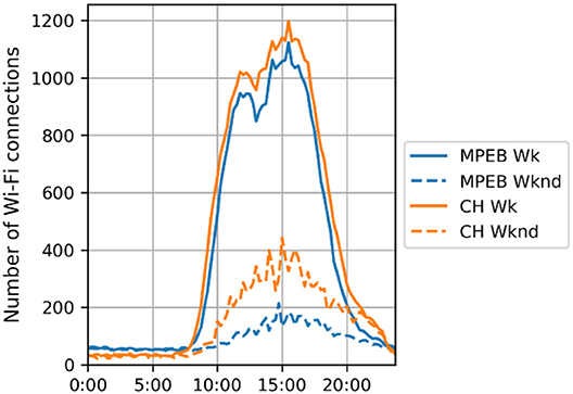
Figure 3. Number of Wi-Fi connections for an average weekday and weekend day at a 15-min interval for CH and MPEB.

The typical profiles were normalized to retrieve values between 0 and 1, to be used as occupancy schedules in the building. However, it became clear that a large variation exists in occupancy throughout the seasons as MPEB and CH are university buildings where occupancy is affected by university terms or semesters, evident from Figure 4.

FIGURE 4

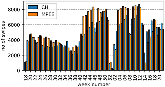
Figure 4. Weekly number of swipe-ins at main entrance in CH and MPEB.

This seasonal variation in occupancy needs to be accounted for in building energy modeling as occupancy has a significant effect on energy use. A monthly seasonal factor was calculated by taking the average daily maximum number of swipes per month. These values were then scaled to between 0 and 1. The seasonal factors were then multiplied by the typical weekday and weekend day schedules, creating a total of 12 different weekday, and weekend day occupancy schedules, one for each month.

It would be possible to incorporate the collected occupancy data directly into the energy modeling software, i.e., instead of creating 12 monthly schedules, each half-hour can be represented by the collected data. This would, however, make the occupancy schedule considerably long, and would over-fit the model, therefore, would only apply to a specific year. Instead, the schedules can take into account uncertainty within the data to understand the effect of variability in the schedules on energy use.

The occupancy schedules were then used to create lighting and equipment schedules by introducing an out-of-hours baseload, which is the lighting or equipment electricity use during unoccupied hours relative to the average peak during the day. This requires making an assumption about the typical baseloads for lighting and equipment use. By analyzing their electricity profiles for the case study buildings, it was found that lighting and equipment energy use baseloads for Office 17, Office 71, CH, and MPEB which were; 20/25, 15/20, 20/65, and 65/85%, respectively. These figures indicate the use of lighting and equipment in the buildings outside of normal operating conditions (night-time operation) as a percentage of total. These figures were used to create the lighting and equipment schedules, by taking the occupancy schedules, and applying the baseload where the occupancy schedule factor is lower than the baseload. Internally, they are multiplied by the assumed lighting and equipment power densities. The resulting occupancy-, equipment- and lighting schedule for a typical weekday and weekend day in CH are shown in Figure 5. It was assumed here that the lighting and equipment schedules are slightly wider than the occupancy schedule. A monthly seasonal factor based on the variation of occupancy was applied to these schedules.

FIGURE 5

Figure 5. Occupancy, equipment, and lighting schedules for a single parametric simulation run for CH.

Schedules Based on Electricity Data

In many buildings, the availability of occupancy data is minimal and assumptions have to be made. To support these assumptions, it might be useful to base occupancy profiles on other available data, such as electricity use. This would ideally require at least a breakdown into lighting and power for the building. For Office 17 and 71, equipment and lighting electricity use was disaggregated and available per floor. Absolute electricity use schedules were scaled to between 0 and 1, as to be used in the building simulation software. Either separate schedules can be used for each floor (as shown in Figure 6) or an average for the building can be calculated.

FIGURE 6

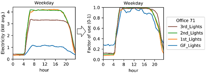
Figure 6. Lighting electricity use per floor scaled to between 0 and 1.

There is often a strong correlation between lighting and power energy use and occupancy, indicating that they follow a similar trend. However, their main difference is the baseload in electricity use (i.e., night-time energy use), which is not the same for occupancy. To create occupancy profiles solely based on the lighting and power electricity use, the L&P profiles were first scaled to between 0 and 1, the baseload is then subtracted from the values in the time series and negative values are set to 0. Then, the time series is again scaled to between 0 and 1, and a typical weekday and weekend day were calculated, as shown in Figure 7.

FIGURE 7

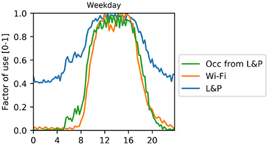
Figure 7. Weekday occupancy profile based on L&P electricity use, for CH.

As can be seen, the newly created occupancy profile, solely based on lighting and power electricity, represent the actual Wi-Fi data well. However, the accuracy of this method is strongly dependent on the assumed baseload.

Sensitivity Analysis

For each model, parametric simulations created an input- and output space (i.e., samples of input parameters and predictions of energy use). Predictions were aggregated by comparable end-uses, to create a like-for-like comparison with measurements. In Figure 8, energy end-uses for 3,000 simulations are compared with measured energy use (orange circles), displaying the uncertainty for each end-use.

FIGURE 8

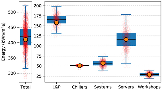
Figure 8. Predicted (blue) and measured (orange) energy use for 3,000 simulations for MPEB.

By varying the input parameters within the model, their individual impact on different end-uses can be analyzed. For example, varying the space set-point temperature deadband or L&P profiles during different simulations, can highlight how these impact cooling energy use, as shown in Figure 9. A change in deadband would have a larger influence on cooling energy use than offsetting the L&P profiles.

FIGURE 9

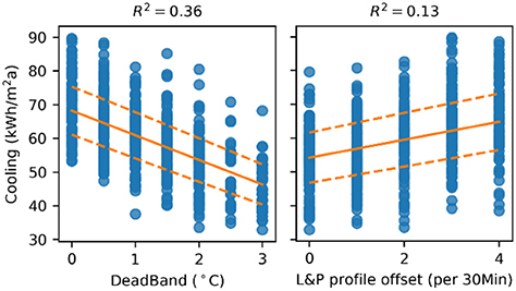
Figure 9. Impact of varying the space set-point deadband and lighting and power profiles of use on cooling energy use.

The inputs and outputs were used to understand the sensitivity of the input parameters on the outputs.

CH

For CH, the variability in “DeadBand” (i.e., interval between heating and cooling temperature) has a strong negative correlation (ρ = −0.6) with cooling energy use. This can be seen in Figure 10, where input variables are filtered where ρ >[dolmath] ±0.25 for any of the energy end-uses.

FIGURE 10

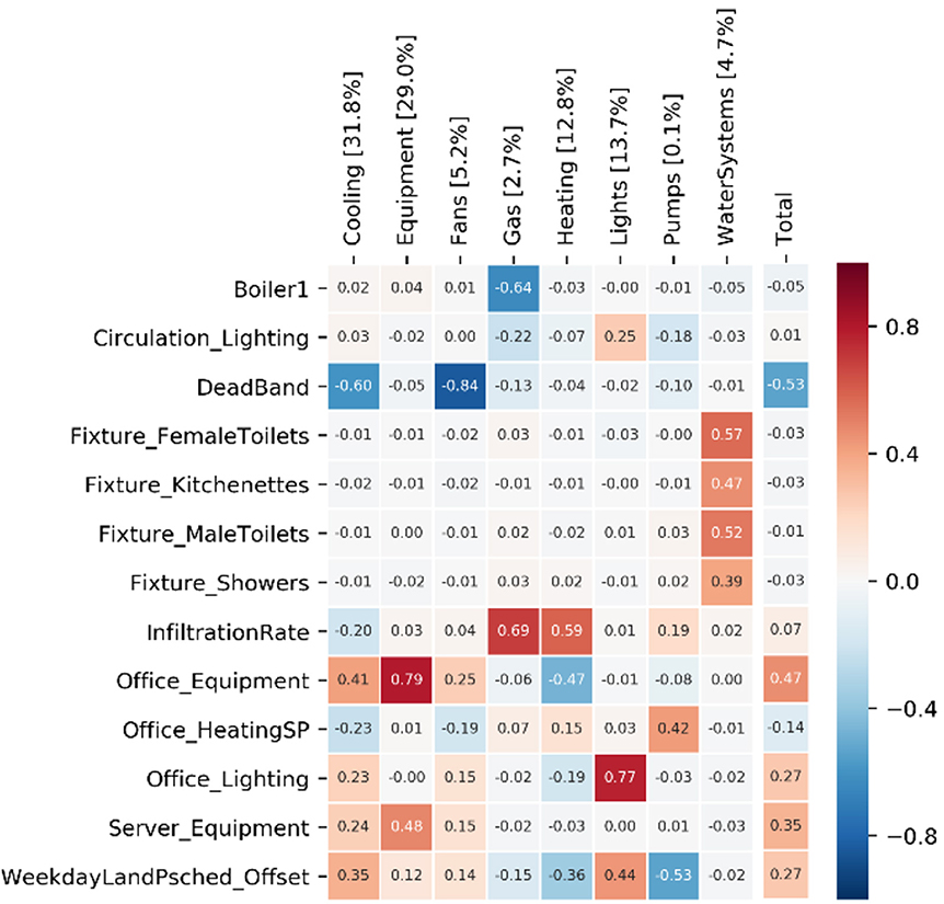
Figure 10. Spearman correlation coefficient per energy end-use and total energy use for CH.

Set-point temperatures were varied at a 0–3°C interval. This was primarily helpful to capture the uncertainty of the Variable Refrigerant Flow (VRF) control strategy. In addition, equipment power density, as defined for the office spaces, has a strong positive correlation (ρ = 0.79). Other parameters, such as the boiler efficiency have a strong negative correlation (ρ = −0.64) with gas use, i.e., an increase in the boiler efficiency reduces gas energy use. Although, some of these parameters have a strong correlation with individual end-uses, their effect on total energy is negligible, as presented on the right side of the diagram. For example, boiler efficiency is weakly correlated to total energy use, because of the small percentage of gas use out of total energy use, used solely for radiator heating within circulation spaces. The “weekday L&P offset” refers to the variability introduced by allowing the lighting and power schedules to fluctuate by up to 2 h as a horizontal offset.

Office 17

For Office 17, significant parameters are the lighting and equipment power densities, typical for office buildings that are naturally ventilated. They have a strong positive correlation (Lights ρ = 0.36, Equipment ρ = 0.90) on electricity use and coincidentally a strong negative correlation (Lights ρ = −0.23, Equipment ρ = −0.41) on gas use, due to an increase in internal gains, which decreases the need for radiator heating (the only form of mechanical heating). Furthermore, gas use is strongly dependent on the heating temperature and allowance for opening windows, increasing either will have a strong effect on increasing gas energy use.

Office 71

For Office 71, the strongest positive correlation (ρ = 0.97) is between the mechanical outdoor air flow rate to the offices and fan energy use. This input was sampled with a mean (μ) of 8 and standard deviation (σ) of 1.2 l per second. In contrast, the strongest negative correlation is between the hot water temperature of the boiler (μ = 82, σ = 4) and the pump energy use. Although both highlight strong effects on their respective energy end-uses, their proportionate effect on total energy use is considerably smaller. Instead, most important variables are lighting and equipment power density.

MPEB

For MPEB there are a multitude of parameters that affect different energy end-uses. In particular, lighting and equipment power densities in the offices, servers, and laboratories have a strong positive correlation on lighting and equipment (including server) energy use. These in turn affect the correlation coefficients of the VRF heat pump Cooling Coefficient of Performance (CCOP), which has a strong positive correlation (ρ = 0.35) on systems energy use. However, on total energy use, the server equipment power density (i.e., W/m² produced by computer clusters) is the dominant factor with a very strong positive correlation (ρ = 0.92). In addition, it strongly influences chiller (ρ = 0.45), fan (ρ = 0.98), pumps (ρ = 0.98), and systems energy use (ρ = 0.9). Systems energy use in MPEB is mainly from the VRF heat pump, providing cooling in the server rooms. Whereas, chillers energy use is from the chillers, providing cooling to both Fan Coil Units (FCUs) in the server rooms and offices, in addition to the air handlers, providing conditioning to occupied spaces. Server energy use in the building is 1/5th of total energy use, but the sensitivity indices show that other energy end-uses are strongly affected due to the high cooling loads and necessary conditioning.

Summary

Spearman rank correlation coefficients for each building are summarized in Table 1, in order of significance. In particular, equipment power density is a significant parameter to influence energy use, which is typical for non-domestic buildings. Therefore, it is important to make evidence based assumptions about these loads to make sure predictions are in line with measurements. It is important to note that both equipment and server energy use are not taken into account under the current regulatory framework. Other significant factors to influence energy use in the case study buildings are the heating and cooling set points, in particular in spaces with high internal gains, where temperatures can strongly fluctuate. Insignificant parameters to influence energy use are material properties and air infiltration. For domestic buildings, the thermal envelope has a considerable impact on reducing heating energy use (in colder climates). In contrast, in non-domestic buildings, an increase of the performance of the thermal envelope can have a negative effect on energy use due to high internal gains in certain spaces, which inhibit heat loss to the outside, and therefore, have an increased cooling load. In high-density workspace in modern buildings, Passive house standard envelopes are therefore unlikely to be an energy efficient design decision. Similarly, infiltration does not have a significant effect on energy use in any of the buildings, although there is a distinct difference between the seasons.

TABLE 1

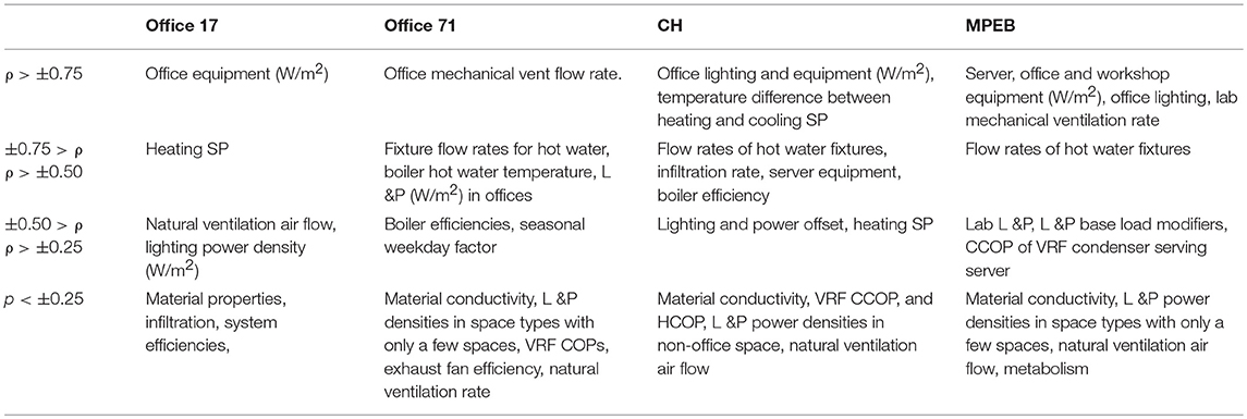
Table 1. Spearman correlation coefficients of input parameters on total energy use per building.

Calibration

For each building model, manual adjustments were made to bring the predicted energy use closer to measured energy use (i.e., manual calibration). O&M manuals were to be reviewed to understand the design and intended operation of a building, which were subsequently validated through energy audits. The latter is especially important, as the intended design and design strategies differed from that observed, which in many cases had a significant effect on energy performance. An overview is given of typical adjustments among the case study buildings, and more specific adjustments to adjust outliers.

Specific Adjustments

• For both Office 17 and 71, the boiler is turned off during the summer months (May to September). However, according to the simulation model, some heating is necessary during these months (based on the weather). To replicate reality, the boiler was turned off in the model.

• Continuous operation of the VRF system during day and night in CH was identified. This was represented by adjusting night-time heating- and cooling set-points. Whereas, for MPEB, continuous chillers use was measured, mainly due to the high continuous load from high-performance computing clusters.

• In Office 17, gas use during the night was similar to its daytime baseload, different from initial assumptions. To represent this in the model, the boiler was configured to provide heating during the night. After communicating this issue to facilities management, the boiler was set to operate on a timer. Consumption drastically decreased as a result, as can be seen in Figure 11, where gas use for two typical weekdays for the winter of 2013 and 2016 are shown.

• In addition, seasonality in occupancy presence proved to be a major factor of variability for the university buildings. This was represented by introducing a seasonality factor for occupancy, lighting and equipment loads, calculated by analyzing the occupancy (Wi-Fi and swipe-card data), lighting and power loads throughout the seasons.

FIGURE 11

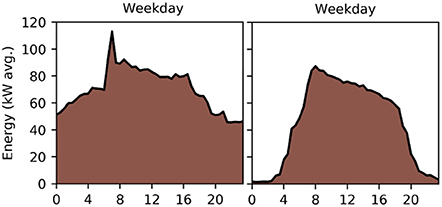
Figure 11. Gas energy use for an average weekday during January to April 2013 (Left) and 2016 (Right).

Typical Adjustments

• Another example that caused differences between predictions and measurements is the occurrence of holidays, which a model needs to take into account. Although this is standardized within the NCM methodology, for performance modeling purposes, this needs to be explicitly defined in the model.

• For each building, the out of hours equipment and lighting baseloads were important factors, determined by calculating typical weekday and weekend day profiles and comparing their peak and base-loads, specifically for lighting and power where available. The power baseloads were defined as 20, 20, 85, and 65% for Office 17, Office 71, MPEB, and CH, respectively.

Limitations

Limitations were identified that resulted in some uncertainty within the calibrated models, in particular these were related to the following:

• Metering systems did not always pick up all end-uses accurately, due to mislabeling, faulty meters, and some systems not being measured. In particular, for Office 71, the VRF system and AHU were not metered, and calibration was performed solely on the other available end-uses. Similarly in MPEB, the heat meter for the district heating system was out of order.

• Electric water heating (through zip-taps and showers) cannot be distinguished from measured power energy use (i.e., plug loads). Therefore, this use was added to the power use within the models ensuring a like-for-like comparison.

• Electricity use for heating and cooling provided by VRF systems cannot be separated as is normally done for building simulation. These are therefore combined.

• Related to a previous bullet point, a VRF system with local set-point control is difficult to represent in building simulation, and will introduce some uncertainty within the calibration.

• For MPEB, part of the server electricity use was determined to be connected to the L&P bus-bar, making it impossible to distinguish these loads accurately.

These limitations are a common issue with model calibration, however, most could be alleviated through rigorous and continuous commissioning, in addition to ensuring that a reliable metering strategy is in place.

All four case study buildings were calibrated within the ASHRAE criteria at a monthly level as shown in Table 2. At an hourly level however, both Office 17 and 71 show significant differences due to discrepancies between predicted and measured gas use. In both buildings, heating was turned off manually for the summer months. In contrast, the model still predicted significant gas use. Additionally, there was significant night-time gas use (heating during the night), which was not fully taken into account in the model. Together, this resulted in large differences at an hourly level.

TABLE 2

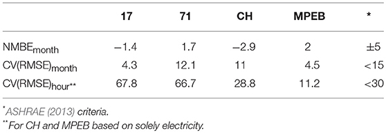
Table 2. Statistical calibration criteria, differences between predicted and measured energy use.

The ASHRAE criteria are helpful to understand differences between predicted and measured energy use, but provide a limited understanding of differences at a higher temporal granularity, in particular for the NMBE, a statistic where negative and positive values can cancel each other out. As such, comparison of the NMBE and CV (RMSE) at different energy end-uses on a monthly basis were also made. Aggregated electricity use is shown for MPEB in Figure 12.

FIGURE 12

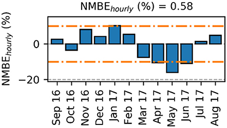
Figure 12. NMBE based on hourly electricity³.

Furthermore, the ASHRAE calibration criteria are for total energy use, and do not take into account the differences between energy end-uses. One end-use can potentially mask the other. To avoid this, calibration focused on limiting differences between end-uses where a like-for-like comparison was possible. Comparing typical weekday and weekend day for predicted and measured energy use proved to be helpful in determining typical hourly differences and identified if adjustments were necessary. For example, as shown in Figure 13, system and L&P energy use for a typical day indicates that: (1) electricity is under predicted for the system, while the profile is a good approximation of its variability, and (2) the assumed total power density of lighting and power should be slightly lower to align with the measured profile.

FIGURE 13

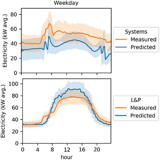
Figure 13. Typical weekday Systems and L&P electricity use for CH.

Impact of Regulatory Assumptions

To determine the impact of regulatory assumptions on energy use predictions and consequently the performance gap, typical NCM assumptions (i.e., simplifications) were applied to the manually calibrated base case models. Simplifications were applied both individually and combined to understand their individual and aggregated effect on energy use. An overview of the applied simplifications is given in Table 3.

TABLE 3

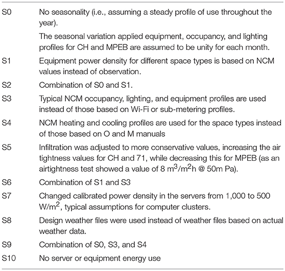
Table 3. Simplifications.

Input variables, such as material properties, system efficiencies, metabolism, and natural ventilation rates, have not been further investigated as these were shown to be least impactful by the sensitivity analysis. Simplifications were applied to base case models for each case study building, however several simplifications were not applied to each building as they were not initially taken into account, such as the seasonality in Office 17 and 71. The percentage impact on total energy use for each simplification is shown in Table 4.

TABLE 4

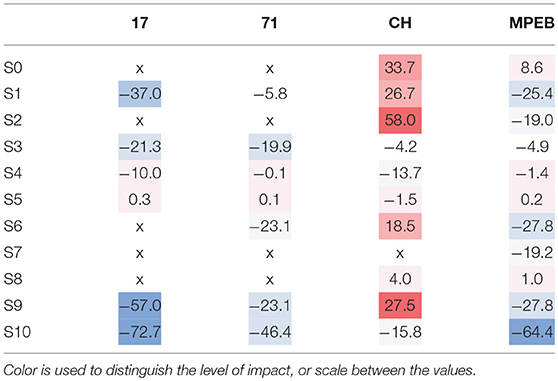
Table 4. Percentage impact of simplifications on total energy use compared to the calibrated model.

Simplifications concerned with a change of internal gains highlight the importance of accurately determining the assumptions for equipment and lighting power density in spaces, as they have a large effect on total energy use. This is supported by the strong correlation coefficients for these parameters. In particular, server loads can be dominant in modern buildings, evident for MPEB where energy use in the building was primarily driven by the power use of the computer clusters, indirectly influencing systems' electricity use. Moreover, defining the right schedules for these loads is tantamount to establishing the right loads for spaces. Its effect was significant on energy use for each of the case study buildings, as shown by S1 and S3. In particular, a significant difference is notable for S1 between MPEB and CH, which is due to the difference between the NCM and calibration assumptions for equipment power density. More specifically, it was found to be directly related to the power density of the server rooms, which for CH, was half of that of the NCM assumption (500 W/m²), where it was double that in MPEB.

As part of the manual calibration process, it was found that high baseloads existed in the buildings, which had to be accounted for by adjusting the internal gain schedules. These were a large contributor to a discrepancy between regulatory predictions and measurements as there was a significant difference compared to the typically assumed NCM equipment power baseload. In the case study buildings, the baseloads for equipment in Office 17, 71, CH and MPEB were ~25, 20, 65, 85%, respectively, compared to the NCM assumption of 5.3%. NCM and calibrated model schedules of use are shown for CH in Figure 14, which clarify the cause of their significant impact.

FIGURE 14

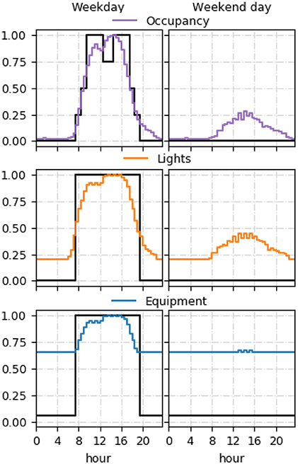
Figure 14. Occupancy, lights, and equipment schedules for the calibrated model compared with NCM (in black) assumptions for CH.

Besides internal gains, the heating and cooling temperatures in different space types can vary significantly between initial assumptions and those in operation, something which is difficult to replicate within a model when a variable strategy is in place. In CH in particular, the operational set-point temperatures could be adjusted manually by occupants and this was difficult to replicate accurately, especially since system energy use for conditioning was found to be constant in both CH from the VRF system and MPEB from the chillers. Replacing the calibrated set-point temperatures with NCM assumptions led to a significant decrease in energy use for Office 17 and CH, while for Office 71, the temperatures were similar to NCM assumptions. Finally, for S8, changing the weather file based on actual historical weather data to a design weather file from Gatwick had a notable effect in increasing annual energy use for CH (4%), but only a minor effect for MPEB (1%). This is in contrast to some earlier findings that have shown differences of up to 7% on annual energy (Bhandari et al., 2012).

Conclusion

Discrepancies between predicted and measured energy use was mitigated through iterative adjustment of building energy model assumptions in four case study buildings. The reliability of this process is strongly dependent on the availability of both design and measured data, which is the evidence to support any iterative changes. If there is a lack of such data, any iterative changes will be arbitrary, even though a discrepancy may be mitigated. Under this rationale, it becomes clear that a higher level of data granularity supports the development of a more accurate model. A higher level of data granularity and availability of evidence can filter out inaccurate predictions.

Calibrated models were used to quantify the impact of regulatory design assumptions on energy use. Regulatory assumptions are those defined under the UK National Calculation Methodology, which pre-scribe the inputs for specific space types, in order to determine the minimum performance requirements of a building for Building Regulations (i.e., compliance modeling). Compliance modeling should not be used as a design tool by informing building efficiency improvements. In practice, however, this occurs as increasingly stringent building efficiency targets set by the government or local councils are not being met. Further refinement of the design is necessary to achieve these targets, which may be tested through the compliance model, even though the compliance model is not an actual representation of the building. Tested efficiency measures can have a significantly different impact on the compliance model than on the actual building.

The impact of typical assumptions on energy use identified the significant differences that exist between regulatory assumptions and the actual operation of a building, giving a better understanding of how and what assumptions should be made when using performance modeling. The findings underline the need to confirm, most importantly; future equipment loads, equipment and lighting (or occupancy) schedules, seasonality of use, and heating and cooling strategies of a building. In addition, typical lighting and equipment baseloads under compliance modeling are a gross under-prediction of actual baseloads measured in the four case study buildings.

The use of operational data to inform assumptions for modeling existing buildings is straightforward, but may also prove to be worthwhile during the design of new buildings. Data on similar buildings, predominantly based on building type, can be used as a proxy for design stage building energy models; (1) indirectly, input parameters as identified in this paper can be applicable to certain new buildings, and (2) directly, by collecting data on existing buildings, in particular, understanding those significant variables as identified by the sensitivity analysis; plug loads, profiles of use (incl. baseloads), domestic hot water use and server loads.

This paper highlights that a stronger emphasis on the use of performance modeling is needed, in order to drive design decisions that will effectively mitigate the risk of the energy performance gap.

Author Contributions

CvD, the main author, is a doctoral researcher and is the main contributor to this original research paper. MD is CvD's industrial supervisor during his doctoral studies. EB is CvD's academic supervisor during his doctoral studies and has reviewed the paper and provided feedback on the work, including direct insights from his own work. CS is CvD's secondary academic supervisor during his doctoral studies. DM is CvD's first academic supervisor during his doctoral studies and has reviewed the paper and provided feedback for initial revision. DM is an Associate Editor for the HVAC Journal.

Conflict of Interest Statement

The main author was sponsored by BuroHappold Engineering to carry out this research, supervised by MD employed at BuroHappold Engineering. BuroHappold Engineering had no role in study design, data collection, data analysis, decision to publish or preparation of the manuscript.

The remaining authors declare that the research was conducted in the absence of any commercial or financial relationships that could be construed as a potential conflict of interest.

Acknowledgments

This research has been made possible through funding provided by the Engineering and Physical Sciences Research Council (EPSRC) and BuroHappold Engineering, under award reference number 1342018.

Footnotes

1. ^https://www.openstudio.net/

2. ^https://energyplus.net/

3. ^See Appendix for further explanation.

References

ASHRAE, (2013). ASHRAE Fundamentals. Atlanta, GA: ASHRAE.

Bhandari, M., Shrestha, S., and New, J. (2012). Evaluation of weather datasets for building energy simulation. Energy Build. 49, 109–118. doi: 10.1016/j.enbuild.2012.01.033

CrossRef Full Text | Google Scholar

Bou-Saada, T., and Haberl, J. (1995). An Improved Procedure for Developing Calibrated Hourly Simulation Models. Montreal, QC: IBPSA Proceedings.

Google Scholar

Burhenne, S., Jacob, D., and Henze, G. (2011). “Sampling based on sobol' sequences for monte carlo techniques applied to building simulations,” in: 12th Conference of International Building Performance Simulation Association (Sydney, NSW).

Google Scholar

Chaudhary, G., New, J. R., Sanyal, J., Im, P., O'Neill, Z., and Garg, V. (2016). Evaluation of “Autotune” calibration against manual calibration of building energy models. Appl. Energy 182, 115–134. doi: 10.1016/j.apenergy.2016.08.073

CrossRef Full Text | Google Scholar

Clarke, J. (2001). Energy Simulation in Building Design, 2nd Edn, s.l. Glasgow: Butteworth Heinemann.

Google Scholar

Construction Task Force (1998). Rethinking Construction. London: Department of the Environment, Transport and the Regions.

Cox, A., and Townsend, M. (1997). Latham as half way house: a relational competence approach to better practice in construction procurement. Eng. Constr. Arch. Manage. 4, 143–158. doi: 10.1108/eb021045

CrossRef Full Text | Google Scholar

Diamond, R., Berkeley, L., and Hicks, T. (2006). “Evaluating the energy performance of the first generation of LEED-certified commerical buildings,” in Proceedings of the 2006 American Council for an Energy-Efficient Economy Summer Study on Energy Efficiency in Buildings (Berkeley, CA).

Google Scholar

Eisenhower, B., O'Neill, Z., Fonoberov, V., and Mezic, I. (2011). Uncertainty and sensitivity decomposition of building energy models. J. Build. Perform. Simul. 5, 171–184. doi: 10.1080/19401493.2010.549964

CrossRef Full Text | Google Scholar

Fabrizio, E., and Monetti, V. (2015). Methodologies and advancements in the calibration of building energy models. Energies 8, 2548–2574. doi: 10.3390/en8042548

CrossRef Full Text | Google Scholar

House of Commons, (2008). Construction Matters - Ninth Report of Session 2007-08 Vol. 1. London: The Stationery Office Limited.

Kim, Y., Heidarinejad, M., Dahlhausen, M., and Srebric, J. (2017). Building energy model calibration with schedules derived from electricity use data. Appl. Energy 190, 997–1007. doi: 10.1016/j.apenergy.2016.12.167

CrossRef Full Text | Google Scholar

Kim, Y., and Park, C. (2016). Stepwise deterministic and stochastic calibration of an energy simulation model for an existing building. Energy Build. 133, 455–468. doi: 10.1016/j.enbuild.2016.10.009

CrossRef Full Text | Google Scholar

Maile, T., Bazjanac, V., and Fischer, M. (2012). A method to compare simulated and measured data to assess building energy performance. Build. Environ. 56, 241–251. doi: 10.1016/j.buildenv.2012.03.012

CrossRef Full Text | Google Scholar

NCM, (2013). National Calculation Methodology (NCM) Modelling Guide (for Buildings Other than Dwellings in England). London: Department for Communities and local Government.

Norford, L., Socolow, R., Hsieh, E., and Spadaro, G. (1994). Two-to-one discrepancy between measured and predicted performance of a ’low-energy’ office building: insights from a reconciliation based on the DOE-2 model. Energy Build. 21, 121–131. doi: 10.1016/0378-7788(94)90005-1

CrossRef Full Text | Google Scholar

Pan, Y., Huang, Z., and Wu, G. (2007). Calibrated building energy simulation and its application in a high-rise commercial building in Shanghai. Energy Build. 39, 651–657. doi: 10.1016/j.enbuild.2006.09.013

CrossRef Full Text | Google Scholar

pyDOE (2017). pyDOE Design of Experiments for Python. Available online at: https://pythonhosted.org/pyDOE/ (accessed July 20, 2018).

Raftery, P., Keane, M., and O'Donnell, J. (2011). Calibrating whole building energy models: an evidence-based methodology. Energy Build. 43, 2356–2364. doi: 10.1016/j.enbuild.2011.05.020

CrossRef Full Text | Google Scholar

Sun, K., Hong, T., Taylor-Lange, S., and Piette, M. (2016). A pattern-based automated approach to building energy model calibration. Appl. Energy 165, 214–224. doi: 10.1016/j.apenergy.2015.12.026

CrossRef Full Text | Google Scholar

Torcellini, P., Pless, S., Deru, M., Griffith, B., Long, N., and Judkoff, R. (2006). Lessons Learned From Field Evaluation of Six High-Performance Buildings. Pacific Grove, CA: ACEEE Summer Study on Energy Efficiency in Buildings. doi: 10.2172/884978

CrossRef Full Text | Google Scholar

Turner, C., and Frankel, M. (2008). Energy Performance of LEED for New Construction Buildings. Washington, DC: New Buildings Institute.

Google Scholar

van Dronkelaar, C., Dowson, M., Spataru, C., and Mumovic, D. (2016). A review of the regulatory performance gap and its underlying causes in non-domestic buildings. Front. Mech. Eng. 1:17. doi: 10.3389/fmech.2015.00017

CrossRef Full Text | Google Scholar

Yang, Z., and Becerik-Gerber, B. (2015). A model calibration framework for simultaneous multi-level building energy simulation. Appl. Energy 149, 415–431. doi: 10.1016/j.apenergy.2015.03.048

CrossRef Full Text | Google Scholar

Appendix

Data Visualization and Analysis Techniques

Several visualizations were used that might not be straightforward to understand and are therefore explained here, to be used as a reference.

“Typical” Weekday and Weekend Day Profiles

Typical weekday and weekend day profiles of energy use were used to compare predicted and measured energy use and understand the hourly variation in energy use, profiles were created for a per year basis. A typical weekday and weekend day are determined by first separating the holidays, working days and weekend days in a specific time series (these are year dependent). The separated day types are then grouped together and the average, mean, standard deviation during a specific period is determined. The mean represents a typical day and is in some instances accompanied by the standard deviation throughout the same period. In addition, in certain cases, the profile is normalised to unity (i.e., scaled to bring the values into the range [0,1]).

Discrepancy Metrics Analysis

A discrepancy between predicted and measured energy use is analysed by using the mean bias error (NMBE) and coefficient of variation of the root mean square error [CV(RMSE)], these metrics indicate the error or difference between two datasets. Used here to indicate the error on a monthly level (differences between energy use on a monthly interval) and hourly level (differences between energy use at an hourly interval). The bar graph in Figure A1 indicates the differences on an hourly interval per month, whereas both metrics can also be calculated on a yearly basis. The difference between two datasets at an hourly interval over the whole year is given by NMBE_hourly and CV(RMSE)_hourly. Differences between the months on a yearly basis are given by NMBE_monthly and CV(RMSE)_monthly. Finally, the orange lines are the criteria set by ASHRAE that deem a model calibrated, however these criteria should actually be compared at a yearly basis (the metrics shown at the top of the graph). They are used in the bar graph to understand how the model is performing on a monthly basis.

FIGURE A1

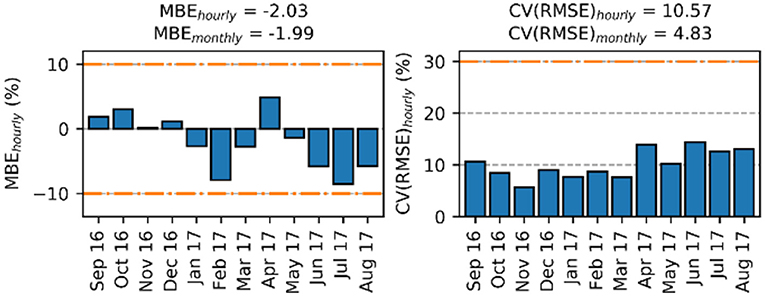
Figure A1. Example of a discrepancy metrics analysis.