Refinement of α-Synuclein Ensembles Against SAXS Data: Comparison of Force Fields and Methods

Introduction

Intrinsically Disordered Proteins (IDPs) play important roles in a wide range of biological processes including cell signaling and regulation (Uversky et al., 2005; Das et al., 2015; Snead and Eliezer, 2019), and their malfunction or aggregation is linked to neurodegenerative diseases such as Alzheimer's and Parkinson's disease. A key, defining property of IDPs is that they do not adopt well-defined, permanent secondary and tertiary structures under native conditions, and their conformational properties are thus best described in statistical terms.

Due to the dynamic nature of IDPs and their inherent conformational heterogeneity, IDPs are not easily amenable to high-resolution characterization solely through experimental measurements. To characterize their structural and dynamic properties it is often necessary to integrate various biophysical experiments, and particularly nuclear magnetic resonance (NMR) spectroscopy (Dyson and Wright, 2001), small angle X-ray scattering (SAXS) (Bernado and Svergun, 2012), circular dichroism (Chemes et al., 2012), and single-molecule Förster resonance energy transfer (sm-FRET) (LeBlanc et al., 2018) have been widely used to characterize the structural properties of IDPs. For instance, pulsed-field-gradient NMR diffusion and SAXS experiments are especially useful to quantify the level of compaction of the IDP. Techniques such as sm-FRET and NMR paramagnetic relaxation enhancement (PRE) provide distance information between different residues or regions of the IDP (Dedmon et al., 2005; Eliezer, 2009). Nevertheless, since most experimental methods only convey ensemble-averaged information and are also affected by random and systematic errors, it is difficult to directly extract information on the underlying heterogeneous ensemble of the IDP. To address this problem, theoretical and computational models can be used to extract detailed structural information from these experiments.

Molecular dynamics (MD) simulations that use physics-based force fields may provide high-resolution temporal and spatial information about the structure and dynamics of IDPs. Extensive sampling of a force field with MD simulations can thus be used to generate conformational ensemble of the IDP. The quality of the results, however, depends heavily on the accuracy of the force field employed. For example, it has been shown that many earlier generations of force fields produce overly compact conformations for many IDPs (Piana et al., 2015). It appears that these force fields fail to accurately describe the solvation of the protein by underestimating protein-water interactions (Sun and Kollman, 1995; Nerenberg et al., 2012; Best et al., 2014; Piana et al., 2015). Recently, however, significant advancements have been made to improve force field accuracy and correct the bias toward overly compact conformations (Best et al., 2014; Piana et al., 2015; Song et al., 2017; Robustelli et al., 2018). Adding to these issues, the large conformational phase space of IDPs, requires extensive sampling of the protein in order to generate converged ensembles. To achieve sufficient sampling, and push the sampling capacity of MD simulations, one often employs enhanced sampling methods such as metadynamics (Barducci et al., 2008) or parallel-tempering replica exchange (Sugita and Okamoto, 1999). Notably, force field and sampling problems are expected to be more severe for longer IDPs.

An approach to address the challenges of force-field accuracy is to combine experimental and theoretical information in order to obtain conformational ensembles of IDPs that agree with experimental measurements. In this way, the simulations are used as a tool to interpret experimental measurements. A number of different approaches have been described and can, roughly, be divided into two different classes in which the experimental data is either (i) used for on-the-fly restraining of a simulation to experimental data, or (ii) post-processing ensembles generated by simulations to match experimental data by reweighting or selection methods. Many different such methods exist, and we refer to recent reviews for additional details (Cesari et al., 2018; Orioli et al., 2020).

Because the conformational ensembles are broad and the experimental data often have low information content and may be noisy, Bayesian inference methods (Box and Tiao, 2011) and the maximum entropy principle (Jaynes, 1957) have emerged as particularly successful frameworks for studying IDPs. In these frameworks, an ensemble generated using a prior model is minimally modified to match the experimentally observed data better. An extension of these frameworks for integrative structural ensemble determination is Metainference Metadynamics (M&M) (Bonomi et al., 2016a), that combines multi-replica all-atom molecular dynamics simulations with ensemble averaged experimental data (Bonomi et al., 2016b). In the M&M approach, the metainference (Bonomi et al., 2016a) part is a Bayesian inference method that allows for the integration of experimental information with prior knowledge of the system from, e.g., physics-based force fields, while also dealing with uncertainty and errors as well as conformationally heterogeneous systems. In addition, metainference can be combined with metadynamics (Laio and Parrinello, 2002; Bonomi et al., 2016b) to accelerate sampling further. A related Maximum Entropy approach has also been applied to determine an ensemble of configurations from SAXS data but using a more refined and potentially accurate method for taking solvent effects into account (Hermann and Hub, 2019). While the above approaches apply the bias on the fly, other Bayesian formalisms takes as input simulations that were generated without taking the experimental data into account, and subsequently updates this using statistical reweighting. Such approaches include our Bayesian/Maximum Entropy (BME) protocol (Bottaro et al., 2020), as well as related methods (Hummer and Köfinger, 2015).

Here, we combined ensemble-averaged experimental SAXS data with MD simulations with the aim to achieve structural ensembles of the system which are in agreement with the experimental data. We did so using both metainference and BME. In particular, we used BME to refine ensembles that had previously been generated using MD simulations (Piana et al., 2015; Robustelli et al., 2018), while metainference was applied to restrain experimental SAXS data during MD simulations with an implicit solvent model (Bottaro et al., 2013). We used the intrinsically disordered protein α-synuclein (αSN) protein as a model, as this protein has been studied extensively by various experimental methods including SAXS and NMR measurements, and because of the availability of long MD trajectories generated from a range of force fields and water models. αSN is a 140-residue long IDP that is primarily expressed in the brain and in its monomeric state is known to be disordered and populate multiple conformational states. αSN aggregation into amyloid fibrils is linked to Parkinson's disease and dementia with Lewy bodies (Spillantini and Goedert, 2000; Ulusoy and Di Monte, 2013).

We assessed the quality of existing ensembles before refinement, and the ability of metainference and BME methods to improve them through incorporation of experimental SAXS data, by comparing with independent measurements of the level of compaction (through the hydrodynamic radius, R_h, as probed by NMR) and previously measured paramagnetic relaxation enhancement data (Dedmon et al., 2005). We find that the inclusion of a SAXS-restraint in the M&M simulation resulted in the generation of a reliable and heterogenous conformational ensemble that also improved the agreement with the NMR diffusion data. The BME reweighting improved the agreement with the experimental data when we applied the approach to simulations with the TIP4P-D water model. For simulations using the TIP3P water model, which were substantially more compact, it was difficult to find a suitably large ensemble compatible with the experimental SAXS data. Together, our result provide insight into how and when experimental SAXS data can be used to refine ensembles of IDPs, and the role played by the force field as a ‘prior’ in these Bayesian/Maximum entropy approaches.

Methods and Materials

Experimental Data

Human αSN for SAXS experiments was expressed, purified, and lyophylized as previously described (van Maarschalkerweerd et al., 2014). Prior to SAXS data collection, the lyophilized powder was dissolved in PBS (20 mM Na₂HPO₄, 150 mM NaCl, pH 7.4) and filtered through a 0.22 μm filter to remove larger aggregates. The final sample concentration before SEC-SAXS was determined by A₂₈₀ to be 4.5 mg/mL using an extinction coefficient of 5960 M⁻¹ cm⁻¹. SAXS data was collected as SEC-SAXS data on beamline P12 (Blanchet et al., 2015) operated by EMBL Hamburg at the PETRA III storage ring (DESY, Hamburg, Germany). 50 μL 4.5 mg/mL αSN in PBS buffer (20 mM Na₂HPO₄, 150 mM NaCl, pH 7.4) was injected on a Superdex 200inc 5/150 GL column with a flowrate of 0.4 mL/min. The column was pre-equilibrated with the running buffer (PBS with 2% (v/v) glycerol). SAXS data were collected at 20 °C, with continuous exposure of 1 s per frame throughout the SEC elution. Data processing was done using CHROMIXS (Panjkovich and Svergun, 2018), averaging sample data from the frames in the monomeric peak and subtracting the buffer signal taken from the flow-through prior to the sample elution to obtain the final scattering profile (Supplementary Figure 1).

We purified αSN for NMR experiments as previously described (Skaanning et al., 2020). Translational diffusion constants for αSN (50μM with 2% (v/v) glycerol) and 1,4-dioxane (0.2% v/v; as internal reference) were determined by fitting peak intensity decay from diffusion ordered spectroscopy experiments (Wu et al., 1995), using the Stejskal-Tanner equation as described (Prestel et al., 2018). Spectra (a total of 64 scans) were obtained over a gradient strength of 2 to 98%, with a diffusion time (Δ) of 200 ms and gradient length (δ) of 3 ms. Diffusion constants were used to estimate the hydrodynamic radius for αSN described (Wilkins et al., 1999; Skaanning et al., 2020) (Supplementary Figure 2).

We used previously measured PRE data obtained by measuring intensity ratios with spin-labels added at five different positions (residue: 24, 42, 62, 87, and 103) (Dedmon et al., 2005).

Bayesian/Maximum Entropy Reweighting of Unbiased MD Simulations

We used previously generated ensembles of αSN obtained by long-timescale MD simulations with different force fields from the CHARMM and Amber families (here abbreviated by C and A, respectively) and water models (Piana et al., 2015; Robustelli et al., 2018) (Table 1). The published simulation using Amber ff99SB-disp (Robustelli et al., 2018) was later found to be affected by interactions with its periodic image and has here been replaced by a 73 μs long simulation performed using the same setup but in a 160Å box and available directly from D. E. Shaw Research.

TABLE 1

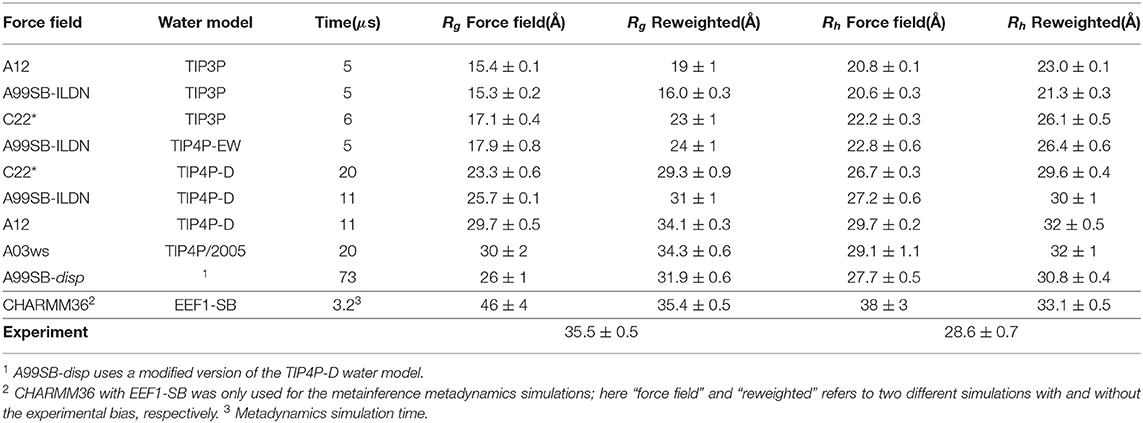
Table 1. Ensembles analyzed and refined.

We used our Bayesian/Maximum Entropy (BME) protocol (Ahmed et al., 2020; Bottaro et al., 2020) to reweight the initial force field ensembles (Table 1) with the experimental SAXS data, thus obtaining ensembles that are in closer agreement to the experimental data. Briefly described, the BME approach is based on a combined Bayesian/Maximum entropy framework, that enables one to refine a simulation using experimental data while also taking into account the potential noise in the data and in the so-called forward model used to calculate observables for the ensemble. The purpose of the reweighting is to derive a new set of weights for each configuration in a previously generated ensemble so that the reweighted ensemble satisfies the following two criteria: (i) it matches the experimental data better than the original ensemble and (ii) it achieves this improved agreement by a minimal perturbation of the original ensemble. The BME reweighting approach seeks to update the weights, w_j, by minimizing the function:

$\begin{array}{ll}{L}(w_1\dots w_n)=\frac{1}{2}{\chi }^2(w_1\dots w_n)-\theta S_{\text{rel}}(w_1\dots w_n)& (1)\end{array}$

Here, χ² quantifies the agreement between the experimental data and the corresponding observable calculated from the reweighted ensemble. $S_{rel}=-\sum _j^n{w}_j\text{log}\left(w_j/w_j^0\right)$ measures the deviation between the original ensemble weights, $w_j^0$, in our case taken as 1/n, and the reweighted ensemble weights. Finally, the hyperparameter θ tunes the balance between the two terms, and needs to be determined, by evaluating the compromise between the two terms in Equation (1) (Orioli et al., 2020). Reweighting and analysis scripts are available at github.com/KULL-Centre/papers/blob/master/2021/aSYN-ahmed-et-al/.

Metainference Metadynamics

We conducted a SAXS-restrained MD simulation using the metainference metadynamics (M&M) method, where we employed the parallel-bias (PBMetaD) flavor of well-tempered metadynamics (Pfaendtner and Bonomi, 2015) in combination with the multiple-walkers scheme (Raiteri et al., 2006). During the M&M simulation, the SAXS back-calculation step utilizes a hybrid-resolution approach, where the SAXS data is calculated on-the-fly using “Martini beads” that are superimposed on the all-atom structures using PLUMED (Bonomi and Camilloni, 2017; Paissoni et al., 2019, 2020; Jussupow et al., 2020). The approach is particularly efficient as the SAXS back-calculation is calculated using the Debye equation from a coarse-grained model and the excess of electron density in the hydration shell is neglected (Niebling et al., 2014; Paissoni et al., 2020). We note here that the Martini model is only used for calculating the SAXS data, and the simulations are performed using an all-atom, implicit solvent model as detailed below.

We used GROMACS 2018.1 (Abraham et al., 2015) with PLUMED version 2.4 (Tribello et al., 2014) to perform the M&M simulations. We used the CHARMM36 force field (Best et al., 2012) with the EEF1-SB implicit solvent model (Bottaro et al., 2013). We used a previously generated structure of αSN bound to micelles (Ulmer et al., 2005) as starting point for an initial 100-ns long high temperature (500 K) simulation, from which we extracted 64 starting conformations for the multi-replica M&M simulation. Charged amino acids were neutralized in line with the parameterization of the EEF1 model (Lazaridis and Karplus, 1999; Bottaro et al., 2013), leaving a neutral molecule, and performed a minimization to a maximum force of 100 kJ/mol/nm. The system was further equilibrated for 20 ns per replica with the metainference bias.

We performed production simulations in the NVT ensemble using Langevin dynamics (Goga et al., 2012) with a friction coefficient of 0.5 ps⁻¹ at T = 310 K, and a timestep of 2 fs. The Coulomb interactions were evaluated with a distance dependent dielectric constant of ϵ = 15r (Lazaridis and Karplus, 1999; Bottaro et al., 2013) and a cut-off at 9 Å. Constraints were applied on the hydrogens with the LINCS algorithm (Hess et al., 1997). For the production simulations the sampling of each replica was enhanced by PBMetaD along with twelve collective variables (CVs) consisting of the radius of gyration and 11 AlphaRMSD CVs to enhance sampling of local backbone conformations (Tribello et al., 2014).

Gaussians were deposited every 200 steps with a height of 0.1 kJ/mol/ps, and the σ values were set to 0.2 nm for CVrg and 0.010 for all AlphaRMSD CVs, respectively. We rescaled the height of the Gaussians using the well-tempered scheme with a bias-factor of 20 (Barducci et al., 2008).

Because calculation of the SAXS data is limiting in these simulations, we re-binned the experimental SAXS data to a set of 19 SAXS intensities at different scattering vectors, ranging between 0.01 Å⁻¹ and 0.20 Å⁻¹. Metainference was applied every 10 steps of the simulation. We used a Gaussian noise model, that applies a single Gaussian per SAXS data-point. The scaling factor between experimental and calculated SAXS intensities was sampled with a flat prior between 0.5 and 2.0 (Löhr et al., 2017). We averaged the estimated metainference weights over a time window of 200 steps; this is done to avoid large fluctuations and prevent numerical instabilities due to too high instantaneous forces (Löhr et al., 2017). The Plumed input file is available in the PLUMED-NEST database (Bonomi et al., 2019) (plumID:21.003; www.plumed-nest.org/eggs/21/003/).

Paramagnetic Relaxation Enhancement

Paramagnetic Relaxation Enhancement (PRE) via nitroxide spin-labels has been used extensively to study long-range interactions within IDPs. The measured PRE depends in particular on the distance between a paramagnetic centre and protein nuclei, in this case backbone amides. Because the PRE originates from a dipolar interaction, the observed PRE depends on r⁻⁶, and is thus particularly sensitive to transient, short distances. Because simulations were performed without the spin-labels, and because multiple spin-labels were used to probe the structural ensemble of αSN, we used a post-processing approach to estimate the location of the unpaired electron on the nitroxide label. In particular, we used DEER-PREdict (Tesei et al., 2020), which is based on a Rotamer Library Approach to place spin labels on the protein, to estimate PRE rates. We calculated and compared results from five paramagnetic labeling positions (residue: 24, 42, 62, 87, 103) in αSN (Dedmon et al., 2005). Additional details are available in the Supplementary Information and in the DEER-PREdict paper (Tesei et al., 2020).

Results and Discussion

Using αSN as an example, we compared conformational ensembles generated either directly using molecular dynamics simulations with a molecular mechanics force field, or the same ensemble refined using SAXS data. We also analyzed the results of an approach (M&M) that performs this refinement during the simulation. We thus performed (i) a SAXS-restrained multi-replica simulations using metainference metadynamics and (ii) a reference simulation both using CHARMM36 force field (Best et al., 2012) used with the EEF1-SB implicit solvent model (Bottaro et al., 2013). Both simulations consisted of 64 replicas, with one simulation using metainference to enforce the agreement with experimental SAXS data, whereas a second, reference simulation did not use experimental restraints and thus sampled the force field only. We also analyzed nine previously published multi-μs MD simulations which had been generated using different combinations of proteins force fields and water models (Piana et al., 2015; Robustelli et al., 2018) from the AMBER (Hornak et al., 2006; Best and Hummer, 2009; Lindorff-Larsen et al., 2010; Robustelli et al., 2018) and CHARMM (Piana et al., 2011) families in combination with either standard TIP3P (Jorgensen, 1981), TIP4P-EW (Horn et al., 2004), TIP4P/2005 (Abascal and Vega, 2005), or the TIP4P-D (Piana et al., 2015) water model. Table 1 summarizes the simulations and below we refer to the prior (not refined) ensemble as the “force field” ensemble and the posterior (refined) ensemble as the “reweighted” ensemble.

Force Field Accuracy and Sampling

Before the refinement procedure we calculated SAXS intensity curves from each structure in the ensembles using PEPSI-SAXS (Grudinin et al., 2017). We also calculated the R_g from the protein coordinates and used them to estimate the hydrodynamic radius (R_h) for each conformation using a previously described empirical relationship (Nygaard et al., 2017; Ahmed et al., 2020) (Table 1). The experimental R_g = 35.5 Å was obtained through Guinier analysis of the experimental SAXS curve (see Methods), while the experimental R_h = 29.0 Å was obtained through NMR diffusion measurements (Table 1).

In line with previous observations (Piana et al., 2015; Robustelli et al., 2018), the ensembles show very different levels of compaction depending on the force field and, in particular, water model used (Table 1 and Figure 1). When paired with the TIP3P water model, both the Amber or CHARMM force fields produce very compact conformations and show poor agreement with the experimental value of R_g. On the other hand, when paired with the recently parameterized TIP4P-D water model the force fields give rise to more expanded structures and match the experimental values of R_g and R_h considerably better. The ensemble generated using CHARMM36 with the EEF1-SB implicit solvent model on the other-hand produce more expanded structures (Table 1). Of particular relevance to the reweighting described below it is worth noting how the compact ensembles either do not sample any, or at most very few, structures that are expanded as the average R_g observed in experiment (Figure 1). This observation already suggests that it will be difficult robustly to derive ensembles that are in agreement with the SAXS data as this in particular is sensitive to the R_g.

FIGURE 1

Figure 1. Radius of gyration during simulations with different force fields and water models. As representative examples we show the time-evolution of the radius of gyration for simulations of αSN performed with the A12 force field (orange), C22* (blue), and A12 (green) with the TIP4P-D, TIP4P-D, and TIP3P water model, respectively. The experimental value (black) was obtained from a Guinier analysis of the SAXS data. The orange and blue curves have been smoothed to ease visualization. The insert shows probability densities and averages of R_g. Representative structures with different degrees of compaction are also shown. The length of the simulations is 11, 20, and 5 μs, respectively, but are shown here on a normalized timescale to make comparisons easier.

Ensemble Refinement Using SAXS Data

In the following section we exemplify the BME refinement against the SAXS data using two representative combinations of force field and water models, specifically A12 paired with either the TIP3P or the TIP4P-D water model (Figure 2). We also present the results obtained from “on-the-fly” SAXS-restrained simulation with M&M which we compared to an unrestrained simulation with otherwise identical simulation settings (see Methods). Note that while the R_g values for the simulations were calculated using protein coordinates, the experimental value also includes potential contributions from the solvent. The refinement, analysis and plots for the remaining force fields are shown in the supplementary information (Supplementary Figures 4–10).

FIGURE 2

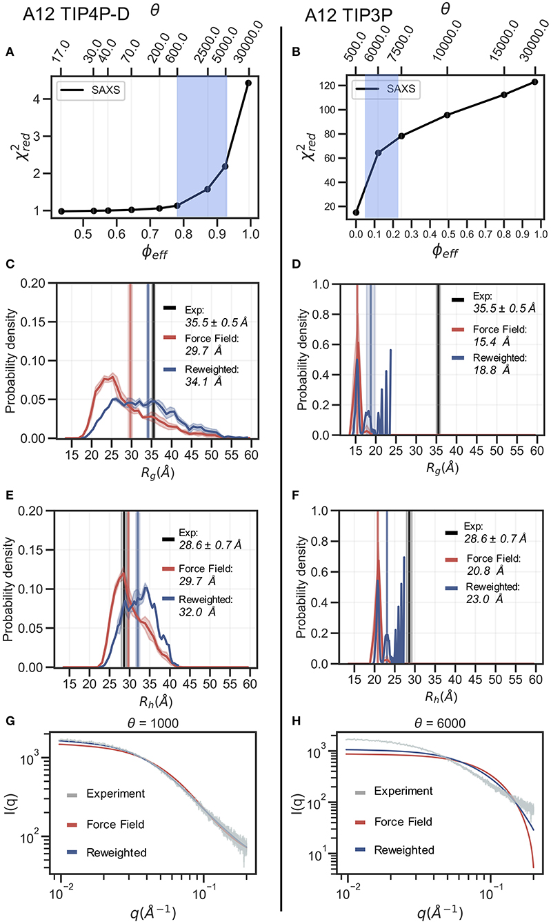
Figure 2. Refinement of two ensembles using BME with SAXS data. SAXS refinement of an ensemble sampled with A12 and either (left) the TIP4P-D water model or (right) the TIP3P water model. (A,B) In the L-curve analysis to select the parameter θ we plot χ² against ϕ_eff. θ balances the prior (force field) and the experimental data, ϕ_eff is the effective number of frames used in the final reweighted ensemble. A value of θ is selected from the region marked in blue. We here used θ = 1,000 and θ = 6,000 for the TIP4P-D ensemble and TIP3P ensemble, respectively. Probability distribution of (C,D) R_g and (E,F) R_h for the prior (red) and reweighted (blue) ensembles. Solid vertical lines represent the ensemble averaged R_g and R_h. The experimental values are shown in black. The error of the distributions and on the averages (shown as shades) were estimated by block averaging. (G,H) Calculated SAXS intensities from the prior ensemble and the reweighted ensembles are compared to the experimental SAXS data.

The BME procedure works by assigning weights to a previously generated ensemble so as to fit the experimental data better. For BME to successfully reweight an ensemble it is thus required that the initial prior ensemble contains the most relevant conformational states of the protein, such that the ensemble that gives rise to the experimental data is a sub-ensemble of the initial prior ensemble. Consequently, if the sampling is incomplete or the unbiased ensemble is very far away from the true ensemble, it may not be possible to reweight the ensemble to reach a satisfactory agreement with the experiments. An indication that this is occurring is that BME will effectively down-weight most of the structures in the prior ensemble and the posterior ensemble will be dominated by a few structures with large weights. This can in turn be quantified by calculating the (effective) fraction of structures, ϕ_eff = exp(S_rel), that contribute to the ensemble (Orioli et al., 2020), so that when ϕ_eff ≈ 1 most of the structures are retained, whereas ϕ_eff ≈ 0 indicates a few structures with very large weights

In the BME reweighting the confidence in the prior ensemble with respect to the experimental data can be tuned by the hyper-parameter θ (Equation 1). One usually does not know the optimal value for θ beforehand. Here, we choose θ by performing an L-curve analysis (Hansen and O'Leary, 1993; Orioli et al., 2020) in which we plot the ${\chi }_{red}^2$ value (quantifying the difference between experiments and calculated value) as a function of ϕ_eff, for different values of θ and choose a value corresponding to the “elbow” region (blue region in Figures 2A,B). The L-curve analysis for the A12 force field paired with TIP4P-D water model, lead us to choose θ = 1, 000, after which the ensemble retains 88% of the initial structures in the final reweighted ensemble, and show much better agreement with the experimental data, indicative by a low ${\chi }_{red}^2$ (Figure 2A). In contrast, the analysis for the TIP3P water model, after reweighting with θ = 6, 000, show that only 12% of the initial structures are used in the final reweighted ensemble in order to achieve significant improved agreement with the experimental data (Figure 2B). Even at a lower θ value there is still a large discrepancy between experimental and calculated SAXS data (${\chi }_{red}^2=17$ at θ = 500). This is a clear example of a poor prior ensemble, which is caused by insufficient overlap between the force field ensemble and that probed by experiment. In fact, the highest value observed (R_g =23 Å) is significantly lower than the experimental value (black). As a consequence, BME ‘throws out’ most of the structures from the initial force field ensemble, and the final reweighted ensemble mainly consist of a few highly weighted structures (Figure 2D).

The ensemble generated with the TIP4P-D water model (Figure 2C) contains structures that span a greater range of R_g values, both above and below the experimental value. After refinement, the reweighted ensemble is shifted to give greater weight to more expanded structures and bringing the average R_g substantially closer to the value estimated from the SAXS data. We note here that we do not fit the R_g value but rather the SAXS data. Because the experimental value of R_g (obtained from a Guinier analyses of the data) contains a contribution from the solvent we do not expect a perfect agreement with the average R_g calculated from the protein coordinates (Henriques et al., 2018). Indeed, this is one of the reasons why we fit the SAXS data directly rather than the R_g.

The effect of reweighting of the two ensembles can also be seen on the distributions of R_h (Figures 2E,F). Similar to R_g distributions, the TIP4P-D ensemble is shifted to give greater weight to more expanded structures (Figure 2E). As was also evident from the distribution of R_g, the more compact TIP3P ensemble gives rise to a very noisy distribution, because the reweighted ensemble predominantly consists of a few highly weighted structures (Figure 2F). To illustrate the consequences of reweighting we also compared the calculated SAXS data from the initial force field and reweighted ensembles to the experimental scattering data (Figures 2G,H). As expected, the refined ensembles show better agreement with experiments, in particular for the A12 paired with TIP4P-D. As agreement between experimental and calculated data is the target for BME this observation again just illustrates that the BME method is indeed optimizing agreement.

We repeated these analyses for the remaining combinations of force fields and water models (Supplementary Figures 4–10) and summarize the results by assessing how well the ensembles reproduce R_g and R_h before and after refinement (Figure 3). We note that the improvement of the R_g observed is due to the use of SAXS data in the refinement, as SAXS intensity curve inherently contains information of the R_g, and that improved agreement with the R_g is thus a sign of the BME approach working rather than a validation of the ensemble.

FIGURE 3

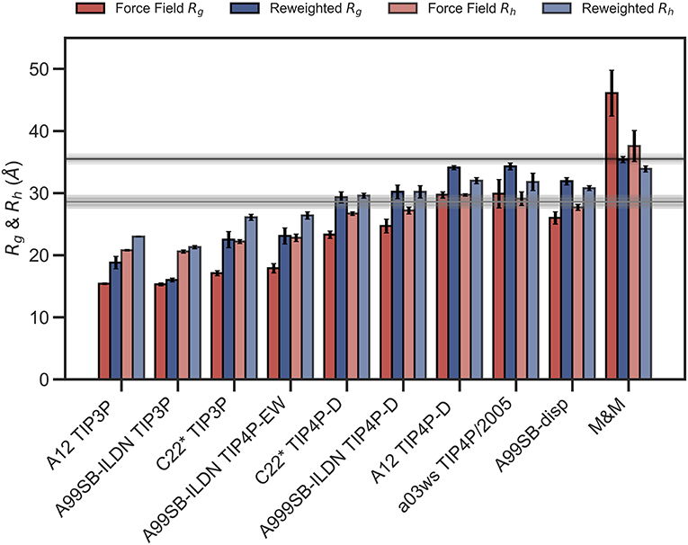
Figure 3. Radius of gyration and hydrodynamic radius calculated from the initial force field ensemble (red) and the experimentally refined ensembles (blue). Experimental values from SAXS (R_g = 35.5Å) and NMR (R_h = 29.0Å) are shown as horizontal lines with the shaded area indicating the error of the experimental values.

To evaluate the effectiveness of the SAXS-restrained M&M simulation we monitored the agreement between the back-calculated and the experimental data over the simulation time by monitoring their correlation rather than the χ² (Paissoni et al., 2020). Both the SAXS-restrained and the unrestrained reference simulation show a high correlation between back-calculated and experimental data (>0.98) (Supplementary Figure 3A). As expected, the agreement improves substantially when the experimental data is used as a bias in the metainference simulations, confirming the effectiveness of the inclusion of experimental SAXS data (Supplementary Figure 3A). Likewise, the average R_g, R_h and the back-calculated SAXS intensity data show improved agreement with the experimental data in the metainference produced ensemble (Figure 3 and Supplementary Figure 3).

In total our analyses show that it is possible to refine MD simulations against SAXS data, though the extent to which agreement can be reached depends on the quality of the input ensemble. For the most compact ensembles we are able to increase the average compaction by fitting to the data, though the average R_g and R_h are still substantially below the experimental values. While the SAXS data (and thus R_g) were used as target values, we also cross-validated with R_h which was not used in the fitting. Here, the picture is less clear. Overall, for the more compact ensembles, fitting the SAXS data lead to improved prediction of R_h. For other ensembles, such as A12 with TIP4P-D, that show good agreement with R_h before reweighting, the agreement became slightly worse after reweighting. Finally, for the most expanded ensemble obtained with CHARMM36/EEF1-SB, agreement with R_h improved after biasing with the SAXS data. As discussed further below, the approach that we use to estimate R_h from the ensembles is approximate and requires further assessment before these small differences can be interpreted in detail.

Validation With PRE Data

PRE experiments probe the population-weighted average of the distance (as r⁻⁶) between a paramagnetic centre and protein nuclei and, given the r⁻⁶ dependency, is sensitive to the shorter distances even if the populations are small. Here, we compare previously published PREs from spin-labeled αSN (Dedmon et al., 2005) and back-calculated PRE intensity ratios from five labeling sites, for each of the force fields in Table 1, before and after refinement (see also Supporting Information). PRE intensity-ratio profiles from a more expanded ensemble generated using A12 with TIP4P-D (Figure 4A) and a more compact one generated with A12 with TIP3P (Figure 4B) show clear differences in agreement with experiments before refinement with the SAXS data.

FIGURE 4

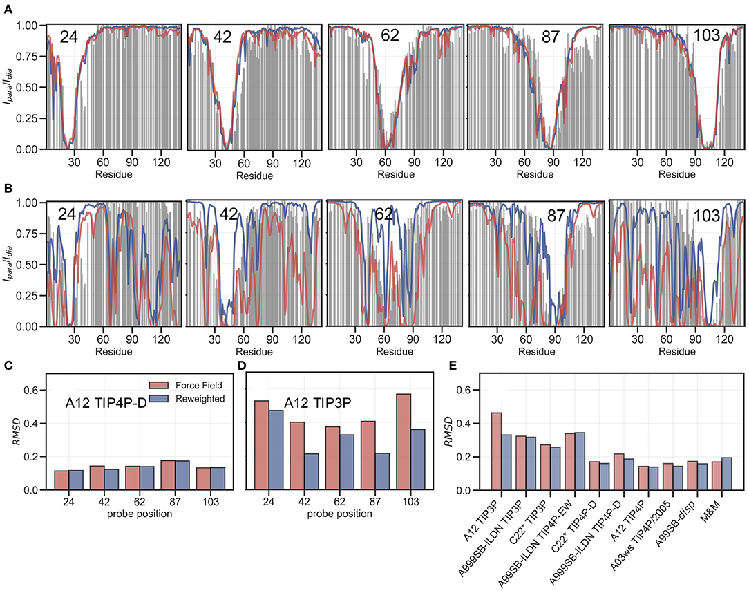
Figure 4. Comparing ensembles to PRE data. We calculated the PRE intensity ratios both from the prior (red) and the reweighted (blue) ensembles and compared to the experimental data (gray). As representative examples we again show results with the A12 protein force field combined with either (A) TIP4P-D or (B) TIP3P water models, and where the location of the spin label probe is denoted in each plot. Experimental intensity ratios slightly exceeding the value 1 were set to 1 in these plots. (C,D) We also calculated the RMSD between the experimental and calculated intensity ratios for each probe and the two force fields both before and after reweighting. (E) Finally, we calculated the RMSD between experiment and calculated values over all probe position for and all force fields in Table 1.

BME refinement leads only to small changes in the calculated PRE data for A12/TIP4P-D, whereas the selection of more expanded structures, by applying BME to the ensemble generated with A12/TIP3P, leads to more substantial changes as quantified for example by calculating the RMSD between simulation and experimental data (Figures 4C,D). We performed similar calculations and analyses for all ensembles (Supplementary Figures 11–18) and summarize the overall RMSD before and after BME (Figure 4E). For the force fields paired with TIP3P in particular, we observe many of the long-range contacts diminish after reweighting. These results suggest that the reweighting decreases contributions from structures that are too compact, and that the final reweighted ensemble contains more extended structures. In the TIP4P-D ensembles we still observe that some long-range contacts persist even after reweighting and the better agreement is not alone achieved at the cost of a complete elimination of long-range contacts; nevertheless, the improvements of the PREs are generally small for these ensembles, and in the case of the metainference ensemble we even observe a small worsening of the agreement.

Comparison of Ensembles

An important question is whether and how much ensembles become more similar to one another after reweighting using experimental data. Clearly, the properties of the final ensembles reflect information both in the prior and in the experimental data. Previously we and others have shown that experimental data make ensembles more similar to one another (Lindorff-Larsen and Ferkinghoff-Borg, 2009; Camilloni et al., 2012; Tiberti et al., 2015; Larsen et al., 2020), though the extent to which this occurs depends on how the ensembles are compared.

The results described above suggest that the description of the level of compaction indeed becomes more similar after reweighting, and this is reflected also in more similar distribution of the radius of gyration (Supplementary Figure 19). Nevertheless, it is also clear that differences remain, in particular when the prior gives a very poor description of the data. A more complex situation arises when the ensembles are compared using properties that are only little correlated with those probed by the SAXS experiments, such as for example local (secondary) structure. We therefore used STRIDE (Frishman and Argos, 1995) to calculate the secondary structure in all ensembles, both before and after reweighting with the SAXS data (Supplementary Figures 19, 20). As also previously shown (Robustelli et al., 2018) there is little transient helical structure in these simulations, though with some variation across force fields. Previous analyses suggest that compaction and secondary structure are only weakly coupled in disordered proteins (Piana et al., 2012; Crehuet et al., 2019; Zerze et al., 2019), and indeed we in general find that reweighting against the SAXS data only has a modest effect on the secondary structure. The M&M simulations, however, do not follow this pattern, but we note here that in contrast to the other simulations, these are two independent simulations. In summary, these analyses demonstrate that inclusion of experimental restraints make ensembles more similar in some properties, but not necessarily in others. Reweighting against a set of experimental data will thus only affect properties that affect, or are otherwise coupled to, the experimental data. As argued previously (Crehuet et al., 2019), this also means that cross-validation is only useful when using types of experiments that probe related molecular properties.

Conclusions

We have employed “on-the-fly” or “post-facto” integration of MD simulations and SAXS data αSN to derive structural ensembles that are in improved agreement with experiments. These approaches take their outset in a Bayesian framework, and thus the results of the posterior distribution may depend on the choice of the prior. Our results clearly show, in line with previous observations (Larsen et al., 2020), that if the prior distribution is a poor model for the experimental data, reweighting becomes noisy. Despite this we find that fitting against SAXS data generally improved or had no effect on the agreement with NMR data (R_h and PREs) that were not target of the optimization. Thus, the inclusion of a SAXS-restraint in the metainference simulation and the BME refinement showed that both methods were able to generate a reliable and heterogenous ensemble that maintained good agreement with independent experimental data. We nevertheless also find that the prior used in such protocols are important, and that more robust analyses are obtained with the best priors.

Our results also reflect an important point when including experimental data to refine ensembles, namely that the ensembles will only be affected along degrees of freedom that are sensitive to the experiments (or vice versa). Thus, as shown by our analyses, while the level of compaction (p(R_g)) becomes more similar after inclusion of the SAXS data, this is not the case for the description of the secondary structure. In order to improve the description of both global and local structure one thus needs to include data sensitive to both properties, either individually (such as SAXS and chemical shifts) or combined such as residual dipolar couplings.

Our calculations of R_h and PREs suggest that when the ensembles are “far” away from the experimental data, then improvements driven by the SAXS refinement lead to clear improvements in independent parameters. For ensembles that show better agreement between with the SAXS data to begin with, the picture is less clear. While we on average observe improvements, they are often modest. While some of this is likely because the ensembles are already in reasonably good agreement with the experiment, we also suggest that we are observing the limitations of the forward models for calculating SAXS, R_h and PREs. In particular, we suggest that more research is needed on comparing the accuracy and domains of applicability of existing methods for calculating R_h (Kirkwood and Riseman, 1948; de la Torre et al., 2000; Nygaard et al., 2017; Fleming and Fleming, 2018). Methods for calculating SAXS data (Henriques et al., 2018; Hub, 2018), however, also require choices to be made for how to deal with solvent effects, and calculations of PREs rely on models and parameters to describe effects of dynamics (Tesei et al., 2020). In all cases, further work is needed to make it possible to extract as much as possible information from the data, such as for example the independent information about the moments of the R_g-distribution contained within the SAXS and NMR diffusion measurements (Choy et al., 2002; Ahmed et al., 2020).

Thus, we conclude that in order to obtain improved descriptions of the conformational ensembles of disordered proteins, work is needed in several areas. First, improved force fields and sampling methods give rise to better initial estimates that require less (or no) reweighting. Second, refinement should ideally use data from experiments that are sensitive to as many conformational properties as possible, and at least those that probe the properties of interest. Finally, improved and consistent forward models are required to use this data to provide better models for intrinsically disordered proteins. Importantly, these different aspects work in synergy as accurate prior ensembles are more robust toward reweighting, and that accurate forward models make it possible to extract more information from the experimental data.

Data Availability Statement

The datasets presented in this study can be found in online repositories. The names of the repository/repositories and accession number(s) can be found at: https://github.com/KULL-Centre/papers/blob/master/2021/aSYN-ahmed-et-al/, https://www.plumed-nest.org/eggs/21/003/.

Author Contributions

MCA analyzed and performed MD simulations, analyzed the data, wrote the first draft, and made figures. LKS purified αSN, and performed and analyzed SAXS data together with AEL. AJ and CC developed the simulation procedure with MCA, and aided in metainference simulations. EAN purified αSN, and performed and analyzed NMR data together with BBK. KL-L designed the research, supervised MCA, analyzed the data, and revised the article. All authors contributed to the article and approved the submitted version.

Funding

We acknowledge support by a grant from the Lundbeck Foundation to the BRAINSTRUC Structural Biology Initiative (R155-2015-2666). The funders had no role in study design, data collection and analysis, decision to publish, or preparation of the manuscript.

Conflict of Interest

The authors declare that the research was conducted in the absence of any commercial or financial relationships that could be construed as a potential conflict of interest.

Acknowledgments

We thank A. Kikhney and C. Jeffries for assistance during data collection at the P12 SAXS beamline. We thank D. E. Shaw Research for sharing the molecular dynamics trajectories.

Supplementary Material

The Supplementary Material for this article can be found online at: https://www.frontiersin.org/articles/10.3389/fmolb.2021.654333/full#supplementary-material

References

Abascal, J. L., and Vega, C. (2005). A general purpose model for the condensed phases of water: Tip4p/2005. J. Chem. Phys. 123:234505. doi: 10.1063/1.2121687

PubMed Abstract | CrossRef Full Text | Google Scholar

Abraham, M. J., Murtola, T., Schulz, R., Páll, S., Smith, J. C., Hess, B., et al. (2015). Gromacs: high performance molecular simulations through multi-level parallelism from laptops to supercomputers. SoftwareX 1, 19–25. doi: 10.1016/j.softx.2015.06.001

CrossRef Full Text | Google Scholar

Ahmed, M. C., Crehuet, R., and Lindorff-Larsen, K. (2020). Computing, analyzing, and comparing the radius of gyration and hydrodynamic radius in conformational ensembles of intrinsically disordered proteins. Methods Mol. Biol. 2141, 429–445. doi: 10.1007/978-1-0716-0524-0_21

PubMed Abstract | CrossRef Full Text | Google Scholar

Barducci, A., Bussi, G., and Parrinello, M. (2008). Well-tempered metadynamics: a smoothly converging and tunable free-energy method. Phys. Rev. Lett. 100:020603. doi: 10.1103/PhysRevLett.100.020603

PubMed Abstract | CrossRef Full Text | Google Scholar

Bernado, P., and Svergun, D. I. (2012). Structural analysis of intrinsically disordered proteins by small-angle X-ray scattering. Mol. Biosyst. 8, 151–167. doi: 10.1039/C1MB05275F

PubMed Abstract | CrossRef Full Text | Google Scholar

Best, R. B., and Hummer, G. (2009). Optimized molecular dynamics force fields applied to the helix-coil transition of polypeptides. J. Phys. Chem. B 113, 9004–9015. doi: 10.1021/jp901540t

PubMed Abstract | CrossRef Full Text | Google Scholar

Best, R. B., Zheng, W., and Mittal, J. (2014). Balanced protein-water interactions improve properties of disordered proteins and non-specific protein association. J. Chem. Theory Comput. 10, 5113–5124. doi: 10.1021/ct500569b

PubMed Abstract | CrossRef Full Text | Google Scholar

Best, R. B., Zhu, X., Shim, J., Lopes, P. E., Mittal, J., Feig, M., et al. (2012). Optimization of the additive charmm all-atom protein force field targeting improved sampling of the backbone ϕ, ψ and side-chain χ1 and χ2 dihedral angles. J. Chem. Theory Comput. 8, 3257–3273. doi: 10.1021/ct300400x

CrossRef Full Text | Google Scholar

Blanchet, C. E., Spilotros, A., Schwemmer, F., Graewert, M. A., Kikhney, A., Jeffries, C. M., et al. (2015). Versatile sample environments and automation for biological solution X-ray scattering experiments at the P12 beamline (PETRA III, DESY). J. Appl. Crystallogr. 48, 431–443. doi: 10.1107/S160057671500254X

PubMed Abstract | CrossRef Full Text | Google Scholar

Bonomi, M., Bussi, G., Camilloni, C., and Tribello, G. A. (2019). Promoting transparency and reproducibility in enhanced molecular simulations. Nat. Methods 16, 670–673. doi: 10.1038/s41592-019-0506-8

PubMed Abstract | CrossRef Full Text | Google Scholar

Bonomi, M., and Camilloni, C. (2017). Integrative structural and dynamical biology with PLUMED-ISDB. Bioinformatics 33, 3999–4000. doi: 10.1093/bioinformatics/btx529

PubMed Abstract | CrossRef Full Text | Google Scholar

Bonomi, M., Camilloni, C., Cavalli, A., and Vendruscolo, M. (2016a). Metainference: a bayesian inference method for heterogeneous systems. Sci. Adv. 2:e1501177. doi: 10.1126/sciadv.1501177

PubMed Abstract | CrossRef Full Text | Google Scholar

Bonomi, M., Camilloni, C., and Vendruscolo, M. (2016b). Metadynamic metainference: enhanced sampling of the metainference ensemble using metadynamics. Sci. Rep. 6:31232. doi: 10.1038/srep31232

PubMed Abstract | CrossRef Full Text | Google Scholar

Bottaro, S., Bengtsen, T., and Lindorff-Larsen, K. (2020). Integrating molecular simulation and experimental data: a bayesian/maximum entropy reweighting approach. Methods Mol. Biol. 2112, 219–240. doi: 10.1007/978-1-0716-0270-6_15

PubMed Abstract | CrossRef Full Text | Google Scholar

Bottaro, S., Lindorff-Larsen, K., and Best, R. B. (2013). Variational optimization of an all-atom implicit solvent force field to match explicit solvent simulation data. J. Chem. Theory Comput. 9, 5641–5652. doi: 10.1021/ct400730n

PubMed Abstract | CrossRef Full Text | Google Scholar

Box, G. E., and Tiao, G. C. (2011). Bayesian Inference in Statistical Analysis, Vol. 40. Hoboken, NJ: John Wiley & Sons.

Google Scholar

Camilloni, C., Robustelli, P., Simone, A. D., Cavalli, A., and Vendruscolo, M. (2012). Characterization of the conformational equilibrium between the two major substates of rnase a using NMR chemical shifts. J. Am. Chem. Soc. 134, 3968–3971. doi: 10.1021/ja210951z

PubMed Abstract | CrossRef Full Text | Google Scholar

Cesari, A., Reißer, S., and Bussi, G. (2018). Using the maximum entropy principle to combine simulations and solution experiments. Computation 6:15. doi: 10.3390/computation6010015

PubMed Abstract | CrossRef Full Text | Google Scholar

Chemes, L. B., Alonso, L. G., Noval, M. G., and de Prat-Gay, G. (2012). Circular dichroism techniques for the analysis of intrinsically disordered proteins and domains. Methods Mol. Biol. 895, 387–404. doi: 10.1007/978-1-61779-927-3_22

PubMed Abstract | CrossRef Full Text | Google Scholar

Choy, W.-Y., Mulder, F. A., Crowhurst, K. A., Muhandiram, D., Millett, I. S., Doniach, S., et al. (2002). Distribution of molecular size within an unfolded state ensemble using small-angle X-ray scattering and pulse field gradient NMR techniques. J. Mol. Biol. 316, 101–112. doi: 10.1006/jmbi.2001.5328

PubMed Abstract | CrossRef Full Text | Google Scholar

Crehuet, R., Buigues, P. J., Salvatella, X., and Lindorff-Larsen, K. (2019). Bayesian-maximum-entropy reweighting of IDP ensembles based on NMR chemical shifts. Entropy 21:898. doi: 10.3390/e21090898

CrossRef Full Text | Google Scholar

Das, R. K., Ruff, K. M., and Pappu, R. V. (2015). Relating sequence encoded information to form and function of intrinsically disordered proteins. Curr. Opin. Struct. Biol. 32, 102–112. doi: 10.1016/j.sbi.2015.03.008

PubMed Abstract | CrossRef Full Text | Google Scholar

de la Torre, J. G., Huertas, M. L., and Carrasco, B. (2000). Calculation of hydrodynamic properties of globular proteins from their atomic-level structure. Biophys. J. 78, 719–730. doi: 10.1016/S0006-3495(00)76630-6

PubMed Abstract | CrossRef Full Text | Google Scholar

Dedmon, M. M., Lindorff-Larsen, K., Christodoulou, J., Vendruscolo, M., and Dobson, C. M. (2005). Mapping long-range interactions in α-synuclein using spin-label NMR and ensemble molecular dynamics simulations. J. Am. Chem. Soc. 127, 476–477. doi: 10.1021/ja044834j

PubMed Abstract | CrossRef Full Text | Google Scholar

Dyson, H. J., and Wright, P. E. (2001). Nuclear magnetic resonance methods for elucidation of structure and dynamics in disordered states. Methods Enzymol. 339, 258–270. doi: 10.1016/S0076-6879(01)39317-5

PubMed Abstract | CrossRef Full Text | Google Scholar

Eliezer, D. (2009). Biophysical characterization of intrinsically disordered proteins. Curr. Opin. Struct. Biol. 19, 23–30. doi: 10.1016/j.sbi.2008.12.004

PubMed Abstract | CrossRef Full Text | Google Scholar

Fleming, P. J., and Fleming, K. G. (2018). Hullrad: fast calculations of folded and disordered protein and nucleic acid hydrodynamic properties. Biophys. J. 114, 856–869. doi: 10.1016/j.bpj.2018.01.002

PubMed Abstract | CrossRef Full Text | Google Scholar

Frishman, D., and Argos, P. (1995). Knowledge-based protein secondary structure assignment. Proteins 23, 566–579. doi: 10.1002/prot.340230412

PubMed Abstract | CrossRef Full Text | Google Scholar

Goga, N., Rzepiela, A., De Vries, A., Marrink, S., and Berendsen, H. (2012). Efficient algorithms for Langevin and DPD dynamics. J. Chem. Theory Comput. 8, 3637–3649. doi: 10.1021/ct3000876

PubMed Abstract | CrossRef Full Text | Google Scholar

Grudinin, S., Garkavenko, M., and Kazennov, A. (2017). PEPSI-SAXS: an adaptive method for rapid and accurate computation of small-angle X-ray scattering profiles. Acta Crystallogr. D 73, 449–464. doi: 10.1107/S2059798317005745

PubMed Abstract | CrossRef Full Text | Google Scholar

Hansen, P. C., and O'Leary, D. P. (1993). The use of the L-curve in the regularization of discrete ill-posed problems. SIAM J. Sci. Comput. 14, 1487–1503. doi: 10.1137/0914086

CrossRef Full Text | Google Scholar

Henriques, J., Arleth, L., Lindorff-Larsen, K., and Skepö, M. (2018). On the calculation of SAXS profiles of folded and intrinsically disordered proteins from computer simulations. J. Mol. Biol. 430, 2521–2539. doi: 10.1016/j.jmb.2018.03.002

PubMed Abstract | CrossRef Full Text | Google Scholar

Hermann, M. R., and Hub, J. S. (2019). SAXS-restrained ensemble simulations of intrinsically disordered proteins with commitment to the principle of maximum entropy. J. Chem. Theory Comput. 15, 5103–5115. doi: 10.1021/acs.jctc.9b00338

PubMed Abstract | CrossRef Full Text | Google Scholar

Hess, B., Bekker, H., Berendsen, H. J., and Fraaije, J. G. (1997). Lincs: a linear constraint solver for molecular simulations. J. Comput. Chem. 18, 1463–1472. doi: 10.1002/(SICI)1096-987X(199709)18:12<1463::AID-JCC4>3.0.CO;2-H

CrossRef Full Text | Google Scholar

Horn, H. W., Swope, W. C., Pitera, J. W., Madura, J. D., Dick, T. J., Hura, G. L., et al. (2004). Development of an improved four-site water model for biomolecular simulations: Tip4p-ew. J. Chem. Phys. 120, 9665–9678. doi: 10.1063/1.1683075

PubMed Abstract | CrossRef Full Text | Google Scholar

Hornak, V., Abel, R., Okur, A., Strockbine, B., Roitberg, A., and Simmerling, C. (2006). Comparison of multiple amber force fields and development of improved protein backbone parameters. Proteins 65, 712–725. doi: 10.1002/prot.21123

PubMed Abstract | CrossRef Full Text | Google Scholar

Hub, J. S. (2018). Interpreting solution X-ray scattering data using molecular simulations. Curr. Opin. Struct. Biol. 49, 18–26. doi: 10.1016/j.sbi.2017.11.002

PubMed Abstract | CrossRef Full Text | Google Scholar

Hummer, G., and Köfinger, J. (2015). Bayesian ensemble refinement by replica simulations and reweighting. J. Chem. Phys. 143, 12B634_1. doi: 10.1063/1.4937786

PubMed Abstract | CrossRef Full Text | Google Scholar

Jaynes, E. T. (1957). Information theory and statistical mechanics. Phys. Rev. 106:620. doi: 10.1103/PhysRev.106.620

CrossRef Full Text | Google Scholar

Jorgensen, W. L. (1981). Quantum and statistical mechanical studies of liquids. 10. Transferable intermolecular potential functions for water, alcohols, and ethers. application to liquid water. J. Am. Chem. Soc. 103, 335–340. doi: 10.1021/ja00392a016

CrossRef Full Text | Google Scholar

Jussupow, A., Messias, A. C., Stehle, R., Geerlof, A., Solbak, S. M., Paissoni, C., et al. (2020). The dynamics of linear polyubiquitin. Sci. Adv. 6:eabc3786. doi: 10.1126/sciadv.abc3786

CrossRef Full Text | Google Scholar

Kirkwood, J. G., and Riseman, J. (1948). The intrinsic viscosities and diffusion constants of flexible macromolecules in solution. J. Chem. Phys. 16, 565–573. doi: 10.1063/1.1746947

CrossRef Full Text | Google Scholar

Laio, A., and Parrinello, M. (2002). Escaping free-energy minima. Proc. Natl. Acad. Sci. U.S.A. 99, 12562–12566. doi: 10.1073/pnas.202427399

CrossRef Full Text | Google Scholar

Larsen, A. H., Wang, Y., Bottaro, S., Grudinin, S., Arleth, L., and Lindorff-Larsen, K. (2020). Combining molecular dynamics simulations with small-angle X-ray and neutron scattering data to study multi-domain proteins in solution. PLoS Comput. Biol. 16:e1007870. doi: 10.1371/journal.pcbi.1007870

PubMed Abstract | CrossRef Full Text | Google Scholar

Lazaridis, T., and Karplus, M. (1999). Effective energy function for proteins in solution. Proteins 35, 133–152. doi: 10.1002/(SICI)1097-0134(19990501)35:2<133::AID-PROT1>3.0.CO;2-N

PubMed Abstract | CrossRef Full Text | Google Scholar

LeBlanc, S., Kulkarni, P., and Weninger, K. (2018). Single molecule FRET: a powerful tool to study intrinsically disordered proteins. Biomolecules 8:140. doi: 10.3390/biom8040140

PubMed Abstract | CrossRef Full Text | Google Scholar

Lindorff-Larsen, K., and Ferkinghoff-Borg, J. (2009). Similarity measures for protein ensembles. PLoS ONE 4:e4203. doi: 10.1371/journal.pone.0004203

CrossRef Full Text | Google Scholar

Lindorff-Larsen, K., Piana, S., Palmo, K., Maragakis, P., Klepeis, J. L., Dror, R. O., et al. (2010). Improved side-chain torsion potentials for the amber FF99SB protein force field. Proteins 78, 1950–1958. doi: 10.1002/prot.22711

PubMed Abstract | CrossRef Full Text | Google Scholar

Löhr, T., Jussupow, A., and Camilloni, C. (2017). Metadynamic metainference: convergence towards force field independent structural ensembles of a disordered peptide. J. Chem. Phys. 146:165102. doi: 10.1063/1.4981211

PubMed Abstract | CrossRef Full Text | Google Scholar

Nerenberg, P. S., Jo, B., So, C., Tripathy, A., and Head-Gordon, T. (2012). Optimizing solute-water van der Waals interactions to reproduce solvation free energies. J. Phys. Chem. B 116, 4524–4534. doi: 10.1021/jp2118373

PubMed Abstract | CrossRef Full Text | Google Scholar

Niebling, S., Björling, A., and Westenhoff, S. (2014). Martini bead form factors for the analysis of time-resolved X-ray scattering of proteins. J. Appl. Crystallogr. 47, 1190–1198. doi: 10.1107/S1600576714009959

PubMed Abstract | CrossRef Full Text | Google Scholar

Nygaard, M., Kragelund, B. B., Papaleo, E., and Lindorff-Larsen, K. (2017). An efficient method for estimating the hydrodynamic radius of disordered protein conformations. Biophys. J. 113, 550–557. doi: 10.1016/j.bpj.2017.06.042

PubMed Abstract | CrossRef Full Text | Google Scholar

Orioli, S., Larsen, A. H., Bottaro, S., and Lindorff-Larsen, K. (2020). How to learn from inconsistencies: integrating molecular simulations with experimental data. Prog. Mol. Biol. Transl. Sci. 170, 123–176. doi: 10.1016/bs.pmbts.2019.12.006

PubMed Abstract | CrossRef Full Text | Google Scholar

Paissoni, C., Jussupow, A., and Camilloni, C. (2019). Martini bead form factors for nucleic acids and their application in the refinement of protein-nucleic acid complexes against SAXS data. J. Appl. Crystallogr. 52, 394–402. doi: 10.1107/S1600576719002450

CrossRef Full Text | Google Scholar

Paissoni, C., Jussupow, A., and Camilloni, C. (2020). Determination of protein structural ensembles by hybrid-resolution SAXS restrained molecular dynamics. J. Chem. Theory Comput. 16, 2825–2834. doi: 10.1021/acs.jctc.9b01181

PubMed Abstract | CrossRef Full Text | Google Scholar

Panjkovich, A., and Svergun, D. I. (2018). Chromixs: automatic and interactive analysis of chromatography-coupled small angle X-ray scattering data. Bioinformatics 34, 1944–1946. doi: 10.1093/bioinformatics/btx846

PubMed Abstract | CrossRef Full Text | Google Scholar

Pfaendtner, J., and Bonomi, M. (2015). Efficient sampling of high-dimensional free-energy landscapes with parallel bias metadynamics. J. Chem. Theory Comput. 11, 5062–5067. doi: 10.1021/acs.jctc.5b00846

PubMed Abstract | CrossRef Full Text | Google Scholar

Piana, S., Donchev, A. G., Robustelli, P., and Shaw, D. E. (2015). Water dispersion interactions strongly influence simulated structural properties of disordered protein states. J. Phys. Chem. B 119, 5113–5123. doi: 10.1021/jp508971m

PubMed Abstract | CrossRef Full Text | Google Scholar

Piana, S., Lindorff-Larsen, K., Dirks, R. M., Salmon, J. K., Dror, R. O., and Shaw, D. E. (2012). Evaluating the effects of cutoffs and treatment of long-range electrostatics in protein folding simulations. PLoS ONE 7:e39918. doi: 10.1371/journal.pone.0039918

PubMed Abstract | CrossRef Full Text | Google Scholar

Piana, S., Lindorff-Larsen, K., and Shaw, D. E. (2011). How robust are protein folding simulations with respect to force field parameterization? Biophys. J. 100, L47–L49. doi: 10.1016/j.bpj.2011.03.051

PubMed Abstract | CrossRef Full Text | Google Scholar

Prestel, A., Bugge, K., Staby, L., Hendus-Altenburger, R., and Kragelund, B. B. (2018). Characterization of dynamic IDP complexes by NMR spectroscopy. Methods Enzymol. 611, 193–226. doi: 10.1016/bs.mie.2018.08.026

PubMed Abstract | CrossRef Full Text | Google Scholar

Raiteri, P., Laio, A., Gervasio, F. L., Micheletti, C., and Parrinello, M. (2006). Efficient reconstruction of complex free energy landscapes by multiple walkers metadynamics. J. Phys. Chem. B 110, 3533–3539. doi: 10.1021/jp054359r

PubMed Abstract | CrossRef Full Text | Google Scholar

Robustelli, P., Piana, S., and Shaw, D. E. (2018). Developing a molecular dynamics force field for both folded and disordered protein states. Proc. Natl. Acad. Sci. U.S.A. 115, E4758–E4766. doi: 10.1073/pnas.1800690115

PubMed Abstract | CrossRef Full Text | Google Scholar

Skaanning, L. K., Santoro, A., Skamris, T., Martinsen, J. H., D'Ursi, A. M., Bucciarelli, S., et al. (2020). The non-fibrillating N-terminal of α-synuclein binds and co-fibrillates with heparin. Biomolecules 10:1192. doi: 10.3390/biom10081192

PubMed Abstract | CrossRef Full Text | Google Scholar

Snead, D., and Eliezer, D. (2019). Intrinsically disordered proteins in synaptic vesicle trafficking and release. J. Biol. Chem. 294, 3325–3342. doi: 10.1074/jbc.REV118.006493

PubMed Abstract | CrossRef Full Text | Google Scholar

Song, D., Luo, R., and Chen, H.-F. (2017). The idp-specific force field FF14IDPSFF improves the conformer sampling of intrinsically disordered proteins. J. Chem. Inform. Model. 57, 1166–1178. doi: 10.1021/acs.jcim.7b00135

PubMed Abstract | CrossRef Full Text | Google Scholar

Spillantini, M. G., and Goedert, M. (2000). The α-synucleinopathies: Parkinson's disease, dementia with lewy bodies, and multiple system atrophy. Ann. N. Y. Acad. Sci. 920, 16–27. doi: 10.1111/j.1749-6632.2000.tb06900.x

CrossRef Full Text | Google Scholar

Sugita, Y., and Okamoto, Y. (1999). Replica-exchange molecular dynamics method for protein folding. Chem. Phys. Lett. 314, 141–151. doi: 10.1016/S0009-2614(99)01123-9

PubMed Abstract | CrossRef Full Text | Google Scholar

Sun, Y., and Kollman, P. A. (1995). Hydrophobic solvation of methane and nonbond parameters of the TIP3P water model. J. Comput. Chem. 16, 1164–1169. doi: 10.1002/jcc.540160910

CrossRef Full Text | Google Scholar

Tesei, G., Martins, J. M., Kunze, M. B., Wang, Y., Crehuet, R., and Lindorff-Larsen, K. (2020). Deer-predict: software for efficient calculation of spin-labeling EPR and NMR data from conformational ensembles. bioRxiv. doi: 10.1101/2020.08.09.243030

PubMed Abstract | CrossRef Full Text | Google Scholar

Tiberti, M., Papaleo, E., Bengtsen, T., Boomsma, W., and Lindorff-Larsen, K. (2015). Encore: software for quantitative ensemble comparison. PLoS Comput. Biol. 11:e1004415. doi: 10.1371/journal.pcbi.1004415

PubMed Abstract | CrossRef Full Text | Google Scholar

Tribello, G. A., Bonomi, M., Branduardi, D., Camilloni, C., and Bussi, G. (2014). PLUMED 2: new feathers for an old bird. Comput. Phys. Commun. 185, 604–613. doi: 10.1016/j.cpc.2013.09.018

CrossRef Full Text | Google Scholar

Ulmer, T. S., Bax, A., Cole, N. B., and Nussbaum, R. L. (2005). Structure and dynamics of Micelle-bound human α-synuclein. J. Biol. Chem. 280, 9595–9603. doi: 10.1074/jbc.M411805200

PubMed Abstract | CrossRef Full Text | Google Scholar

Ulusoy, A., and Di Monte, D. A. (2013). α-Synuclein elevation in human neurodegenerative diseases: experimental, pathogenetic, and therapeutic implications. Mol. Neurobiol. 47, 484–494. doi: 10.1007/s12035-012-8329-y

PubMed Abstract | CrossRef Full Text | Google Scholar

Uversky, V. N., Oldfield, C. J., and Dunker, A. K. (2005). Showing your ID: intrinsic disorder as an ID for recognition, regulation and cell signaling. J. Mol. Recognit. 18, 343–384. doi: 10.1002/jmr.747

PubMed Abstract | CrossRef Full Text | Google Scholar

van Maarschalkerweerd, A., Vetri, V., Langkilde, A. E., Foderà, V., and Vestergaard, B. (2014). Protein/lipid coaggregates are formed during α-synuclein-induced disruption of lipid bilayers. Biomacromolecules 15, 3643–3654. doi: 10.1021/bm500937p

PubMed Abstract | CrossRef Full Text | Google Scholar

Wilkins, D. K., Grimshaw, S. B., Receveur, V., Dobson, C. M., Jones, J. A., and Smith, L. J. (1999). Hydrodynamic radii of native and denatured proteins measured by pulse field gradient nmr techniques. Biochemistry 38, 16424–16431. doi: 10.1021/bi991765q

PubMed Abstract | CrossRef Full Text | Google Scholar

Wu, D., Chen, A., and Johnson, C. S. (1995). An improved diffusion-ordered spectroscopy experiment incorporating bipolar-gradient pulses. J. Magn. Reson. A 115, 260–264. doi: 10.1006/jmra.1995.1176

CrossRef Full Text | Google Scholar

Zerze, G. H., Zheng, W., Best, R. B., and Mittal, J. (2019). Evolution of all-atom protein force fields to improve local and global properties. J. Phys. Chem. Lett. 10, 2227–2234. doi: 10.1021/acs.jpclett.9b00850

PubMed Abstract | CrossRef Full Text | Google Scholar