The Mixing of Polarizations in the Acoustic Excitations of Disordered Media With Local Isotropy

1. Introduction

Most materials we encounter on a daily basis, such as glasses, polycrystalline aggregates, ceramics, composites, geophysical materials, and concrete can be classified as heterogeneous materials, being composed by domains with different physical characteristics. An acoustic wave propagating in a three-dimensional system is characterized by its phase velocity, amplitude and polarization. In a heterogeneous medium the acoustic excitations experience retardation, attenuation (Rayleigh anomalies) and depolarization. Strong attention has been deserved in literature both to the Rayleigh anomalies and to the mixing of polarizations [1–22]. They have been, however, designed as disjoint phenomena and never been addressed by an analytical theory as related aspects originating from a common root, the disordered nature of the medium. An analytical theory describing the mixing of polarizations of acoustic excitations in disordered systems is, furthermore, so far lacking. One of the challenge in obtaining an unified picture of the above-metioned phenomena is their occurrence on different length-scales. In the so-called Rayleigh region, i.e., for values of wavelength (λ) of elastic excitations much lower than the characteristic size (a) of inhomogeneity domains, the phase velocity of acoustic modes shows a softening with respect to its hydrodynamic value (retardation). It is observed, moreover, a strong increase of the acoustic wave attenuation (Rayleigh scattering), the two quantities being related to each other by Kramers-Kroning relations [11]. The coupling between longitudinal and transverse polarizations is instead maximum beyond the Rayleigh region when λ ~ a [23]. The basic analytical instrument to describe the ensemble averaged elastodynamic response of a heterogeneous system to an impulsive force is the so-called Dyson equation for the mean field [23–27], introduced in the framework of the Random Media Theory (RMT), or Heterogeneous Elasticity Theory when referring to the specific case of elastic inhomogeneity [1, 7–11, 28]. The solution of the Dyson equation, however, can be obtained only under suitable approximations, which have a limited wavelengths range of validity [24–26], thus avoiding a unified theoretical description of experimental observations.

The exact solution of the Dyson equation can be formally cast in a Neumann-Liouville series, the so-called perturbative series expansion. Even if in most real cases a direct sum, or even establishing the criteria of convergence of the series, is not possible, it constitutes the general starting point for smoothing methods or approximations [24]. Its truncation to the lowest non-zero order leads to the so-called Born Approximation [9, 23–27, 29, 30]. We propose an approximate solution of the vectorial Dyson equation, which takes into account in an approximate form terms of the Neumann-Liouville series up to the second order, thus introducing corrective terms to the Born Approximation. We will refer to it as to a Generalized Born Approximation (GBA). We first derive an analytical expression for the GBA and state the general conditions for its validity in a given region of wavelengths. In a second stage, we analyze the specific case of an exponential decay of the covariance function of elastic fluctuations. We show how in such a case the GBA can be applied up to wavelengths of the order of the average size of heterogeneity domains. We then calculate in the GBA frame the current spectra related to acoustic dynamics and show that the GBA allows for a description of all the effects that the topological disorder has on acoustic dynamics, including the Rayleigh anomalies and, for the first time, the mixing between longitudinal and transverse polarization.

The rest of the paper is organized as in the following. In section 2, we introduce the GBA, we discuss its physical significance with the support of the Feynman diagram technique and its relationship with the perturbative series expansion. In section 3.1, we describe with mathematical detail the proposed approximation and demonstrate its validity in a proper domain of the frequency (ω) - wavevector (q) plane. In section 3.2, we deal with the specific case of an exponential decay of the covariance function and define in this case the domain of validity of the GBA. In section 3.3 we discuss how the GBA can account for the mixing of polarizations. In section 3.4, we show what the acoustic dynamics properties accounted by the GBA are, allowing a qualitative comparison with existing experimental results. Conclusions are outlined in section 4. Technical details in addition to the main text are reported in two appendices (Appendices A, B).

2. Methods

2.1. The Dyson Equation and Its Approximate Solutions in the Random Media Theory

The elastic response of an unbounded and elastic medium to an impulsive force can be obtained as a function of the Green's dyadic by solving the so-called stochastic Helmholtz equation [24, 27],

$\begin{array}{cc}\{{\widehat{L}}_{ki}^0(x,t)+{\widehat{L}}_{ki}^s(x,t)\}{G}_{ij}(x,x^{\prime },t)={\delta }_{kj}\delta (x-x^{\prime })\delta (t).& (1)\end{array}$

Summation over repeated indices is assumed. The second-rank Green's dyadic, $G_{ij}(\text{x},{\text{x}}^{\prime },t)$, is the response of the system at the spatial point of vectorial coordinate x in the i-th direction at the delay time t to a unit-impulse at the point x′ in the j-th direction. The function δ_kj is a Kronecker delta function, δ(x) and δ(t) are Dirac delta functions. The elastic tensor, C_ijkl(x), and the density, ρ(x), of the system are spatially heterogeneous. We define $C_{ijkl}(\text{x})=C_{ijkl}^0+\delta C_{ijkl}(\text{x})$, ρ(x) = ρ⁰+δρ(x). We hypothesize statistical homogeneity, thus $C_{ijkl}^0=<C_{ijkl}(\text{x})>$ and ρ⁰ = < ρ(x)>. The brackets < > denote the ensemble average. The operators ${\widehat{\text{L}}}^0(\text{x},t)$ and ${\widehat{\text{L}}}^s(\text{x},t)$ are respectively a deterministic differential operator related to the average, constant in space, elastic tensor and density and a linear stochastic operator accounting for the fluctuating, space-dependent, terms of the same quantities. We assume statistical and local isotropy and express the elastic tensor as a function of the shear modulus, μ(x) = μ₀ + δμ(x), and of the Lamé parameter, λ(x) = λ₀ + δλ(x). Under these hypotheses the operators ${\widehat{\text{L}}}^0(\text{x},t)$ and ${\widehat{\text{L}}}^s(\text{x},t)$ are given by [27]

$\begin{array}{cc}\begin{array}{l}{\widehat{L}}_{ki}^0(x,t)=-{\delta }_{ki}{\rho }_0\frac{{\partial }^2}{\partial t^2}+{\lambda }_0\frac{\partial }{\partial x_k}\frac{\partial }{\partial x_i}\\ +{\mu }_0\left[\frac{\partial }{\partial x_k}\frac{\partial }{\partial x_i}+{\delta }_{ki}\frac{\partial }{\partial x_l}\frac{\partial }{\partial x_l}\right];\end{array}& (2)\end{array}$

$\begin{array}{cc}\begin{array}{l}{\widehat{L}}_{ki}^s(x,t)=-{\delta }_{ki}\delta \rho (x)\frac{{\partial }^2}{\partial t^2}+\frac{\partial }{\partial x_k}\delta \lambda (x)\frac{\partial }{\partial x_i}\\ +\frac{\partial }{\partial x_k}\delta \mu (x)\frac{\partial }{\partial x_i}+{\delta }_{ki}\frac{\partial }{\partial x_l}\delta \mu (x)\frac{\partial }{\partial x_l}.\end{array}& (3)\end{array}$

We take under exam the case of spatial fluctuations of the elastic tensor, thus the first term in Equation (3) is zero.

The quantity physically relevant, related to the dynamic structure factor, which can be accessed, e.g., by Inelastic X-ray Scattering (IXS) or Inelastic Neutron Scattering (INS), is the ensemble averaged Green's dyadic, < G(x, x′, t)>. In place of solving the Helmholtz equation (impossible in most cases) and then averaging, one can look for a suitable expression of an effective deterministic operator, $\widehat{\text{D}}$, such that [24]

$\begin{array}{cc}\begin{array}{r}{\widehat{D}}_{ki}(\text{x},t)<G_{ij}(\text{x},{\text{x}}^{\prime },t)>={\delta }_{kj}\delta (\text{x}-{\text{x}}^{\prime })\delta (t).\end{array}& (4)\end{array}$

The latter equation is referred to as the Dyson equation. Drawbacks in the definition of $\widehat{\text{D}}$ comes, however, from the fact that the operator $\widehat{\text{L}}(\text{x},t)={\widehat{\text{L}}}^0(\text{x},t)+{\widehat{\text{L}}}^s(\text{x},t)$ cannot be inverted.

The Dyson equation can be rephrased by setting a formal expression for the average Green's dyadic [27],

$\begin{array}{cc}\begin{array}{l}<G_{ij}(x,x^{\prime },t)>=G_{ij}^0(x,x^{\prime },t)+{\displaystyle \int {\displaystyle \int d}}{x}^{″}d{x}^{‴}{G}_{ik}^0(x,x^{″},t)\\ {\Sigma }_{k\alpha }(x^{″},x^{‴},t)<G_{\alpha j}(x^{‴},x^{\prime },t)>.\end{array}& (5)\end{array}$

The integrals are extended to ℝ³. G⁰(x, x′, t) is the Green's dyadic of the “bare” medium, solution of the deterministic Helmholtz equation related to the operator ${\widehat{\text{L}}}_0(\text{x},t)$. Equation (5) is based on the introduction of the so-called mass operator or self-energy, Σ(x, x′, t), which embeds all the information related to disorder. The problem of solving the Dyson equation thus translates into finding a suitable expression for the self-energy. The self-energy can be cast in a Neumann-Liouville series by starting from the related stochastic Helmholtz equation, giving rise to the so-called perturbative series expansion [24]. This generally constitutes the starting point for smoothing methods or approximations [24, 25].

In the Fourier space Equation (5) becomes

$\begin{array}{cc}\begin{array}{r}<\text{G}(\text{q},\omega )>=\frac{1}{{\text{G}}^0{(\text{q},\omega )}^{-1}-\text{Σ}(\text{q},\omega )},\end{array}& (6)\end{array}$

where q and ω are respectively the conjugate variables of x and t.

2.1.1. The Born Approximation

Under the hypothesis of statistical homogeneity, truncation of the perturbative series expansion to the lowest non-zero order leads to the so-called Bourret or Born Approximation [9, 23–27, 29, 30]. In the Fourier space it states

$\begin{array}{cc}\begin{array}{r}{\Sigma }_{k\alpha }^B(\text{q},\omega )={\widehat{L}}_{1k\alpha ij}{G}_{ij}^0(\text{q},\omega ).\end{array}& (7)\end{array}$

The operator ${\widehat{\text{L}}}_1$ is related to the operator ${\widehat{\text{L}}}^s$ defined in Equation (3) by ensemble averaging and Fourier transforming [27]. Since we only account for fluctuations of the elastic tensor, the operator ${\widehat{\text{L}}}_1$ can be expressed by introducing the covariance function of the elastic tensor fluctuations, ${\tilde{R}}_{\gamma \alpha jl\beta ki\delta }(\text{x}={\text{x}}_1-{\text{x}}_2)=<\delta C_{\gamma \alpha jl}({\text{x}}_1)\delta C_{\beta ki\delta }({\text{x}}_2)>$. Equation (7) becomes [27]

$\begin{array}{cc}\begin{array}{l}{\Sigma }_{k\alpha }^B(q,\omega )={\widehat{L}}_{1k\alpha ij}{G}_{ij}^0(q,\omega )\\ ={\displaystyle \int }d{q}^{\prime }{q}_{\beta }{q}_l{q^{\prime }}_{\delta }{q^{\prime }}_{\gamma }{\tilde{R}}_{\gamma \alpha jl\beta ki\delta }(q-q^{\prime })G_{ij}^0(q^{\prime },\omega ),\end{array}& (8)\end{array}$

where the wavevector q′ is the variable of integration. It is q = |q|. The self-energy in the Fourier space can thus be written as a convolution between the “bare” Green's dyadic and the Fourier transform of the covariance function of the elastic tensor fluctuations. Despite simplicity, the Born Approximation imposes rather strong restrictions both on the intensity of the elastic constants fluctuations and on the values of q and ω with respect to a. A necessary condition for the validity of the Born Approximation is indeed to deal with small values of the intensity of elastic fluctuations and of wavevector and frequency [25, 29, 30]. The condition $\widetilde{ϵ}aq(q_{0i})\ll 1$ shall be met. It is $q_{0i}=\omega /c_i^0$, where $c_i^0$ is the phase velocity of the acoustic excitations with i-th polarization in the “bare” medium. The parameter ${\widetilde{ϵ}}^2$ is the “disorder parameter” [7, 11], i.e., the square of the intensity of spatial fluctuations of elastic constants normalized to their average value, whereas ϵ² represents the same unrenormalized quantity.

2.1.2. The Self-consistent Born Approximation

The so-called Self-Consistent Born Approximation (SCBA) [1, 7, 11, 28] or Kraichnan model [29, 31] can be derived from the more general mean field theory, the Coherent Potential Approximation (CPA) [32–36], under the hypothesis of small fluctuations [36]. It is, however, not affected by the same small wavevectors and frequencies limitation than the Born Approximation [29, 36]. In place of truncating the Neumann-Liouville series in the SCBA frame it is constructed an effective nonlinear deterministic equation defining the average Green's dyadic. Because this latter can be related to a realizable model and it can be exactly solved, the SCBA solution will guarantee certain consistency properties [31]. The self-energy in the SCBA is given by

$\begin{array}{cc}\begin{array}{rc}{\Sigma }_{k\alpha }(\text{q},\omega )=& {\widehat{L}}_{1k\alpha ij}<G_{ij}(\text{q},\omega )>.\end{array}& (9)\end{array}$

Equation 10 and the Dyson equation, Equation 6, form a set of self-consistent equations. At the step n = 0 it is < G(q, ω) >^{n = 0} = G⁰(q, ω). Even if the logic behind the two approaches, i.e., the truncation of the Neumann-Liouville series defining the exact solution of the problem leading to the Born Approximation, or the mean-field approach behind the CPA leading to the SCBA, is different, Equation (10) can easily allow a connection between the two: the expression at the first step of the SCBA is the same obtained from the Born approximation. Accordingly we expect for those cases where it is applicable, the SCBA to provide a better approximation than the Born Approximation. Generalizations of the Born Approximation in the framework of the SCBA have attracted interest in several fields of physics [37–40]. A link between the SCBA and the perturbative series expansion is discussed in section 2.2 by exploiting the Feynman diagram technique.

An analytical calculation of the self-energy in the SCBA frame is possible by assuming at each step of the self-consistent calculation q = 0 in the expression of the mass operator [1, 7, 11, 28]. By exploiting this approach the SCBA revealed to correctly describe the Rayleigh anomalies of acoustic waves in a topologically disordered medium [1, 7, 11]. The SCBA thus revealed to give an answer to important questions such as how does the attenuation and phase velocity vary with the wavevectors in the Rayleigh region. We could also expect that the SCBA in a three-dimensional space can carry information about the polarization properties of the acoustic waves. This kind of study, however, can be hindered by the impossibility to obtain an analytical calculation of the SCBA self-energy for aq ~ 1, that is at the edge of the Rayleigh region where the strong acoustic wave attenuation starts to slow down and the mixing of polarizations is expected to get in.

2.1.3. The Mixing of Polarizations Beyond the Born Approximation

We introduce an approximate method (GBA) for the calculation of Σ(q, ω). It permits to obtain corrective terms to the Born Approximation in the context of the perturbative series expansion, as discussed in the next section. We discuss in section 3.3 how the GBA permits to describe the mixing of polarizations at the boundary of the Rayleigh region (aq ~ 1) and in section 3.4 how it allows to describe, together with the mixing of polarizations, also the acoustic anomalies occurring in the Rayleigh region (aq < 1). Similar results cannot be achieved by using the Born Approximation, thus making the two approximations qualitatively different.

A sharp increase in the attenuation of the acoustic excitations and a related kink in the phase velocity at aq~1 are features related to the coupling between longitudinal and transverse dynamics [23]. They can be described by the Born Approximation in the three-dimensional space [23]. By exploiting the Born Approximation, however, we couldn't unravel the presence of a clear “projection” of the transverse into the longitudinal acoustic dynamics, as instead attested by experimental observations in several topologically disordered systems [16–18, 20]. With “projection” it is meant the occurrence in the longitudinal dynamic structure factor of a peak-like feature centered at frequencies characteristic of the transverse excitations and occurring at sufficiently high wavevectors. We can attribute such a failure to the fact that the Born Approximation has a limited range of validity in the wavevector space, as discussed above. In particular it shifts toward lower values of wavevector for higher values of the disorder parameter. Depending on the value of the disorder paramater, its validity at q ~ a⁻¹ can thus be questioned. Since most of the phenomenology observed in real systems, including the Rayleigh anomalies, can however be qualitatively grasped even by the Born Approximation [23] corresponding to first order truncation of the Neumann-Liouville series, we choose to take under consideration the next order approximation in the perturbative series expansion. It corresponds to truncate the SCBA to the second order [25]. It not only permits to obtain a qualitative description of the phenomenology but also to fit experimental outputs for a real system [41]. In particular, as we discuss in section 3.3, the GBA permits to describe the “projection” of the transverse dynamics observed in the longitudinal dynamics obtaining results which are qualitatively different from what it is possible to achieve with the Born Approximation.

2.2. Basic Considerations

The physical meaning of the Dyson equation as well as of the related approximations can be better understood with the aid of the Feynman diagram technique [25]. The perturbative series can be rephrased as a sum of appropriate infinite subsequences of the same series. The exact series cannot be summed up, but some of the subsequences can [25]. Approximations, among which the Born Approximation, are constructed by summation of one or more of the infinite subsequence extracted from the perturbative series [25]. It is possible to establish a one to one correspondence between the analytic expressions, which we exploit in this text, and the Faynman diagrams. The diagram technique, however, has the advantage to permit to classify the infinite subsequence entering in the perturbative series depending on scattering events. Within this outlook the Feynman diagrams are classified as strongly or weakly connected diagrams [25]. Weakly connected diagrams are those that can be always divided into strongly connected diagrams. The self-energy can hence be represented as the hierarchical sum of all the strongly connected diagrams. The topology of different strongly connected diagrams is finally related to different kind of multiple scattering events. The Born Approximation, for example, accounts only for double scattering from the same inhomogeneity of an otherwise freely propagating wave, see Figures 1, 2. It is indeed obtained through the sum of an infinite subsequence of diagrams, which contains one only kind of strongly connected diagram, whose topology describes the above-quoted process. The next order approximation, which will include the next infinite subsequence of diagrams from the exact expansion of the mass-operator, can be obtained with the analytical expression of the mass-operator stated in the Born Approximation (Equation 8) by substituting the “bare” Green's dyadic, G⁰(q, ω), with the approximate expression of the mean Green's dyadic obtained by the Born Approximation itself [25]. This corresponds to the expression obtained by truncation of the SCBA expression to the second iteration step. In terms of diagram technique, it permits the inclusion of Feynman diagrams accounting for a sequence of scattering between two different inhomogeneities [25], see Figures 1, 2. Not all possible multiple scattering events are, clearly, included. The approximation presented here can thus be view as a scheme for a partial inclusion of contributions from multiple scattering events. On this perspective also the SCBA can be thought as a sum of some of the infinite subsequences composing the perturbative series. Truncation of the SCBA to the third iteration step will include further scattering events not accounted for when the self-energy is obtained by truncation to the second step, and so on. The exact solution of the Dyson equation is unknown. It is thus not possible to establish what is the error related to the SCBA as well as to its truncation to the second step of the iterative procedure. We can however assume that a necessary condition for the truncation to the n-th step of the SCBA to give an approximate expression of the self-energy is |Σⁿ(q, ω) − Σ^{n − 1}(q, ω)|≪|Σ^{n − 1}(q, ω)|. On this ground, Rytov and Kravtsov [25] established the necessary condition for the validity of the Born approximation previously stated. A necessary condition of validity for the proposed approximation can thus be given by the inequality |Σ³(q, ω) − Σ²(q, ω)|≪|Σ²(q, ω)|. It is shown in Appendix B that in the domain of the (ω, q) plane where the series representation introduced in section 3.1 approximates the quantity Σ²(q, ω) this inequality is satisfied if the magnitude of the remainder function of order one of the series representation of Σ²(q, ω) is small enough. It is furthermore shown that in such a domain the necessary condition of validity for the GBA is less stringent than for the Born Approximation.

FIGURE 1

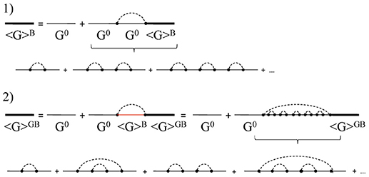
Figure 1. (1) Feynman diagrams representation of the Dyson equation in the Born Approximation. (2) Feynman diagrams representation of the Dyson equation in the next order approximation of the perturbative series expansion, corresponding to truncation of the SCBA to the second step. It represents the starting point of the GBA.

FIGURE 2

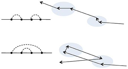
Figure 2. Selection of two Feynman diagrams with the corresponding scattering events. Both the diagrams describe a four-fold scattering. The diagram on the top accounts for double scatterings occuring in the same inhomogeneity, whereas the diagram on the bottom also accounts for a double scattering from two different inhomogeneities.

Depolarization effects in the scattering of electromagnetic waves by an isotropic random medium has been predicted by exploiting a second order representation for the scattered intensity [42]. The scattering of electromagnetic waves by the random media is cast in terms of Green's dyadic and the formal solution of the problem is given in terms of a Neumann iteration series. The n-th order of the scattered intensity is obtained by truncation of the Neumann series and ensemble averaging. Depolarization effects are also observable even in the first-order scattered intensity from an anisotropic random medium [43]. We recall that the optical theorem establish a connection between the self-energy and the intensity operator characterizing the Bethe-Salpter equation, which permits to describe the intensity of the mean field [25]. These results thus emphasize the soundness of our findings.

The input parameters of the theory are the correlation length, a, the disorder parameter, ${\widetilde{ϵ}}^2$, and the longitudinal and transverse phase velocity of the “bare” medium, $c_{L(T)}^0$.

3. Results and Discussion

3.1. The Generalized Born Approximation

Under the hypothesis of local isotropy it is convenient to introduce the orthonormal basis defined by the direction of wave propagation, $\widehat{q}$, and the two orthogonal ones [27]. On this basis all the “bare” Green's dyadic, average Green's dyadic and self-energy are diagonal. The “bare” Green's dyadic becomes

$\begin{array}{cc}\begin{array}{r}{\text{G}}^0(\text{q},\omega )=g_L^0(\text{q},\omega )\widehat{q}\widehat{q}+g_T^0(\text{q},\omega )(I-\widehat{q}\widehat{q}),\end{array}& (10)\end{array}$

with “T” and “L” labeling transverse and longitudinal modes, respectively. The longitudinal and transverse “bare” Green's functions, $g_L^0(\text{q},\omega )$ and $g_T^0(\text{q},\omega )$ respectively, can be formally written by following a regularization procedure [44] as

$\begin{array}{cc}\begin{array}{l}{g}_{L(T)}^0(q,\omega )=li{m}_{\eta \to 0^{+}}\frac{1}{{(\omega +i{c}_{L(T)}^0\eta )}^2-{(c_{L(T)}^{0}q)}^2}\\ ={\left(c_{L(T)}^0\right)}^{-2}p.v.\left\{\frac{1}{q_{0L(T)}^2-q^2}\right\}-i\pi {\left(c_{L(T)}^0\right)}^{-2}·\\ ·\mathrm{sgn}(q_{0L(T)})\delta (q_{0L(T)}^2-q^2),\end{array}& (11)\end{array}$

where $q_{0L(T)}=\frac{\omega }{c_{L(T)}^0}$. In Equation (12) η is a positive real variable, the symbol p.v. states for the Cauchy principal value and sgn(x) is the sign function of argument x. The retarded solution is selected as required by the causality principle [45]. Furthermore,

$\begin{array}{cc}\begin{array}{ll}\Sigma (q,\omega )\hfill & ={\Sigma }_L(q,\omega )\widehat{q}\widehat{q}+{\Sigma }_T(q,\omega )(I-\widehat{q}\widehat{q});\hfill \\ <G(q,\omega )>\hfill & =<g_L(q,\omega )>\widehat{q}\widehat{q}+<g_T(q,\omega )>(I-\widehat{q}\widehat{q}),\hfill \end{array}& (12)\end{array}$

with

$\begin{array}{cc}\begin{array}{r}<g_{L(T)}(\text{q},\omega )>=\frac{1}{g_{L(T)}^0{(\text{q},\omega )}^{-1}-{\Sigma }_{L(T)}(\text{q},\omega )}.\end{array}& (13)\end{array}$

The GBA address an approximate expression of the self-energy obtained by truncation of the perturbative series expansion to the second order. This is obtained by substituting the “bare” Green's dyadics in Equation (8) (Born Approximation) with the expression of the average Green's dyadic obtained by the Born Approximation [25]. It is thus equivalent to truncate Equation 9 to the second iteration step. We obtain for the diagonal terms of the self-energy,

$\begin{array}{cc}\begin{array}{l}{\Sigma }_{kk}(q,\omega )={\widehat{L}}_{1kkii}<G_{ii}(q,\omega ){>}^1\\ ={\widehat{L}}_{1kkii}\frac{1}{{\tilde{c}}_i^2}li{m}_{\eta \to 0^{+}}\left\{\frac{1}{{\tilde{q}}_{0i,\eta }^2-q^2-\frac{{ϵ}^2}{{\tilde{c}}_i^2}{q}^2\Delta {\tilde{\Sigma }}_{ii}^1(q,{\omega }_{\eta })}\right\},\end{array}& (14)\end{array}$

where ${\tilde{q}}_{0i,\eta }=\frac{{\omega }_{\eta }}{{\tilde{c}}_i}$, ${\omega }_{\eta }=\omega +i{\tilde{c}}_i\eta$, ${\tilde{q}}_{0i}=\frac{\omega }{{\tilde{c}}_i}$, ${\omega }_{\eta }=\omega +i{\tilde{c}}_i\eta$ ${\tilde{c}}_i={\left[c_i^2+{ϵ}^2{\tilde{\Sigma }}_i^1\left(q=0,\omega =0\right)\right]}^{1/2}$ is the macroscopic velocity of the (first step) perturbed medium, $\Delta {\tilde{\Sigma }}_{ii}^1(\text{q},\omega )={\tilde{\Sigma }}_{ii}^1(\text{q},\omega )-{\tilde{\Sigma }}_{ii}^1(0,0)$ and ${\tilde{\Sigma }}_{ii}^1(\text{q},\omega )={({ϵ}^2{q}^2)}^{-1}{\Sigma }_{ii}^1(\text{q},\omega )$. The suffix 1 marks a quantity calculated to the first step of the self-consistent procedure. The repeated indexes kk, ii = L, T. The longitudinal and transverse self-energy are thus respectively composed by two terms accounting for the coupling with longitudinal and transverse dynamics respectively, i.e., Σ_L(T) = Σ_LL(TT)+Σ_LT(TL).

The expression in curly bracket in Equation (16), $<G_{ii}(\text{q},\omega ){>}^1$, is then formally expanded in a Taylor series with respect to $\frac{{ϵ}^2}{{\tilde{c}}_i^2}{q}^2\Delta {\tilde{\Sigma }}_{ii}^1(\text{q},{\omega }_{\eta })$. Theorem I below states that this series is convergent almost everywhere (a.e.) in the domain of the (ω, q) plane where the conditions $\frac{{ϵ}^2}{{\tilde{c}}_i^2}\left|\Delta {\tilde{\Sigma }}_{ii}^1(\text{q},\omega )\right|<1$ and $\text{Im}\left[\Delta {\tilde{\Sigma }}_{ii}^1(\text{q},\omega )\right]>0$ are fulfilled. Once identified such a domain, we can then possibly find a sub-domain, as specified in Corollary II, where

$\begin{array}{cc}\begin{array}{l}{\Sigma }_{kk}(q,\omega )~li{m}_{\eta \to 0^{+}}\frac{1}{{\tilde{c}}_i^2}{\displaystyle \sum _{n=0}^{\infty }{\widehat{\text{L}}}_{1kkii}}\\ \left\{\frac{{[\frac{{ϵ}^2}{{\tilde{c}}_i^2}{q}^2\Delta {\tilde{\Sigma }}_{ii}^1(q,{\omega }_{\eta })]}^n}{{[{\tilde{q}}_{0i,\eta }^2-q^2]}^{n+1}}\theta (q_{Max}^i-q)\right\},\end{array}& (15)\end{array}$

θ(x) being the Heaviside function of argument x and $q_{Max}^i$ representing the q-boundary of the domain of convergence of the series representation of $<G_{ii}(\text{q},\omega ){>}^1$. Equation (15) provides the expression of the self-energy in the GBA.

The wavevector-dependence of $\Delta {\tilde{\Sigma }}_{ii}^1(\text{q},\omega )$ is determined by the covariance function used to statistically describe the elastic heterogeneity of the system, as established in Equation (9) above. We analyze in detail the case of an exponential decay of the covariance function with correlation length a and amplitude ϵ². This choice grounds on simplicity and on the fact that several systems can be described by such a covariance function [46]. We show in section 3.2, in particular, that in this case the domain of validity of the GBA includes the region aq ~ 1, where the mixing of polarization is expected.

3.1.1. Series Representation of < G(q, ω) >¹

In the following we demonstrate that it exists a domain of the (ω, q) plane, where the function < G(q, ω) >¹ admits a.e. the power series expansion specified in the following Theorem I.

Theorem I. If, being q, ω ∈ ℝ,

i) $\left|\Delta {\tilde{\Sigma }}_{ii}^1(\text{q},\omega )\right|\in C^0$;

ii) $\left|\Delta {\tilde{\Sigma }}_{ii}^1(\text{q},\omega )\right|\le \Delta {\tilde{\Sigma }}_i^{1,Max}(\omega )$, $q\in \left[0,q_{Max}^i\right]$, eventually $q_{Max}^i\to$ ∞;

iii) $\text{Im}\left[\Delta {\tilde{\Sigma }}_{ii}^1(\text{q},\omega )\right]>0$, ∀q, ω≠0;

for $q_{Max}^i$, ω and ϵ²: ω≠0, $\frac{{ϵ}^2}{{\tilde{c}}_i^2}\Delta {\tilde{\Sigma }}_i^{1,Max}(\omega )<1$, the series $li{m}_{\eta \to 0^{+}}\sum _{n=0}^{\infty }\frac{{\left[\frac{{ϵ}^2}{{\tilde{c}}_i^2}{q}^2\Delta {\tilde{\Sigma }}_{ii}^1(\text{q},{\omega }_{\eta })\right]}^n}{{({\tilde{q}}_{0i,\eta }^2-q^2)}^{n+1}}$ converges a. e. in the q-interval $\left[0,q_{Max}^i\right]$ to the function $li{m}_{\eta \to 0^{+}}\frac{1}{{\tilde{q}}_{0i,\eta }^2-q^2-\frac{{ϵ}^2}{{\tilde{c}}_i^2}{q}^2\Delta {\tilde{\Sigma }}_{ii}^1(\text{q},{\omega }_{\eta })}$.

Before to proceede with the proof, we observe that Theorem I can be applied to cases easily realizable by real systems. Because $\text{Im}\left[\Delta {\tilde{\Sigma }}_{ii}^1(\text{q},\omega )\right]$ is proportional to the attenuation of the acoustic excitations in the random medium calculated to the first order of the perturbative series expansion, in point iii) it is required that such an attenuation is finite for finite values of q and ω. Furthermore, the series a. e. convergence is ensured in a region of wavevectors where the acoustic excitations in the random medium can still be described through a finite and sufficiently small correction with respect to the acoustic excitations in the “bare” medium, being there the self-energy sufficiently small.

From the algebraic equality $\frac{1}{A-B}=\frac{1}{A}+\frac{1}{A}\frac{B}{A-B}$, it follows that

$\begin{array}{l}li{m}_{\eta \to 0^{+}}{\displaystyle {\int }_0^{q_{Max}^i}d}q\frac{1}{{\tilde{q}}_{0i,\eta }^2-q^2-\frac{{ϵ}^2}{{\tilde{c}}_i^2}{q}^2\Delta {\tilde{\Sigma }}_{ii}^1(q,{\omega }_{\eta })}\\ ={\sum }_{n=0}^{N}li{m}_{\eta \to 0^{+}}{\displaystyle {\int }_0^{q_{Max}^i}d}q\frac{{[\frac{{ϵ}^2}{{\tilde{c}}_i^2}{q}^2\Delta {\tilde{\Sigma }}_{ii}^1(q,{\omega }_{\eta })]}^n}{{({\tilde{q}}_{0i,\eta }^2-q^2)}^{n+1}}+R_N^i.\end{array}$

The remainder function is defined as

$li{m}_{\eta \to 0^{+}}{\displaystyle {\int }_0^{q_{Max}^i}d}q\frac{1}{{\tilde{q}}_{0i,\eta }^2-q^2-\frac{{ϵ}^2}{{\tilde{c}}_i^2}{q}^2\Delta {\tilde{\Sigma }}_{ii}^1(q,{\omega }_{\eta })}={\sum }_{n=0}^{N}li{m}_{\eta \to 0^{+}}{\displaystyle {\int }_0^{q_{Max}^i}d}q\frac{{[\frac{{ϵ}^2}{{\tilde{c}}_i^2}{q}^2\Delta {\tilde{\Sigma }}_{ii}^1(q,{\omega }_{\eta })]}^n}{{({\tilde{q}}_{0i,\eta }^2-q^2)}^{n+1}}+R_N^i.$

We demonstrate in the following that $\left|R_N^i\right|$ admits an upper bound, i.e.

$\begin{array}{cc}\begin{array}{l}\left|R_N^i\right|\le M_{i}li{m}_{\eta \to 0^{+}}{\displaystyle {\int }_0^{q_{Max}^i}d}q\frac{{\left[\frac{{ϵ}^2}{{\tilde{c}}_i^2}{q}^2\Delta {\tilde{\Sigma }}_i^{1,Max}(\omega )\right]}^N}{|{\tilde{q}}_{0i,\eta }^2-q^2{|}^{N+1}}\\ \le M_i{\left[\frac{{ϵ}^2}{{\tilde{c}}_i^2}\Delta {\tilde{\Sigma }}_i^{1,Max}(\omega )\right]}^N\frac{N+1}{2N+1}\frac{\pi }{{\tilde{q}}_{0i}},\end{array}& (16)\end{array}$

where $M_i=\underset{q\in \left[0,q_{Max}^i\right]}{sup}\left|\frac{\frac{{ϵ}^2}{{\tilde{c}}_i^2}{q}^2\Delta {\tilde{\Sigma }}_{ii}^1(\text{q},\omega )}{{\tilde{q}}_{0i}^2-q^2-\frac{{ϵ}^2}{{\tilde{c}}^2}{q}^2\Delta {\tilde{\Sigma }}_{ii}^1(\text{q},\omega )}\right|$. The latter quantity exists as a consequence of the hypotheses of Theorem I. It is indeed immediate to recognize that for q, ω ∈ ℝ and ω ≠ 0, if $\text{Im}\left[\Delta {\tilde{\Sigma }}_{ii}^1(\text{q},\omega )\right]$ is strictly positive, the function $\frac{1}{{\tilde{q}}_{0i}^2-q^2-\frac{{ϵ}^2}{{\tilde{c}}_i^2}{q}^2\Delta {\tilde{\Sigma }}_{ii}(\text{q},\omega )}$ is bounded, do not having poles.

To prove the inequality in the third side of Equation (18) we need to show that

$\begin{array}{cc}li{m}_{\eta \to 0^{+}}{\displaystyle {\int }_0^{q_{Max}^i}d}q\frac{{[q^2]}^N}{|{({\tilde{q}}_{0i}+i\eta )}^2-q^2{|}^{N+1}}\le \frac{(N+1)}{(2N+1)}\frac{\pi }{{\tilde{q}}_{0i}},& (17)\end{array}$

where for sake of simplicity we renamed the variable $\frac{\eta }{{\tilde{c}}_i}$ as η. We discuss only the case ${\tilde{q}}_{0i}<q_{Max}^i$. The case ${\tilde{q}}_{0i}>q_{Max}^i$ can be easily reconducted to the former by noticing that ${\displaystyle {\int }_0^{q_{Max}^i}d}q\frac{{[q^2]}^N}{|{({\tilde{q}}_{0i}+i\eta )}^2-q^2{|}^{N+1}}\le {\displaystyle {\int }_0^{\infty }d}q\frac{{[q^2]}^N}{|{({\tilde{q}}_{0i}+i\eta )}^2-q^2{|}^{N+1}}$.

We observe that

$\begin{array}{cc}\begin{array}{r}\frac{1}{2}\left[\frac{1}{z^N}+\frac{1}{{\overline{z}}^N}\right]=\frac{cos(N\theta )}{|z{|}^N};\frac{1}{2}\left[\frac{1}{z^N}-\frac{1}{{\overline{z}}^N}\right]=-i\frac{sin(N\theta )}{|z{|}^N},\end{array}& (18)\end{array}$

where z is a generic complex variable, $\overline{z}$ is its complex conjugate and θ = arg(z). Furthermore

$\begin{array}{cc}\begin{array}{l}\frac{1}{|z{|}^N}\le \frac{|\cos (N\theta )|}{|z{|}^N}+\frac{|\sin (N\theta )|}{|z{|}^N}\\ =\frac{1}{2}\mathrm{sgn}\{\cos (N\theta )\}\left[\frac{1}{z^N}+\frac{1}{{\overline{z}}^N}\right]\\ +\frac{1}{2}i\mathrm{sgn}\{\sin (N\theta )\}\left[\frac{1}{z^N}-\frac{1}{{\overline{z}}^N}\right].\end{array}& (19)\end{array}$

The inequality $1={\left[{sin}^2(x)+{cos}^2(x)\right]}^{\frac{1}{2}}\le |sin(x)|+|cos(x)|$ has been exploited. We furthermore considered that |cos(x)| = cos(x)·sgn{cos(x)}. The same applies to sin(x). It is thus

$\begin{array}{cc}\begin{array}{l}li{m}_{\eta \to 0^{+}}{\displaystyle {\int }_0^{q_{Max}^i}d}q\frac{{[q^2]}^N}{|q^2-{({\tilde{q}}_{0i}+i\eta )}^2{|}^{N+1}}\\ \le \frac{1}{2}li{m}_{\eta \to 0^{+}}{\displaystyle {\int }_0^{q_{Max}^i}d}q[\frac{{[q^2]}^N}{{[q^2-{({\tilde{q}}_{0i}+i\eta )}^2]}^{N+1}}\\ +\frac{{[q^2]}^N}{{[q^2-{({\tilde{q}}_{0i}-i\eta )}^2]}^{N+1}}]\mathrm{sgn}\{\cos [(N+1)\theta (\eta )]\}\\ +\frac{1}{2}ili{m}_{\eta \to 0^{+}}{\displaystyle {\int }_0^{q_{Max}^i}d}q[\frac{{[q^2]}^N}{{[q^2-{({\tilde{q}}_{0i}+i\eta )}^2]}^{N+1}}\\ -\frac{{[q^2]}^N}{{[q^2-{({\tilde{q}}_{0i}-i\eta )}^2]}^{N+1}}]\mathrm{sgn}\{\sin [(N+1)\theta (\eta )]\},\end{array}& (20)\end{array}$

where $\theta (\eta )=arg\left\{q^2-{({\tilde{q}}_{0i}+i\eta )}^2\right\}$. In the framework of a generalization of the Sokhotski-Plemelj theorem [47] due to Fox [48] it is possible to show that [49]

$\begin{array}{cc}li{m}_{\eta \to 0^{+}}{\displaystyle {\int }_a^{b}d}x\frac{f(x)}{{[x-(x_0\mp i\eta )]}^{N+1}}={\displaystyle {\int }_{{\gamma }^{\pm }(x_0)}d}z\frac{f(z)}{{(z-x_0)}^{N+1}},& (21)\end{array}$

where a, b, x₀ and x are real variables: a < x₀ < b, f(x) is a function which admits a complex extension f(z) that is analytic in a region of the complex plane containing the interval [a, b] but not x₀, R_x0 = R\{x₀}, ${\gamma }^{\pm }(x_0)$ is a path of the region R_x0 from a to b belonging to the upper (lower) half-plane of the complex plane. The second side of Equation (20) can thus be rephrased as

$\begin{array}{cc}\begin{array}{l}\frac{1}{2}\left({\displaystyle {\int }_{{\gamma }^{-}({\tilde{q}}_{0i})}\mathrm{sgn}}\{\cos [(N+1)\theta ]\}+{\displaystyle {\int }_{{\gamma }^{+}({\tilde{q}}_{0i})}\mathrm{sgn}}\{\cos [(N+1)\overline{\theta }]\}\right)dz\\ \frac{{[z^2]}^N}{{(z^2-{\tilde{q}}_{0i}^2)}^{N+1}}+\frac{1}{2}i({\displaystyle {\int }_{{\gamma }^{-}({\tilde{q}}_{0i})}\mathrm{sgn}}\{\sin [(N+1)\theta ]\}\\ -{\displaystyle {\int }_{{\gamma }^{+}({\tilde{q}}_{0i})}\mathrm{sgn}}\{\sin [(N+1)\overline{\theta }]\})dz\frac{{[z^2]}^N}{{(z^2-{\tilde{q}}_{0i}^2)}^{N+1}}=\\ =\#{\displaystyle {\int }_0^{q_{Max}^i}d}q\frac{{[q^2]}^N}{{(q^2-{\tilde{q}}_{0i}^2)}^{N+1}}+\pi \frac{1}{N!}\frac{d^N}{d{z}^N}\frac{{[z^2]}^N}{{(z+{\tilde{q}}_{0i})}^{N+1}}{|}_{z={\tilde{q}}_{0i}},\end{array}& (22)\end{array}$

where ${\gamma }^{\pm }({\tilde{q}}_{0i})$ is the contour of the upper (lower) complex half-plane obtained by deformation of the segment $\left[0,q_{Max}^i\right]$ around ${\tilde{q}}_{0i}$ by an infinitesimal arc of circle of radius ϕ passing around ${\tilde{q}}_{0i}$ clockwise (counterclockwise). Furthermore it is $\theta =Arg(z^2-{\tilde{q}}_{0i}^2)$ and $\overline{\theta }=Arg({\overline{z}}^2-{\tilde{q}}_{0i}^2)$. The symbol # denotes the Hadamard Finite-Part Integrals (or Cauchy Principal Value when N = 0) [47–49]. We observe that i) $\overline{\theta }=-\theta$; ii) for z∈ℝ it is $\theta =\overline{\theta }=0$; iii) for z∈ℂ it is $\mathrm{\text{sgn}}\left\{sin\left[(N+1)\overline{\theta }\right]\right\}{|}_{z\in {\gamma }^{+}({\tilde{q}}_{0i})}=\mathrm{\text{sgn}}\left\{sin\left[(N+1)\theta \right]\right\}{|}_{z\in {\gamma }^{-}({\tilde{q}}_{0i})}$, $\mathrm{\text{sgn}}\left\{cos\left[(N+1)\overline{\theta }\right]\right\}{|}_{z\in {\gamma }^{+}({\tilde{q}}_{0i})}=\mathrm{\text{sgn}}\left\{cos\left[(N+1)\theta \right]\right\}{|}_{z\in {\gamma }^{-}({\tilde{q}}_{0i})}$. The last passage in Equation (22) follows from (i) the fact that [49]

$\begin{array}{cc}\begin{array}{l}\frac{1}{2}\left({\displaystyle {\int }_{{\gamma }^{+}(x_0)}d}z\frac{f(z)}{{(z-x_0)}^{N+1}}+{\displaystyle {\int }_{{\gamma }^{-}(x_0)}d}z\frac{f(z)}{{(z-x_0)}^{N+1}}\right)\\ =\#{\displaystyle {\int }_a^{b}d}x\frac{f(x)}{{(x-x_0)}^{N+1}},n\end{array}& (23)\end{array}$

and ii) from the Residue Theorem,

$\begin{array}{cc}\begin{array}{l}{\displaystyle {\int }_{{\gamma }^{-}(x_0)}d}z\frac{f(z)}{{(z-x_0)}^{N+1}}-{\displaystyle {\int }_{{\gamma }^{+}(x_0)}d}z\frac{f(z)}{{(z-x_0)}^{N+1}}\\ =2\pi iRe{s}^{(N+1)}[f(z),x_0]\\ =2\pi i\frac{1}{N!}\frac{d^N}{d{z}^N}[f(z){\left(z-x_0\right)}^{N+1}]{|}_{z=x_0},\end{array}& (24)\end{array}$

where $Re{s}^{(N)}\left[f(z),x_0\right]$ is the residue of order N of the function f(z) around the pole at z = x₀ enclosed in the closed path of the complex plane ${\gamma }^{-}(x_0)-{\gamma }^{+}(x_0)$. It is

$\begin{array}{cc}\#{\displaystyle {\int }_0^{q_{Max}^i}d}q\frac{{[q^2]}^N}{{(q^2-{\tilde{q}}_{0i}^2)}^{N+1}}\le \#{\displaystyle {\int }_0^{\infty }d}q\frac{{[q^2]}^N}{{(q^2-{\tilde{q}}_{0i}^2)}^{N+1}}.& (25)\end{array}$

Using integration by parts and the Stokes' formula one obtains [50]

$\begin{array}{cc}\begin{array}{l}\#{\displaystyle {\int }_0^{\infty }d}q\frac{{[q^2]}^N}{{(q^2-{\tilde{q}}_{0i}^2)}^{N+1}}=p.v.{\displaystyle {\int }_0^{\infty }d}q\frac{1}{q-{\tilde{q}}_{0i}}\frac{1}{N!}\frac{d^N}{d{q}^N}\\ \left[\frac{{[q^2]}^N}{{(q+{\tilde{q}}_{0i})}^{N+1}}\right].\end{array}& (26)\end{array}$

The latter equality ensures the existence of the Hadamard Finite-Part Integral, because the Cauchy p.v. exists as a consequence of the fact that, the N-th order derivative of the function $\frac{{\left[q^2\right]}^N}{{(q+{\tilde{q}}_{0i})}^{N+1}}$ satisfies the Lipschitz condition. It is possible to exploit the Residue Theorem to calculate the integral in Equation (30) and verify that such an integral is equal to zero. In Appendix B, we furthermore prove that

$\begin{array}{cc}\begin{array}{rcl}\frac{1}{N!}\frac{d^N}{d{z}^N}\left[f(z){(z-x_0)}^{N+1}\right]{|}_{z=x_0}& =& \frac{N+1}{2N+1}\frac{1}{{\tilde{q}}_{0i}},\end{array}& (27)\end{array}$

The validity of Equation (17) hence follows from Equation (22).

From Equation (16), we can finally conclude that if $\frac{{ϵ}^2}{{\tilde{c}}_i^2}\Delta {\tilde{\Sigma }}_i^{1,Max}(\omega )<1$ and ω≠0, it is $li{m}_{N\to \infty }\left|R_N^i\right|=0$. Under these conditions we proved that

$\begin{array}{cc}\begin{array}{l}li{m}_{\eta \to 0^{+}}{\displaystyle {\int }_0^{q_{Max}^i}d}q\frac{1}{{\tilde{q}}_{0i,\eta }^2-q^2-\frac{{ϵ}^2}{{\tilde{c}}_i^2}{q}^2\Delta {\tilde{\Sigma }}_{ii}^1(q,{\omega }_{\eta })}\\ ={\displaystyle \sum _{n=0}^{\infty }l}i{m}_{\eta \to 0^{+}}{\displaystyle {\int }_0^{q_{Max}^i}d}q\frac{{[\frac{{ϵ}^2}{{\tilde{c}}_i^2}{q}^2\Delta {\tilde{\Sigma }}_{ii}^1(q,{\omega }_{\eta })]}^n}{{({\tilde{q}}_{0i,\eta }^2-q^2)}^{n+1}},\end{array}& (28)\end{array}$

thus finally proving [51] Theorem I .

3.1.2. Validity of the Generalized Born Approximation

It is worth at this point to provide the expression for the operator ${\widehat{\text{L}}}_1$, starting from Equation (8), under the hypothesis of local isotropy in the orthonormal basis defined above. By performing appropriate inner product on the tensor $\tilde{\text{R}}(\text{q})$, it is obtained [27],

$\begin{array}{cc}\begin{array}{l}{\Sigma }_{kk}(q,\omega )={\widehat{L}}_{1kkii}<G_{ii}(q,\omega ){>}^1\\ ={ϵ}^2{q}^2{\displaystyle \int d}{q}^{\prime }c(|q-q^{\prime }|)L_{kkii}(\widehat{q{q}^{\prime }})<G_{ii}(q^{\prime },\omega ){>}^1,\end{array}& (29)\end{array}$

where c(q) is the scalar covariance function of the elastic constants fluctuations, real and positive-defined [46]; $L_{kkii}(\widehat{q{q}^{\prime }})$ is a function of the angle $\widehat{q{q}^{\prime }}$ between the two versors $\widehat{q}$ and ${\widehat{q}}^{\prime }$, resulting from the inner product [23, 27] also accounting for the transverse degeneracy. The assumption of isotropy allows this function to depend only on the angle $\widehat{q{q}^{\prime }}$. By making use of spherical coordinates we finally achieve

$\begin{array}{cc}\begin{array}{r}{\displaystyle \underset{0}{\overset{\infty }{\int }}}d{q}^{\prime }{q{}^{\prime }}^{2}c(q,q^{\prime },x)<G_{ii}({\text{q}}^{\prime },\omega ){>}^1,\end{array}& (30)\end{array}$

with $x=cos(\widehat{q{q}^{\prime }})$. The function ${\tilde{\Sigma }}_{kk}(\text{q},\omega )$ is implicitly defined in Equation (30).

The validity of the Generalized Born Approximation follows from the following two corollaries of Theorem I.

Corollary I. If the covariance function c(q, q′, x)∈C⁰ for $q^{\prime }\in \left[0,q_{Max}^i\right]$, then

$\begin{array}{cc}\begin{array}{l}li{m}_{\eta \to 0^{+}}{\displaystyle {\int }_0^{q_{Max}^i}d}{q}^{\prime }{q^{\prime }}^{2}c(q,q^{\prime },x)\frac{1}{{\tilde{q}}_{0i,\eta }^2-{q^{\prime }}^2-\frac{{ϵ}^2}{{\tilde{c}}_i^2}{q^{\prime }}^2\Delta {\tilde{\Sigma }}_{ii}^1(q^{\prime },{\omega }_{\eta })}\\ ={\displaystyle \sum _{n=0}^{\infty }l}i{m}_{\eta \to 0^{+}}{\displaystyle {\int }_0^{q_{Max}^i}d}{q}^{\prime }{q^{\prime }}^{2}c(q,q^{\prime },x)\frac{{[\frac{{ϵ}^2}{{\tilde{c}}_i^2}{q^{\prime }}^2\Delta {\tilde{\Sigma }}_{ii}^1(q^{\prime },{\omega }_{\eta })]}^n}{{({\tilde{q}}_{0i,\eta }^2-{q^{\prime }}^2)}^{n+1}}.\end{array}& (31)\end{array}$

The function q^′2c(q, q′, x) for x∈[−1, 1] and $q^{\prime }\in \left[0,q_{Max}^i\right]$ is continuous and bounded. Corollary I thus follows immediately from Theorem I.

We recast the function ${\tilde{\Sigma }}_{kk}(\text{q},\omega )$ in Equation (35) as

$\begin{array}{cc}\begin{array}{l}{\tilde{\Sigma }}_{kk}(q,\omega )={\displaystyle {\int }_{-1}^{1}d}x{L}_{kkii}(x)\frac{2\pi }{{\tilde{c}}_i^2}{\displaystyle {\int }_0^{q_{Max}^i}d}{q}^{\prime }{q^{\prime }}^{2}c(q,q^{\prime },x)\\ \frac{1}{{\tilde{q}}_{0i}^2-{q^{\prime }}^2-\frac{{ϵ}^2}{{\tilde{c}}_i^2}{q^{\prime }}^2\Delta {\tilde{\Sigma }}_{ii}^1(q^{\prime },\omega )}+{\tilde{R}}_k(q,\omega ,{ϵ}^2),\end{array}& (32)\end{array}$

where the remainder function, ${\tilde{R}}_k(\text{q},\omega ,{ϵ}^2)$, is

$\begin{array}{cc}\begin{array}{r}{q{}^{\prime }}^{2}c(q,q^{\prime },x)\frac{{\left[\frac{{ϵ}^2}{{\tilde{c}}_i^2}{q{}^{\prime }}^2\Delta {\tilde{\Sigma }}_{ii}^1({\text{q}}^{\prime },\omega )\right]}^n}{{({\tilde{q}}_{0i,\eta }^2-{q{}^{\prime }}^2)}^{n+1}}.\end{array}& (33)\end{array}$

Corollary II. For those values of ϵ², q and ω: $|{\tilde{R}}_k(q,\omega ,{ϵ}^2)|\ll 1$, it is

$\begin{array}{cc}\begin{array}{l}{\tilde{\Sigma }}_{kk}(q,\omega )~{\displaystyle \sum _{n=0}^{\infty }{F}_k^n}(q,\omega )=\\ ={\displaystyle \sum _{n=0}^{\infty }l}i{m}_{\eta \to 0^{+}}{\displaystyle {\int }_{-1}^{1}d}x{L}_{kkii}(x)\frac{2\pi }{{\tilde{c}}_i^2}{\displaystyle {\int }_0^{q_{Max}^i}d}{q}^{\prime }\\ {q^{\prime }}^{2}c(q,q^{\prime },x)\frac{{[\frac{{ϵ}^2}{{\tilde{c}}_i^2}{q^{\prime }}^2\Delta {\tilde{\Sigma }}_{ii}^1(q^{\prime },\omega )]}^n}{{({\tilde{q}}_{0i,\eta }^2-{q^{\prime }}^2)}^{n+1}}.\end{array}& (34)\end{array}$

The generic term of the series, $F_k^n(\text{q},\omega )$, is implicitly defined in Equation (34). Corollary II follows from Corollary I. We emphasize, furthermore, that the validity of of Corollary II is constraint to the assumption of negligible contribution of the self-energy to the average Green's dyadic if $\frac{{ϵ}^2}{{\tilde{c}}_i^2}\frac{\left|{\Sigma }_{kk}(\text{q},\omega )\right|}{q^2}\ll 1$. Corollary II is, however, still valid when this hypothesis is violated but it is possible to show that $\left|{\tilde{R}}_k(\text{q},\omega ,{ϵ}^2)\right|\ll \left|\underset{-1}{\overset{1}{\int }}dx{L}_{kkii}(x)\frac{2\pi }{{\tilde{c}}_i^2}\underset{0}{\overset{q_{Max}^i}{\int }}d{q}^{\prime }{q{}^{\prime }}^{2}c(q,q^{\prime },x)\frac{1}{{\tilde{q}}_{0i}^2-{q{}^{\prime }}^2-\frac{{ϵ}^2}{{\tilde{c}}_i^2}{q{}^{\prime }}^2\Delta {\tilde{\Sigma }}_{ii}^1({\text{q}}^{\prime },\omega )}\right|$.

3.2. The Case of an Exponential Decay of the Covariance Function

We analyze in detail the case of a covariance function cast in the form of an exponential decay function, finding the domain of validity of the GBA in the (ω, q) plane. We furthermore consider only spatial fluctuations of the shear modulus. The results, however, can be easily generalized by including also spatial fluctuations of the Lamé parameter [27].

In a three-dimensional Fourier space the covariance function in this case reads as

$\begin{array}{cc}c(q)=\frac{1}{{\pi }^2}\frac{q^2{a}^{-1}}{{(q^2+a^{-2})}^2},& (35)\end{array}$

where ∫d³q c(q) = 1. Furthermore it is ${ϵ}^2={\widetilde{ϵ}}^2{\mu }_0^2=\delta {\mu }^2$, being δμ the intensity of the spatial fluctuations of the shear modulus per density. From Equation (35) we obtain that in Equation (30) it is $c(q,q^{\prime },x)=\frac{a}{{\pi }^2}\frac{{(a{q}^{\prime })}^2}{{(1+{(a{q}^{\prime })}^2+{(aq)}^2-2(a{q}^{\prime })(aq)x)}^2}$.

We first verify in the following that the hypotheses of Theorem I are verified when the covariance function is given by Equation (35). The validity of Corollary I follows immediately from the continuity of the function in Equation (35). It is finally possible to find a domain of the (ω, q) plane where Corollary II holds. In this domain the GBA can be exploited. It covers a q-range up to ~a⁻¹.

We show that in the case of an exponential decay of the covariance function , as required by the hypotheses of Theorem I, for q, ω∈ℝ, i) $\left|\Delta {\tilde{\Sigma }}_{ii}^1(\text{q},\omega )\right|$ is continuous and bounded for $q\in \left[0,q_{Max}^i\right]$, $\exists q_{Max}^i$ ∀i; ii) $\text{Im}\left[\Delta {\tilde{\Sigma }}_{ii}^1(\text{q},\omega )\right]>0$, The self-energy in the Born Approximation,

$\begin{array}{cc}{\tilde{\Sigma }}_{ii}^1(q,\omega )={\displaystyle {\int }_{-1}^{1}d}x{L}_{iijj}(x)\frac{2\pi }{c_j^2}li{m}_{\eta \to 0^{+}}{\displaystyle {\int }_0^{\infty }d}{q}^{\prime }{q^{\prime }}^{2}c(q,q^{\prime },x)\frac{1}{q_{0j,\eta }^2-{q^{\prime }}^2},& (36)\end{array}$

can in such a case be calculated by exploiting the Sokhotski-Plemelj theorem and the Cauchy's Residue Theorem [23, 27], finding

$\begin{array}{cc}\begin{array}{l}{\tilde{\Sigma }}_{ii}^1(q,\omega )=i{\displaystyle {\int }_{-1}^{1}d}x{L}_{iijj}(x)\frac{2}{c_j^2}\frac{{(a{q}_{0j})}^3}{{(1+{(aq)}^2+{(a{q}_{0j})}^2+2(aq)(a{q}_{0j})x)}^2}\\ -{\displaystyle {\int }_{-1}^{1}d}x{L}_{iijj}(x)\frac{2}{c_j^2}\frac{1}{{\tilde{a}}^3}·\{[{\tilde{a}}^{10}+2{\left(aq\right)}^4{x}^4{\left(-{\left(a{q}_{0j}\right)}^2+{\left(aq\right)}^2{x}^2\right)}^3\\ +{\tilde{a}}^8(5{\left(a{q}_{0j}\right)}^2+6{\left(aq\right)}^2{x}^2)+a^6(7{\left(a{q}_{0j}\right)}^4+17{\left(aq\right)}^2{\left(a{q}_{0j}\right)}^2{x}^2\\ +4{\left(aq\right)}^4{x}^4)+{\tilde{a}}^4(3{\left(a{q}_{0j}\right)}^6+16{\left(aq\right)}^2{\left(a{q}_{0j}\right)}^4{x}^2\\ +13{\left(aq\right)}^4{\left(a{q}_{0j}\right)}^2{x}^4+16{\left(aq\right)}^6{x}^6)+{\tilde{a}}^2(-3{\left(aq\right)}^2{\left(a{q}_{0j}\right)}^6{x}^2\\ -{\left(aq\right)}^4{\left(a{q}_{0j}\right)}^4{x}^4-5{\left(aq\right)}^6{\left(a{q}_{0j}\right)}^2{x}^6+9{\left(aq\right)}^8{x}^8)]/\\ {\left[{\tilde{a}}^4+{\left({\left(a{q}_{0j}\right)}^2-{\left(aq\right)}^2{x}^2\right)}^2+2{\tilde{a}}^2{\left({\left(a{q}_{0j}\right)}^2+{\left(aq\right)}^2{x}^2\right)}^2\right]}^2\},\end{array}& (37)\end{array}$

where ã(q, x) = [(1−^{x2)(aq)2+1]1/2} and $L_{LL}(x)=4x^4$, $L_{LT}(x)=4(1-x^2)x^2$, $L_{TT}(x)=\frac{1}{2}(1-3x^2+4x^4)$, $L_{TL}(x)=2(1-x^2)x^2$. The x-integration is performed numerically. Furthermore, it is ${\tilde{\Sigma }}_{ii}^1(0,0)=-\underset{-1}{\overset{1}{\int }}dx\frac{2}{c_j^2}{L}_{iijj}(x)$. From inspection of Equation (44) we deduce that $\text{Im}\left[\Delta {\tilde{\Sigma }}_{ii}^1(\text{q},\omega )\right]>0$; $\left|\Delta {\tilde{\Sigma }}_{ii}^1(\text{q},\omega )\right|\in C^0$ for q, ω∈ℝ.

We define in the following the domain of the (ω, q) plane where Corollary II holds. Specifics of the mathematical passages are outlined in Supplementary Note 1. We first specify the domain of convergence a.e. in the (ω, q) plane of the series representation of $<G_{ii}(\text{q},\omega ){>}^1$. We then show that the magnitude of the remainder function, $\left|{\tilde{R}}_k(\text{q},\omega ,{ϵ}^2)\right|$, is as small as required by Corollary II when $a{q}_{Max}^i$ is large enough. We finally note that such a condition corresponds to deal with small values of $\frac{{ϵ}^2}{{\tilde{c}}_i^2}$.

As we infer from Equation (37) and observe in Figure 3, $\left|\Delta {\tilde{\Sigma }}_{ii}^1(\text{q},\omega )\right|$: i) definitively and independently from ω increases by increasing q with a q² leading term ; ii) it has a local maximum in q~q_0i. The value of this maximum increases by increasing q_0i, as it is possible to observe in Figure 3, Panels 2. It follows from Theorem I that the condition $\frac{{ϵ}^2}{{\tilde{c}}_i^2}\Delta {\tilde{\Sigma }}_i^{1,Max}(\omega )<1$ permits to discriminate the values of q and ω where the series representation of $<G_{ii}(\text{q},\omega ){>}^1$ is a.e. convergent. Given the properties of $\left|\Delta {\tilde{\Sigma }}_{ii}^1(\text{q},\omega )\right|$ stated in points i) and ii) above we infer that this inequality is fulfilled for values of ω and $q\in \left[0,q_{Max}^i\right]$: a) $\frac{{ϵ}^2}{{\tilde{c}}_i^2}\left|\Delta {\tilde{\Sigma }}_{ii}^1(q_{0i},\omega )\right|<1$ and, b) $\frac{{ϵ}^2}{{\tilde{c}}_i^2}\left|\Delta {\tilde{\Sigma }}_{ii}^1(q_{Max}^i,\omega )\right|<1$. We observe that $\left|\Delta {\tilde{\Sigma }}_{ii}^1(q_{0i},\omega )\right|$ increases by increasing q_0i with a $q_{0i}^3$ leading term, see Equation 44. The frequency values where the condition a) is satisfied are thus $q_{0i}=\frac{\omega }{c_i^0}\ll q_{Max}^i$, as it is possible to infer also by the observation of Figure 4. We then fix a value of frequency where the conditions a) and b) are satisfied and observe that for q≫q_0i, i.e., $q~q_{Max}^i$, $\text{Im}\left[\Delta {\tilde{\Sigma }}_{ii}^1(\text{q},\omega )\right]\ll 1$. This is verified in Supplementary Note 1. Consequently, the function $\frac{1}{|{\tilde{q}}_{0i}^2-q^2-\frac{{ϵ}^2}{{\tilde{c}}_i^2}{q}^2\Delta {\tilde{\Sigma }}_{ii}^1(\text{q},\omega )|}$ has a local maximum at ${\overline{q}}^i:\frac{{ϵ}^2}{{\tilde{c}}_i^2}\left|Re\left\{\Delta {\tilde{\Sigma }}_{ii}^1({\overline{\text{q}}}^i,\omega )\right\}\right|=\frac{{{\overline{q}}^i}^2-{\tilde{q}}_{0i}^2}{{{\overline{q}}^i}^2}$. At larger wavevectors this function monotonically decreases by increasing q until to be lower of $\frac{1}{|{\tilde{q}}_{0i}^2-q^2|}$. This behavior can be observed in Figure 4, Panels 3. The trends outlined permit finally to asses that for $q_{0i}\ll q_{Max}^i$ and $q\ll Mi{n}_{\left\{i\right\}}\left[q_{Max}^i\right]$ and for values sufficiently large of $a{q}_{Max}^i$, it is $\left|{\tilde{R}}_k(\text{q},\omega ,{ϵ}^2)\right|\lesssim \sum _i\frac{1}{{\tilde{c}}_i^2}\frac{1}{a{q}_{Max}^i}$. The mathematical passages are shown in detail in Supplementary Note 1. It is thus $\left|{\tilde{R}}_k(\text{q},\omega ,{ϵ}^2)\right|\ll 1$ when $a{q}_{Max}^i$ is large enough. In this case Corollary II holds and we can exploit the GBA. We infer from point i) and observe in Figure 3, Panels 2, that as smaller it is $\frac{{ϵ}^2}{{\tilde{c}}_i^2}$ as larger is $a{q}_{Max}^i$. It furthermore follows that for a given value of ϵ² the larger it is ${\tilde{c}}_i$, the larger $a{q}_{Max}^i$. The magnitude of the remainder function remain thus uniquely linked to the value of $\frac{{ϵ}^2}{{\tilde{c}}_i^2}$. Finally, noting the inverse proportionality between $a{q}_{Max}^i$ and the magnitude of the remainder function, we expect that the domain of the (ω, q) plane where the GBA can be applied includes values of q:aq ~ 1. A specific case is treated in Figures 4–6, where the quantities shown have been obtained for theory's input parameters which allow to describe the features of longitudinal dynamics for a real system [41]. They are $c_L^0=2.29$ meV/nm⁻¹, $c_T^0/c_L^0=0.53$, ${\widetilde{ϵ}}^2=\frac{{ϵ}^2}{{\mu }_0^2}=0.4$ and a = 1.1 nm. By inspection of Figures 4–5 we find $a{q}_{Max}^L=18$, $a{q}_{Max}^T=8$. For such theory's input parameters the GBA hence holds for q:aq≪8. The mixing of polarization is expected for aq~1. In this case the proposed approximation can thus be used to describe such a phenomenon.

FIGURE 3

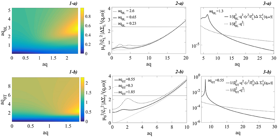
Figure 3. (1) Projection on the (ω, q) plane of a) $\frac{{\mu }_0^2}{{\tilde{c}}_L^2}\left|\Delta {\tilde{\Sigma }}_L^1(\text{q},\omega )\right|$ and b) $\frac{{\mu }_0^2}{{\tilde{c}}_T^2}\left|\Delta {\tilde{\Sigma }}_T^1(\text{q},\omega )\right|$. (2) $\frac{{\mu }_0^2}{{\tilde{c}}_{L(T)}^2}\left|\Delta {\tilde{\Sigma }}_{L(T)}^1(\text{q},\omega )\right|$ as a function of aq for three selected values of aq_0L(T). The straight line fixes the value of ${({\widetilde{ϵ}}^2)}^{-1}$. (3) $\frac{1}{|{\tilde{q}}_{0L(T)}^2-q^2-\frac{{ϵ}^2}{{\tilde{c}}_{L(T)}^2}{q}^2\Delta {\tilde{\Sigma }}_{L(T)}^1(\text{q},\omega )|}$ (black line) and $\frac{1}{|{\tilde{q}}_{0L(T)}^2-q^2|}$ (dashed line) as a function of aq for a given value of aq_0L(T). The covariance function is cast in an exponential decay function. The values of the theory's input parameters are listed in the text.

FIGURE 4

Figure 4. $\frac{{\mu }_0^2}{{\tilde{c}}_{L(T)}^2}\left|\Delta {\tilde{\Sigma }}_L^1(q_{0L(T)},\omega )\right|$ for an exponentially decaying covariance function. The straight line fixes the value of ${({\widetilde{ϵ}}^2)}^{-1}$. The values of the theory's input parameters are listed in the text.

FIGURE 5

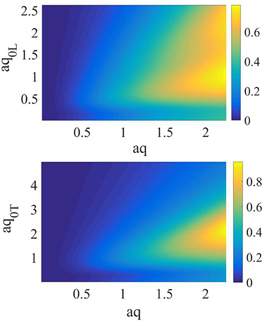
Figure 5. Projection on the (ω, q) plane of $\frac{|\Delta {\tilde{\Sigma }}_L^1(q,\omega )-\Delta {\tilde{\Sigma }}_L^1(0,\omega )|}{\left|\Delta {\tilde{\Sigma }}_L^1(0,\omega )\right|}$ (Left) and $\frac{|\Delta {\tilde{\Sigma }}_T^1(q,\omega )-\Delta {\tilde{\Sigma }}_T^1(0,\omega )|}{\left|\Delta {\tilde{\Sigma }}_T^1(0,\omega )\right|}$ (Right) for an exponential decay of the covariance function. The values of the theory's input parameters are listed in the text.

FIGURE 6

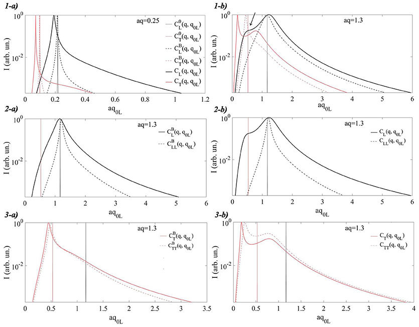
Figure 6. (1) Longitudinal and transverse currents (black and red lines respectively) obtained by exploiting the GBA (full line) and the Born Approximation (dashed line) in the case of an exponential decay of the covariance function for different values of wavevector. The values of the theory's input parameters, listed in the text, are the same for both approximations. (2) Longitudinal currents obtained by exploiting the Born Approximation, a), and the GBA, b). Full lines show the currents obtained by considering the full expression of the self-energy, Σ_L(q, ω), dot-dashed lines show the currents obtained by considering the only longitudinal contribution to the self-energy, Σ_LL(q, ω). (3) Transverse currents obtained by exploiting the Born Approximation, a), and the GBA, b). Full lines show the currents obtained by considering the full expression of the self-energy, Σ_T(q, ω), dot-dashed lines show the currents obtained by considering only the transverse contribution to the self-energy, Σ_TT(q, ω).

For the input parameters specified above we calculate the longitudinal and transverse self-energies in the GBA. In sections 3.3 and 3.4 we analyse the features of the acoustic dynamics focusing, in particular, on the mixing of polarizations. To this aim we truncate the series in Equation (34) to the order n = 1, obtaining ${\Sigma }_{kk}(\text{q},\omega )~F_k^0(\text{q},\omega )+F_k^1(\text{q},\omega )$. In Supplementary Note 2, we numerically retrieve the value of $\left|F_k^1(\text{q},\omega )\right|$ and $\left|{\tilde{R}}_k(\text{q},\omega ,{ϵ}^2)\right|$ for selected values of wavevector and frequency and show that the former is significantly larger than the latter. We notice that the series in Equation (34) is obtained as the integral of a power series a.e. convergent. It is thus expected that the leading-order terms will be the ones with smaller n. Such an order of approximation is furthermore sufficient to obtain a realistic description of the acoustic dynamics, including the Rayleigh anomalies and the mixing of polarizations [41]. In order to facilitate such calculation we furthermore assume $\Delta {\tilde{\Sigma }}_{ii}^1({\text{q}}^{\prime },\omega )~\Delta {\tilde{\Sigma }}_{ii}^1(0,\omega )$. When the approximation $\Delta {\tilde{\Sigma }}_{ii}^1({\text{q}}^{\prime },\omega )~\Delta {\tilde{\Sigma }}_{ii}^1(0,\omega )$ applies, the Hadamard principal value of the integral defining $F_k^1(\text{q},\omega )$ can be obtained straightforwardly by exploiting the Residue Theorem. In such a case we can indeed extend the upper integration boundary of the integral to infinity while maintaining unaffected the order of magnitude of the error related to the GBA, as discussed in Supplementary Note 3. It is furthermore shortly discussed in Supplementary Note 4 that as long as the condition $\left|\frac{\Delta {\tilde{\Sigma }}_{ii}^1({\text{q}}^{\prime },\omega )-\Delta {\tilde{\Sigma }}_{ii}^1(0,\omega )}{\Delta {\tilde{\Sigma }}_{ii}^1(0,\omega )}\right|<\frac{1}{2}$ is fulfilled the dominant contribution to the integral defing $F_k^1$ can be obtained trough the approximation $\Delta {\tilde{\Sigma }}_{ii}^1({\text{q}}^{\prime },\omega )~\Delta {\tilde{\Sigma }}_{ii}^1(0,\omega )$. Figure 5 shows $\frac{|\Delta {\tilde{\Sigma }}_T^1(q,\omega )-\Delta {\tilde{\Sigma }}_T^1(0,\omega )|}{|\Delta {\tilde{\Sigma }}_T^1(0,\omega )|}$ for an exponential decay of the covariance function and for the given input parameters. This condition is fulfilled up to frequencies and wavevectors $a{q}^{L(T)}(q_{0L(T)})~2$. Since the shape of the covariance function makes that the larger contribution to the integral defining $F_k^1$ is for q′~q±a⁻¹, the approximation $\Delta {\tilde{\Sigma }}_{ii}^1({\text{q}}^{\prime },\omega )~\Delta {\tilde{\Sigma }}_{ii}^1(0,\omega )$ is assumed to give a significant estimation of the integral up to wavevectors of the order of a⁻¹, where we aim to focus in the present study.

3.3. The Mixing of Polarizations in the Born and Generalized Born Approximations

Figure 6, Panels 1, shows the longitudinal and transverse currents (black and red bold lines respectively) obtained by exploiting the GBA for two different values of wavevector: a), aq≪1 and, b), aq~1. The maximum of the current is normalized to one. The current C_L(T)(q, ω) is obtained from the dynamic structure factor S_L(T)(q, ω), being $C_{L(T)}(q,\omega )=\frac{{\omega }^2}{q^2}{S}_{L(T)}(q,\omega )$. The dynamic structure factors are related to the average Green functions through the fluctuation-dissipation theorem, $S_{L(T)}(q,\omega )\propto \frac{q^2}{\omega }\text{Im}\left[<g_{L(T)}(q,\omega )>\right]$. The longitudinal and transverse self-energies defining the average Green functions are obtained from the GBA as described in section 3.2. The longitudinal and transverse currents calculated by exploiting the Born Approximation (dot-dashed lines) are furthermore shown together with the currents of a “bare” medium with phase velocities equal to the average first-order perturbed phase velocities, ${\tilde{c}}_{L(T)}$. They are shown respectively as black and red straight lines and referred to be $C_{L(T)}^0(q,\omega )$.

The main peak in the longitudinal currents obtained by the GBA points the inelastic excitation centered at the characteristic frequency determined by the longitudinal phase velocity. For the only case aq~1 it is furthermore observed a low-frequency feature, which can be described as a secondary peak centered at frequencies characteristic of the transverse excitations. This kind of feature has been observed experimentally and by Molecular Dynamics (MD) simulations in several topologically disordered systems [16–18, 20, 52–56]. In the current spectrum related to the Born Approximation we observe a shoulder-like feature at the same frequency, but such a feature is clearly more pronounced when the GBA is used. The endorsement of the fact that the secondary peak is related to the mixing of polarizations comes from the fact that it disappears when the cross term accounting for the coupling with transverse dynamics, Σ_LT(q, ω), is removed from the longitudinal self-energy. This is emphasized in Figure 6, Panels 2, where they have been shown the currents obtained by using respectively the full expression of the self-energy, Σ_L(q, ω), (full line) and the only longitudinal contribution to the self-energy, Σ_LL(q, ω), (dot-dashed line). Both in the case of the Born Approximation and of the GBA the features observed at the characteristic frequencies of the transverse excitations, which are present when the full expression of the self-energy is taken under account, disappear when the only term related to the longitudinal contribution to the self-energy is considered. This is not the case when we are dealing with the transverse dynamics, as it is possible to infer by observing Figure 6, Panels 3. In this case the secondary peak observed at frequencies higher than the one defined by the transverse phase velocity is in part preserved when the longitudinal contribution to the self-energy is left out. The occurrence of the secondary peak can be related to the existence of a two-modes regime, observed in a random media whose covariance function can be described by an exponential decay function [23] for wavevectors and frequencies aq(q_0i)>1. This behavior can be reproduced also by using the scalar Born Approximation [23, 25]. Similar feature is furthermore observable in the longitudinal dynamics for wavevectors higher than the ones considered in Figure 6. It can coexist with the feature related to the mixing of polarization.

3.4. Features of the Acoustic Dynamics in the Generalized Born Approximation

The features of the longitudinal acoustic dynamics obtained by GBA up to wavevector of the order of a⁻¹ have been derived from the calculated longitudinal currents by a fitting procedure described in the following and qualitatively compared with experimental finding reported in the literature. The dynamic structure factors related to longitudinal acoustic dynamics in topologically disordered systems have been experimentally characterized by several studies mostly based on IXS or INS measurements in different wavevectors regions. An universal behavior emerged, which can be qualitatively described as i) the presence of the so-called Rayleigh anomalies for values of wavevctors much lower than a⁻¹, i.e. the phase velocity of the acoustic excitations shows a softening with respect to its macroscopic value while the acoustic mode attenuation is affected by a strong increase and follows roughly a q⁴ trend; ii) increase of the phase velocity at higher wavevector values, resulting in a minimum in its wavevector-trend, and crossover from q⁴ to q² trend of the acoustic modes attenuation [1–5]; (iii) mixing of polarizations for q~a⁻¹ manifesting in the presence of a peak-like feature in the longitudinal current spectra at the characteristic frequencies of transverse excitations [16–18, 20–22, 52]. The GBA can grasp all these characteristics. While the Rayleigh anomalies can be obtained also by exploiting the Born Approximation [8, 23] or the SCBA [1, 7, 11], the mixing of polarizations can be accounted only by the GBA. It is worth, furthermore to observe that at the boundary of the Rayleigh region when depolarization effects begin to affect the acoustic dynamics, the coupling between longitudinal and transverse dynamics, though not manifesting in a clear peak-like feature in the longitudinal currents, can have an impact on the effective experimentally observed attenuation and phase velocity. To obtain a realistic description of the acoustic dynamics also in this wavevectors region it is thus more appropriate to consider a vectorial model in the RMT frame, such as the GBA. The features of the longitudinal acoustic dynamics can be derived from the longitudinal currents obtained by the GBA by fitting the calculated spectra with a fitting model composed by one or two Damped Harmonic Oscillator (DHO) functions, following the same protocol usually used to analyze the experimental IXS or INS data. This approach, also referred to be as spectral function approach, has also been used in the analysis of theoretical results aimed to characterize the acoustic dynamics in random media [23, 35]. Because most of the experimental data presented in literature have been analyzed with the above quoted fitting model, the spectral function approach permits a clear connection between the GBA theoretical outputs and the literature results. The longitudinal currents produced by the GBA have been modeled with the expression

$\begin{array}{cc}{C}_L(q,\omega )={\omega }^2\sum n\frac{In{\Gamma }_n{\Omega }_n^2}{{({\Omega }_n^2-{\omega }^2)}^2+{\omega }^2{\Gamma }_n^2}& (38)\end{array}$

where n = 1 in the Rayleigh region q < < a⁻¹ and n = 1, 2 in the region q ~ a⁻¹. In the transition region, where the feature related to the tranverse dynamics starts to show up, the fitting has been performed by exploiting both 1- or 2-DHO model fit functions. The phase velocity, c(q) is related to the characteristic frequency, Ω, trough the relationships $c(q)=\frac{\Omega (q)}{q}$, while the parameter Γ is directly related to the acoustic mode attenuation. The wavevector-dependent outcomes of the fitting procedure are diplayed in Figure 7. The theory's input parameters are the same listed above. Both the Rayleigh anomalies and the mixing of polarizations are clearly observed in qualitative agreement with most of experimental outcomes reported in literature. A quantitative comparison with experimental outcomes is reported in Izzo et al. [41].

FIGURE 7

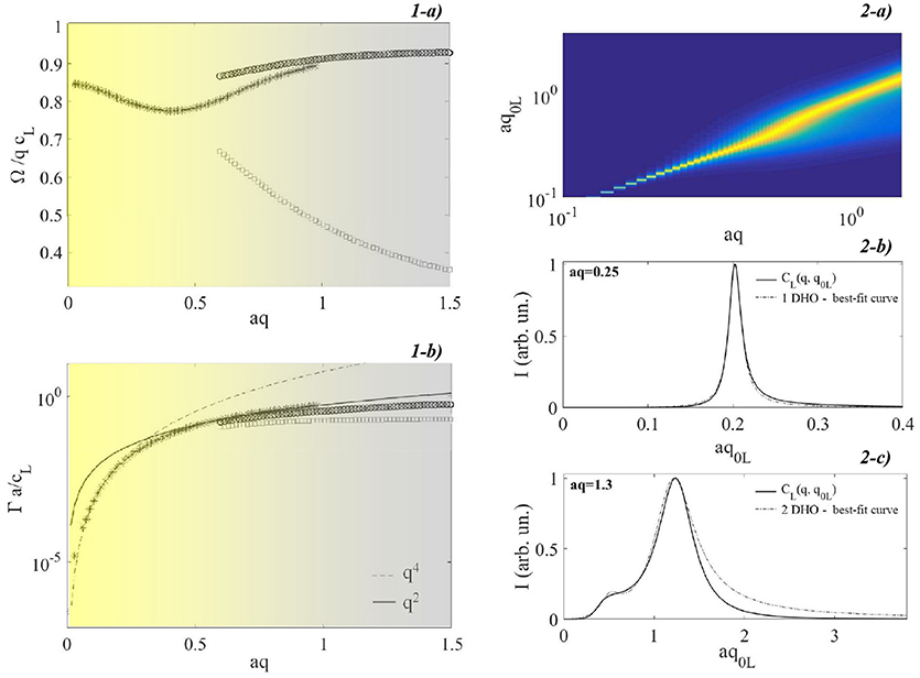
Figure 7. Features of the longitudinal acoustic dynamics obtained by exploiting the GBA both in the Rayleigh region, aq < < 1 and in the wavevectors region aq~1 where the mixing of polarizations shows up. (1-a). Adimensional phase velocity Ω/qc_L as a function of aq. Stars represent outcomes from 1-DHO model fitting, circles and squares represent outcomes from 2-DHO model fitting related respectively to high- and low-frequency features. (1-b) Adimensional attenuation Γa/c_L as function of aq. The meaning of the symbols is the same of (1-a). Full black line and dashed line are guide to eye displaying respectively the q⁴ and q² trend. (2-a) Projection on the (aq, aq_0L) plane of the longitudinal currents. (2-b) Representative longitudinal current spectrum in the Rayleigh region (full black line). The dashed line shows the best-fit curve with a 1-DHO fitting model. (2-c) Representative longitudinal current spectrum in the wavevector region where the mixing of polarizations is clearly observable (full black line). The dashed line shows the best-fit curve with a 2-DHO fitting model.

4. Conclusion

By introducing corrective terms to the Born Approximation we obtained in an analytic form an expression for the self-energy related to the stochastic Helmholtz equation describing the acoustic dynamics in an elestically heterogeneous medium. In the frame of the perturbative series expansion of the Dyson equation the proposed approximation accounts in an approximate form up to the second order term, whereas the Born Approximation stops to the first order. The Feynman diagram technique permits to clarify which multiple scattering events are included in the Generalized Born Approximation. The case of a covariance function given by an exponential decay function is analysed in some detail. In such a case it was proved the validity of the proposed approximation in a domain of the (ω, q) plane of interest in most topologically disordered systems (e.g., glasses). It includes both the Rayleigh region and wavevectors region: aq~1, where it is expected the mixing of polarizations to get in. Furthermore, the validity of the Generalized Born Approximation is not restricted to q in a neighbor of $\frac{\omega }{c_i}$, where c_i is the phase velocity of the unperturbed medium for the i-th polarization, thus permitting to describe also features of the average Green's dyadic occurring at frequencies smaller or higher than c_iq, as it is the case for the mixing of polarizations. We finally verified that the proposed approximation permits to describe this phenomenon together with the Rayleigh anomalies.

Acoustic modes with mixed polarization have been observed by both IXS and INS as well as by MD simulations in several disordered systems. The phenomenon has never been related, however, to Rayleigh anomalies and quantitatively described as a phenomenon also originating from the disordered nature of the medium. The proposed approximation can permit to reach this goal and to trace the way toward a coherent and experimentally verifiable mathematical description of all the phenomena arising from the elastic heterogeneous structure of an amorphous solid.

Author Contributions

MI led research, produced the results, and wrote the paper. GR and SC discussed the results and revisited the paper.

Conflict of Interest Statement

The authors declare that the research was conducted in the absence of any commercial or financial relationships that could be construed as a potential conflict of interest.

Acknowledgments

The authors acknoweldge W. Schirmacher and G. Pastore for useful discussions.

Supplementary Material

The Supplementary Material for this article can be found online at: https://www.frontiersin.org/articles/10.3389/fphy.2018.00108/full#supplementary-material

References

1. Ferrante C, Pontecorvo E, Cerullo G, Chiasera A, Ruocco G, Schirmacher W, et al. Acoustic dynamics of network-forming glasses at mesoscopic wavelengths. Nat Commun. (2013) 4:1793. doi: 10.1038/ncomms2826

PubMed Abstract | CrossRef Full Text | Google Scholar

2. Monaco G, Giordano V. Breakdown of the Debye approximation for the acoustic modes with nanometric wavelengths in glasses. Proc Natl Acad Sci USA. (2009) 106:3659. doi: 10.1073/pnas.0808965106

PubMed Abstract | CrossRef Full Text | Google Scholar

3. Ruta B, Baldi G, Scarponi F, Fioretto D, Giordano VM, Monaco G. Acoustic excitations in glassy sorbitol and their relation with the fragility and the boson peak. J Chem Phys. (2012) 137:214502. doi: 10.1063/1.4768955

PubMed Abstract | CrossRef Full Text | Google Scholar

4. Monaco G, Mossa S. Anomalous properties of the acoustic excitations in glasses on the mesoscopic length scale. Proc Natl Acad Sci USA. (2009) 106:16907. doi: 10.1073/pnas.0903922106

PubMed Abstract | CrossRef Full Text | Google Scholar

5. Baldi G, Giordano VM, Monaco G, Ruta B. Sound Attenuation at Terahertz Frequencies and the Boson Peak of Vitreous Silica. Phys Rev Lett. (2010) 104:195501. doi: 10.1103/PhysRevLett.104.195501

PubMed Abstract | CrossRef Full Text | Google Scholar

6. Nakayama T. Boson peak and terahertz frequency dynamics of vitreous silica. Rep Prog Phys. (2002) 65:1195. doi: 10.1088/0034-4885/65/8/203

CrossRef Full Text | Google Scholar

7. Schirmacher W, Ruocco G, Scopigno T. Acoustic attenuation in glasses and its relation with the Boson peak. Phys Rev Lett. (2007) 98:025501. doi: 10.1103/PhysRevLett.98.025501

PubMed Abstract | CrossRef Full Text | Google Scholar

8. John S, Stephen MJ. Wave propagation and localization in a long-range correlated random potential. Phys Rev B. (1983) 28:6358. doi: 10.1103/PhysRevB.28.6358

CrossRef Full Text | Google Scholar

9. Schirmacher W, Tomaras C, Schimid B, Viliani G, Baldi G, Ruocco G, et al. Vibrational excitations in systems with correlated disorder. Phys Stat Sol (2008) 5:862–6. doi: 10.1002/pssc.200777584

CrossRef Full Text | Google Scholar

10. Maurer E, Schirmacher W. Local oscillators vs. elastic disorder: a comparison of two models for the boson peak. J Low Temp Phys. (2004) 137:453–70. doi: 10.1023/B:JOLT.0000049065.04709.3e

CrossRef Full Text | Google Scholar

11. Marruzzo A, Schirmacher W, Fratalocchi A, Ruocco G. Heterogeneous shear elasticity of glasses: the origin of the boson peak. Sci Rep. (2013) 3:1407. doi: 10.1038/srep01407

PubMed Abstract | CrossRef Full Text | Google Scholar

12. Matic A, Engberg D, Masciovecchio C, Borjesson L. Sound wave scattering in network glasses. Phys Rev Lett. (2001) 86:3803–6. doi: 10.1103/PhysRevLett.86.3803

PubMed Abstract | CrossRef Full Text | Google Scholar

13. Masciovecchio C, Mermet A, Ruocco G, Sette F. Experimental evidence of the acousticlike character of the high frequency excitations in glasses. Phys Rev Lett. (2000) 85:1266–9. doi: 10.1103/PhysRevLett.85.1266

PubMed Abstract | CrossRef Full Text | Google Scholar

14. Rufflé B, Parshin DA, Courtens E, Vacher R. Boson peak and its relation to acoustic attenuation in glasses. Phys Rev Lett. (2008) 100:015501. doi: 10.1103/PhysRevLett.100.015501

PubMed Abstract | CrossRef Full Text | Google Scholar

15. Ayrinhac S, Foret M, Devos A, Rufflé B, Courtens E, Vacher R. Subterahertz hypersound attenuation in silica glass studied via picosecond acoustics. Phys Rev B (2011) 83:014204. doi: 10.1103/PhysRevB.83.014204

CrossRef Full Text | Google Scholar

16. Ruzicka B, Scopigno T, Caponi S, Fontana A, Pilla O, Giura P, et al. Evidence of anomalous dispersion of the generalized sound velocity in glasses. Phys Rev B (2004) 69:100201. doi: 10.1103/PhysRevB.69.100201

CrossRef Full Text | Google Scholar

17. Scopigno T, Pontecorvo E, Leonardo RD, Krisch M, Monaco G, Ruocco G, et al. High-frequency transverse dynamics in glasses. J Phys Condens Matter. (2003) 15:S1269. doi: 10.1088/0953-8984/15/11/345

CrossRef Full Text | Google Scholar

18. Zanatta M, Fontana A, Orecchini A, Petrillo C, Sacchetti F. Inelastic neutron scattering investigation in glassy SiSe2: complex dynamics at the atomic scale. J Phys Chem Lett. (2013) 4:1143–7. doi: 10.1021/jz400232c

PubMed Abstract | CrossRef Full Text | Google Scholar

19. Violini N, Orecchini A, Paciaroni A, Petrillo C, Sacchetti F. Neutron scattering investigation of high-frequency dynamics in glassy glucose. Phys Rev B (2012) 85:134204. doi: 10.1103/PhysRevB.85.134204

CrossRef Full Text | Google Scholar

20. Bolmatov D, Zhernenkov M, Sharpnack L, Agra-Kooijman DM, Kumar S, Suvorov A, et al. Emergent optical phononic modes upon nanoscale mesogenic phase transitions. Nano Lett. (2017) 17:3870–6. doi: 10.1021/acs.nanolett.7b01324

PubMed Abstract | CrossRef Full Text | Google Scholar

21. Bencivenga F, Antonangeli D. Positive sound dispersion in vitreous GeO2 at high pressure. Phys Rev B (2014) 90:134310. doi: 10.1103/PhysRevB.90.134310

CrossRef Full Text | Google Scholar

22. Cimatoribus A, Saccani S, Bencivenga F, Gessini A, Izzo MG, Masciovecchio C. The mixed longitudinal-transverse nature of collective modes in water. J Phys. (2010) 12:053008. doi: 10.1088/1367-2630/12/5/053008

CrossRef Full Text | Google Scholar

23. Calvet M, Margerin L. Velocity and attenuation of scalar and elastic waves in random media: a spectral function approach. J Acoust Soc Am. (2012) 131:1843–62. doi: 10.1121/1.3682048

PubMed Abstract | CrossRef Full Text | Google Scholar

24. Sobczyk K. Stochastic Wave Propagation. Warszawa: Elsevier (1985).

Google Scholar

25. Rytov SM, Kravtsov YA. Principles of Statistical Radiophysics 4 - Wave Propagation Through Random Media. Berlin: Springer-Verlag (1989).

Google Scholar

26. Bourret RC. Stochastically perturbed fields, with applications to wave propagation in random media. Nuovo Cim. (1962) 26:1–31. doi: 10.1007/BF02754339

CrossRef Full Text | Google Scholar

27. Turner AJ, Anugonda P. Scattering of elastic waves in heterogeneous media with local isotropy. J Acoust Soc Am. (2001) 109:1787–95. doi: 10.1121/1.1367245

PubMed Abstract | CrossRef Full Text | Google Scholar

28. Tomaras C, Schmid B, Schirmacher W. Anharmonic elasticity theory for sound attenuation in disordered solids with fluctuating elastic constants. Phys Rev B (2010) 81:104206. doi: 10.1103/PhysRevB.81.104206

CrossRef Full Text | Google Scholar

29. Blaustein N. Theoretical aspects of wave propagation in random media based on quanty and statistical field theory. Prog Electromag Res. (2004) 47:135–91. doi: 10.2528/PIER03111702

CrossRef Full Text | Google Scholar

30. Apresyan LA, Kravtsov YA. Radiation Transfer. Statistical and Wave Aspects. Philadelphia, PA: Gordon and Breach Publishers (1996).

Google Scholar

31. Kraichnan RH. Dynamics of nonlinear stochastic systems. J Math Phy. (1961) 2:124.

Google Scholar

32. Soven P. Coherent-potential model of substitutional disordered alloys. Phys Rev. (1967) 156:809.

Google Scholar

33. Taylor DW. Vibrational properties of imperfect crystals with large defect concentrations. Phys Rev. (1967) 156:1017–29.

Google Scholar

34. Elliott RJ, Krumhansl JA, Leath PL. The theory and properties of randomly disordered crystals and related physical systems. Rev Mod Phys. (1974) 46:465–563.

Google Scholar

35. Sheng P. Introduction To Wave Scattering, Localization and Mesoscopic Phenomena. San Diego, CA: Academic Press (1995).

Google Scholar

36. Kohler S, Ruocco G, Schirmacher W. Coherent potential approximation for diffusion and wave propagation in topologically disordered systems. Phys Rev B (2013) 88:064203. doi: 10.1103/PhysRevB.88.064203

CrossRef Full Text | Google Scholar

37. Jin J, Li J, Liu Y, Li XQ, Yan Y. Improved master equation approach to quantum transport: from born to self-consistent born approximation. J Chem Phys. (2014) 140:244111. doi: 10.1063/1.4884390

PubMed Abstract | CrossRef Full Text | Google Scholar

38. Li Z, Tong N, Zheng X, Hou D, Wei J, J Hu YY. Hierarchical Liouville-space approach for accurate and universal characterization of quantum impurity systems. Phys Rev Lett. (2012) 109:266403. doi: 10.1103/PhysRevLett.109.266403

PubMed Abstract | CrossRef Full Text | Google Scholar

39. Esposito M, Galperin M. Self-consistent quantum master equation approach to molecular transport. J Phys Chem C (2010) 114:20362–69. doi: 10.1021/jp103369s

CrossRef Full Text | Google Scholar

40. Ignatchenko VA, Polukhin DS. Development of a self-consistent approximation. J Phys A Math Theor. (2016) 49:095004. doi: 10.1088/1751-8113/49/9/095004

CrossRef Full Text | Google Scholar

41. Izzo MG, Wehinger B, Ruocco G, Matic A, Masciovecchio C, Gessini A, et al. Rayleigh anomalies and disorder-induced mixing of polarizations in amorphous solids. arXiv:170510338v2 [Prepint]. (2017).

Google Scholar

42. Zuniga M, Kong JA, Tsang L. Depolarization effects in the active remote sensing of random media. J Appl Phys. (1980) 51:2315–25.

Google Scholar

43. Lee JK, Kong JA. Active microwave remote sensing of an anisotropic random medium layer. IEEE Trans Geosci Remote Sensing GE (1985) 23:910–23.

Google Scholar

44. Jackson JD. Classical Electrodynamics. New York, NY: John Wiley and Sons (1962).

Google Scholar

45. Dirac PAM. The Principles of Quantum Mechanics. Oxford: Oxford University Press (1981).

Google Scholar

46. Torquato S. Exact conditions on physically realizable correlation functions of random media. J Chem Phys. (1999) 111:8832.

Google Scholar

47. Plemelj J. Riemannsche funktionenscharen mit gegebener monodromiegruppe. Monat Math Phys. (1908) 19:205.

Google Scholar

48. Fox C. A generalization of the Cauchy principal value. Can J Math. (1957) 9:110–7.

Google Scholar

49. Galapon EA. The Cauchy principal value and the Hadamard finite part integral as values of absolutely convergent integrals. J Math Phys. (2016) 57:033502. doi: 10.1063/1.4943300

CrossRef Full Text | Google Scholar

50. Quian T, Zhong T. Transformation formula of higher order integrals. J Austral Math Soc. (2000) 68:155–64. doi: 10.1017/S1446788700001919

CrossRef Full Text | Google Scholar

51. Kolmogorov AN, Fomin SV. Elements of the Theory of Functions and Functional Analysis. Rochester, NY: Graylock Press (1957).

52. Bolmatov D, Soloviov D, Zav'yalov D, Sharpnack L, Agra-Kooijman DM, Kumar S, et al. Anomalous nanoscale optoacoustic phonon mixing in nematic mesogens. J Phys Chem Lett. (2018) 9:2546–553.

PubMed Abstract | Google Scholar

53. Sampoli M, Ruocco G, Sette F. Mixing of longitudinal and transverse dynamics in liquid water. Phys Rev Lett. (1997) 79:1678.

Google Scholar

54. Bryk T, Ruocco G, Scopigno T, Seitsonen AP. Pressure-induced emergence of unusually high-frequency transverse excitations in a liquid alkali metal: evidence of two types of collective excitations contributing to the transverse dynamics at high pressures. J Chem Phys. (2015) 143:104502. doi: 10.1063/1.4928976

PubMed Abstract | CrossRef Full Text | Google Scholar

55. Ribeiro MCC. High-frequency acoustic modes in an ionic liquid. J Chem Phys. (2013) 139:114505. doi: 10.1063/1.4821227

PubMed Abstract | CrossRef Full Text | Google Scholar

56. Bolmatov D, Zhernenkov M, Zav'yalov D, Cai YQ, Cunsolo A. Terasonic excitations in 2D gold nanoparticle arrays in a water matrix as revealed by atomistic simulations. J Phys Chem C (2016) 120:19896–903. doi: 10.1021/acs.jpcc.6b08250

CrossRef Full Text | Google Scholar