Point-Particle Catalysis

1. Introduction

It is often the case that physically interesting situations involve a hierarchy of characteristic scales. For instance, solar system dynamics involve a variety of length scales, such as the sizes of the stars and planets involved, as well as the sizes of the orbits. Exploiting such a hierarchy by means of judicious Taylor expansions can greatly simplify otherwise very difficult problems, frequently even providing a handle on seemingly intractable problems. In the realm of quantum field theory, this insight has led to the development of the highly successful effective field theories, which can reduce the complexity of quantum field theories by restricting to parameter subspaces in which an appropriate Taylor expansion can be used to put the theory into a simpler form.

Usually, effective field theories exploit the hierarchy between interaction energies and the masses of some heavy particles to remove those heavy particles from the theory altogether (the quintessential example being Fermi's theory of the Weak interaction, which removes the heavy W and Z bosons) [1–4]. However, it is often the case that one's interest lies in a sector of the theory that still contains one or two of the heavy particles. For instance, in an atom, a heavy nucleus is present, but for most purposes there is no need to go about computing loops of nucleus-anti-nucleus pairs. Instead, higher energy nuclear dynamics are seen as finite nuclear-size effects. For this reason, an EFT has recently been explored that describes the remnant heavy particles in position-space to exploit the hierarchy of energy scales in a more intuitive expansion in kR, where k is the (small) momentum of the light particle and R is the length-scale of the nuclear structure [5–7]. This is accomplished in a simple way; the usual effective action is supplemented by a “point-particle” action that involves all possible couplings of the light particle to the worldline of the remnant heavy (point-like) particle (consistent with the symmetries of the low-energy theory). This type of “point-particle” EFT (PPEFT) is conceptually the next best thing to a Fermi type of EFT. While the nuclear dynamics cannot be removed altogether, they are significantly simplified.

The practicality of a PPEFT is two-fold: first it easily permits parameterizing physical quantities in terms of small nuclear properties, since the PPEFT expansion is directly in powers of kR. Second, that parameterization is completely general, and inherently includes all possible interactions, including any potential new physics. Some obvious examples that have been explored are cross-sections and bound-state energies of electrons in terms of nuclear charge radii [7, 8]. In this work, we ask the question: how do the small nuclear properties enter into physical quantities when there are multiple channels of interaction with the point-particle? (We ask this with mind toward eventually describing nuclear transfer reactions, and possibly baryon-monopole reactions which are known to suffer from questions of self-adjointedness of the Hamiltonian similar to those we address in this article [9, 10]).

To answer this question, we consider a simple toy model of two bulk Schrödinger (complex) fields coupled to the same point particle. The most general couplings to the point-particle's worldline y^μ(τ) are easily generalized from the single particle species (SP) examples explored in Burgess et al. [5] to the multi-particle (MP) case.

$\begin{array}{lll}\hfill S_b^{(\text{SP})}& =& -{\displaystyle \int }d\tau \sqrt{-{\dot{y}}^2}\left[M+h{\Psi }^{*}\Psi +\dots \right]\to \\ \hfill S_b^{(\text{MP})}& =& -{\displaystyle \int }d\tau \sqrt{-{\dot{y}}^2}\left[M+{\Psi }_i^{*}{h}_{ij}{\Psi }_j+\dots \right],& (1.1)\end{array}$

where Ψ, Ψ_i are bulk (complex) scalars, and the flavor index runs over 1 and 2. h_ij is a matrix of coupling constants that generalizes the single-particle coupling h, and the integral is over the proper time τ of the point-particle (${\dot{y}}^{\mathrm{\mu }}:=\frac{d{y}^{\mu }}{d\tau }$ is the point-particle's 4-velocity). Away from the point-particle, the action is just the usual Schrödinger action for (now) two scalars,

$\begin{array}{lll}{S}_B^{(\text{MP})}\hfill & =\hfill & {\displaystyle \sum _{i=1}^2{\displaystyle \int d^4}}x\{\frac{i}{2}\left({\Psi }_i^{*}{\partial }_t{\Psi }_i-{\Psi }_i{\partial }_t{\Psi }_i^{*}\right)\hfill \\ \hfill & \hfill & -\frac{1}{2m_i}|\nabla {\Psi }_i{|}^2-V(r)|{\Psi }_i{|}^2\}.\hfill & (1.2)\end{array}$

[V(r) is some bulk potential that may be sourced by the point-particle. In the main text we take it to be an inverse-square potential, since such a potential is highly singular and known to drive interesting behavior in a PPEFT [5]. For the moment it suffices to drop the potential]. If the bulk action (1.2) diagonalizes the momentum it need not diagonalize the brane action (1.1), and it is possible the off-diagonal elements of h (the matrix of h_ij) can source flavor-violating interactions.

In the center-of-mass reference frame (in the limit of infinite point-particle mass¹), the action (1.1) acts as a boundary condition at the origin for the modes of the Ψ_i fields. However, in general those diverge, and so the action has to be regulated at some finite radius ϵ. The couplings h must then be renormalized to keep physical quantities independent of the regulator, and it turns out that the (low-energy s-wave) cross-section for flavor violation is directly related to an invariant (ϵ₃) of the RG-flow of the off-diagonal h₁₂:

$\begin{array}{ll}{\sigma }_s^{(1\to 2)}=4\pi \frac{k_2}{k_1}{ϵ}_3^2,& (1.3)\end{array}$

where k₁ and k₂ are the incoming and outgoing momenta, respectively. For Schrödinger particles, the factor $k_2/k_1=\sqrt{m_2/m_1}$ is a constant. However, the same formula holds for spinless relativistic particles, and the ratio $k_2/k_1=\sqrt{(k_1^2+m_1^2-m_2^2)/k_1^2}$ leads to different qualitative behaviors of the low-energy cross-section depending on how k₁ relates to the mass gap $m_1^2-m_2^2$. If the mass gap is positive, and $k_1^2\ll m_1^2-m_2^2$, then the cross-section exhibits a 1/k₁ enhancement. Both the dependence on ϵ₃ and on k₁ may prove to be useful in a more complicated calculation, such as in mesic transfer reactions π⁰ + p → π⁺ + n (where the neutron and proton are in a nucleus), or possible flavor changing reactions involving new physics, such as μ⁻ + N → e⁻ + N [11, 12].

The channels of interaction with the point-particle do not have to be different bulk species, however. If, for example, the nucleus carried two accessible energy states, say E_↑ = M + Δ/2 and E_↓ = M − Δ/2 (where Δ ≪ M is some small excitation energy), then two channels of interaction could be a single bulk particle interacting with each of the nuclear energy eigenstates. In this case the “flavor-violating” cross section is again (1.3), where now k₁ and k₂ are the incoming and outgoing single-particle momenta, and $k_2/k_1=k_{\text{out}}/k_{\text{in}}=\sqrt{(k_{\text{in}}^2\pm 2m\Delta )/k_{\text{in}}^2}$ with the ± corresponding to the bulk particle impinging on a nucleus in the ground state (−) or the excited state (+), and where m is the mass of the single bulk species (recall we work in the non-recoil limit). On its own, this description is enough for any simple reaction ψ + N → ψ + N^*, where an incident non-relativistic particle just knocks a nucleus into a long-lived slightly energized state. Together, the two-species and two-nuclear state models form the building blocks for exploring more complicated processes, such as nuclear transfer reaction, where an incident particle exchanges some constituent particles with a nucleus, and the final state both violates flavor of the bulk species and changes the state of the source nucleus.

Finally, we can also look toward simpler models instead. One may imagine for instance only being interested in tracking one of the bulk-species, say particle 1 (perhaps an apparatus can only detect particles of flavor 1). In that case, the flavor-violating cross-section appears as an absorptive interaction when restricting to the particle 1 subspace of the theory. In this way, our toy model can be seen as a particular unitary completion of a model with a single particle subject to a non-self-adjoint Hamiltonian, as studied in Plestid et al. [13] and frequently used in the form of nuclear optical models [14, 15].

The rest of this paper is organized as follows. First, we briefly recall the salient details of a simple PPEFT for a single bulk species. Then in section 3, we establish the action and classical solutions to a point-particle EFT involving two bulk species, followed by section 4 in which we solve the boundary conditions of the system, and determine how all of the point-particle couplings run. All of this comes together in section 5 where we compute how the point-particle properties relate to physical cross-sections, including the cross-section for flavor-violation. In section 6 we connect the multi-bulk species story to a single particle coupled to a two-state nucleus. Finally, we wrap up in section 7 by restricting to a single-particle subsector of the multi-species model, and realizing the equivalence to the absorptive model of Plestid et al. [13].

2. Point-Particle EFT for a Single Bulk Species

We review the point-particle effective field theory for a single Schrödinger particle in an inverse-square potential, first described in Burgess et al. [5].

In the point-particle effective field theory approach, we exploit the hierarchy of length-scales between the characteristic wavelength of some low-energy particle of mass m (for concreteness, call this some scalar electron) and the scale of some small, almost point-like particle of mass M ≫ m it interacts with (similarly, we will call this a nucleus). For example, in atomic systems, this would be the ratio R/a₀ between the size R of a nucleus and the Bohr radius a₀ of the atom. For scattering, the small parameter is more directly kR, with k the wavenumber of the incident particle. The way we exploit this hierarchy is to recall that the low energy dynamics of the heavy particle are well approximated by ordinary quantum mechanics, so we imagine only first-quantizing the nucleus. In that case the fully second-quantized electron only couples to the 1-dimensional world-line of the heavy particle. This amounts to writing the action for the electron S = S_B + S_b in terms of the usual bulk dynamics²

$\begin{array}{ll}{S}_B={\displaystyle \int }{d}^{4}x\left\{\frac{i}{2}\left({\Psi }^{*}{\partial }_t\Psi -\Psi {\partial }_t{\Psi }^{*}\right)-\frac{1}{2m}|\nabla \Psi {|}^2-V(r)|\Psi {|}^2\right\}& (2.1)\end{array}$

as well as a boundary term consisting of interactions between the electron and the nuclear worldline,

$\begin{array}{ll}{S}_b=-{\displaystyle \int }d\tau \sqrt{-{\dot{y}}^2}\left(M+h|\Psi (y){|}^2+\dots \right).& (2.2)\end{array}$

In (2.1), V(r) may be some potential sourced by the point-particle, and the dots represent terms of higher powers in kR. In what follows, we choose $V(r)=\frac{g}{r^2}$. On its own, the excessive singularity of the inverse-square potential leads to ambiguities regarding the boundary condition at the origin [16]. Considerations of the self-adjointness of the Hamiltonian are often used to help resolve this difficulty, in particular by means of self-adjoint extensions [17–23]. A PPEFT however provides a natural solution to this problem by tying the near-source boundary condition unambiguously to the high-energy physics of the point particle, which may or may not lead to a self-adjoint Hamiltonian for the light degrees of freedom (for an example where probability for the bulk field is lost see [13], and the discussion in chapter 7, below). For a single bulk species this was considered in detail in Burgess et al. [5], and in particular it was shown that the inverse-square potential leads to a non-trivial renormalization of the point-particle coupling h. We briefly recall the results of that calculation below, and in the next section we will ask whether or not similar behavior is seen in the flavor-changing coupling.

Now through (2.2), there are couplings on the world-line y^μ(τ) of the nucleus (parameterized by its proper time τ, so that ${\dot{y}}^{\mathrm{\mu }}:=\frac{d{y}^{\mu }}{d\tau }$ is the 4-velocity of the nucleus). The first term $\sqrt{-{\dot{y}}^2}M$ can be recognized as the usual action for a point-particle [24], while the second term is the lowest-order (in powers of length) coupling between the electron and the nucleus, with the dots representing interactions of higher order in kR. For a spherically symmetric nucleus, the coupling h is a constant.

For simplicity, and to emphasize the value of the point-particle interactions, we work in the limit of infinite nuclear mass, where y^μ = (t, 0, 0, 0) is the center-of-mass frame, and τ = t. This amounts to neglecting nuclear recoil, but that can be included by explicitly tracking the dynamics of y^μ(τ). Requiring the action to remain stationary with respect to variations of Ψ^* that vanish on the boundary yields the usual Schrödinger equation in the bulk

$\begin{array}{ll}\left(i{\partial }_t+\frac{{\nabla }^2}{2m}-\frac{g}{r^2}\right)\Psi =0,& (2.3)\end{array}$

while including variations on the boundary leads to the boundary condition

$\begin{array}{ll}{\displaystyle \underset{ϵ\to 0}{lim}}4\pi {ϵ}^2{\partial }_{ϵ}{\Psi }_{\ell }={\displaystyle \underset{ϵ\to 0}{lim}}2mh{\Psi }_{\ell }(ϵ),& (2.4)\end{array}$

which defines ∂_ϵ : = ∂_r|_ϵ, Ψ_ℓ as the ℓ^th eigenfunction of angular momentum. However, it is typically the case that one cannot carry out the limit in (2.4)—indeed, in our effective theory, ϵ → 0 is the UV regime we do not claim to understand anyway. The solution to this problem is to replace the point-particle action (2.2) with a boundary action defined on the surface of a ball ${{B}}_{ϵ}$ of radius ϵ centered at the world-line of the point-particle (see Appendix A of [5]). In the center of mass frame of reference, this has the form:

$\begin{array}{ll}{{S}}_{{B}}=-\frac{1}{4\pi }{\displaystyle {\int }_{\partial {{B}}_{ϵ}}}{d}^2\Omega \left(M+{\displaystyle \sum _{\ell }}{h}_{\ell }|{\text{Ψ}}_{\ell }(ϵ){|}^2\right)& (2.5)\end{array}$

and yields the revised boundary condition

$\begin{array}{ll}4\pi {ϵ}^2{\partial }_{ϵ}{\Psi }_{\ell }=2m{h}_{\ell }{\Psi }_{\ell }(ϵ).& (2.6)\end{array}$

Here, h has been replaced by a different coupling h_ℓ to each angular momentum mode of the bulk particle (for more on why this is the case, see [13]). With the limit now gone, the fictitious scale ϵ appears explicitly in the boundary condition for the bulk field, and so runs the risk of appearing in physical quantities. The way around this is to observe that h_ℓ is not itself a physical quantity, and so must be renormalized with ϵ such that all physical quantities in the boundary condition (2.6) remain ϵ-independent. We explicitly compute this running next.

The bulk equations (2.3) (now defined only outside ${{B}}_{ϵ}$) are solved by

$\begin{array}{ll}\Psi =e^{-iEt}(C_{+}{\psi }_{+}+C_{-}{\psi }_{-})Y_{\ell ,m},& (2.7)\end{array}$

where E is the electron energy, Y_{ℓ, m} are the usual spherical harmonics, and the mode functions are

$\begin{array}{ll}{\psi }_{\pm }(\rho ):={\rho }^{\frac{1}{2}(-1\pm \zeta )}{e}^{-\rho /2}{M}\left[\frac{1}{2}(1\pm \zeta ),1\pm \zeta ;\rho \right]& (2.8)\end{array}$

which defines k² : = 2mE, ρ : = 2ikr, and $\zeta :=\sqrt{{(2\ell +1)}^2-8mg}$. For simplicity, in this paper we will restrict to the case mg ≤ 1/8 so that ζ is always real. Taking the small kϵ limit of (2.8), the boundary condition determines the renormalization-group flow of the coupling h_ℓ through

$\begin{array}{ll}\widehat{\lambda }=\frac{1-\frac{C_{-}}{C_{+}}{(2ikϵ)}^{-\zeta }}{1+\frac{C_{-}}{C_{+}}{(2ikϵ)}^{-\zeta }}=\frac{1+{(ϵ/{ϵ}_{\star })}^{-\zeta }}{1-{(ϵ/{ϵ}_{\star })}^{-\zeta }},& (2.9)\end{array}$

where $\widehat{\lambda }:=\frac{1}{\zeta }(mh/\pi ϵ+1)$ (we drop the subscript ℓ for convenience), $y:=\text{sgn}(|\widehat{\lambda }|-1)$ defines a renormalization-group trajectory, and ϵ_⋆ is an RG-invariant length scale, both determined by the physical quantity

$\begin{array}{ll}\frac{C_{-}}{C_{+}}=-y{(2ik{ϵ}_{\star })}^{\zeta }.& (2.10)\end{array}$

Physical quantities like scattering cross-sections and bound-state energies are directly related to the ratio C₋/C₊, and so through (2.10) directly to the quantity ϵ_⋆, which is fundamentally a property of the source. The usefulness of the inverse-square potential lies in how it can force non-trivial RG behavior upon the point-particle coupling. For example, the running (2.9) has an “infrared” fixed point of +1 when ϵ/ϵ_⋆ → ∞, which corresponds to ϵ_⋆ → 0. For the s-wave in the absence of an inverse-square potential, ζ(ℓ = 0) = 1 and this would be equivalent to vanishing point-particle coupling, but if the strength of the inverse-square potential g ≠ 0, then the fixed point is driven away from a vanishing point-particle coupling.

In the next section, we generalize all of this to a bulk system composed of multiple species of particles (though for concreteness, we specialize to two species). We see how most of the above follows through identically, but the presence of boundary terms that mix flavors adds a new degree of complexity to the problem, introducing a new point-particle coupling which runs differently from (2.9) and opening the door to flavor-changing reactions.

3. Multi-Species Action and Bulk Field Equations

The simplest extension of the basic point-particle action (2.2) to multiple particles is a non-diagonal quadratic one:

$\begin{array}{ll}{S}_b^{(\text{MP})}=-{\displaystyle \int }d\tau \sqrt{-{\dot{y}}^2}\left[M+{\Psi }_i^{*}{h}_{ij}{\Psi }_j+\dots \right]& (3.1)\end{array}$

where now there are N complex scalar Schroödinger fields Ψ_i, and summation over the species index is implied. The bulk action is taken to diagonalize the momentum operator, so flavor mixing only happens at the point particle, and the bulk action is simply N copies of (2.1):

$\begin{array}{ll}{S}_B^{(\text{MP})}& ={\displaystyle \sum _{i=1}^N}{\displaystyle \int }{d}^{4}x\{\frac{i}{2}\left({\Psi }_i^{*}{\partial }_t{\Psi }_i-{\Psi }_i{\partial }_t{\Psi }_i^{*}\right)\\ & -\frac{1}{2m_i}|\nabla {\Psi }_i{|}^2-V(r)|{\Psi }_i{|}^2\}.& (3.2)\end{array}$

For concreteness, we will work with only N = 2 species of particles. Our interest is in single particle states, so we restrict to the single-particle sector, for which the Hilbert space is ${H}=ℂ\oplus {{H}}_1\oplus {{H}}_2$ (where ${{H}}_i$ is the Hilbert space for particle i). On this space, the Schrödinger operator $i{\partial }_t+\frac{{\nabla }^2}{2m_i}-\frac{g}{r^2}$ is diagonal. Writing the total wavefunction $\Psi =\left(\begin{array}{l}{\Psi }_1\\ {\Psi }_2\end{array}\right)$, the equations of motion read

$\begin{array}{ll}\left[\begin{array}{cc}i{\partial }_t+\frac{{\nabla }^2}{2m_1}-\frac{g}{r^2}& 0\\ 0& i{\partial }_t+\frac{{\nabla }^2}{2m_2}-\frac{g}{r^2}\end{array}\right]\left[\begin{array}{c}{\Psi }_1\\ {\Psi }_2\end{array}\right]=0.& (3.3)\end{array}$

The time-dependence is easily solved using separation-of-variables: $\text{Ψ}=e^{-iEt}\left(\begin{array}{c}{\psi }_1\\ {\psi }_2\end{array}\right)$. Then we find

$\begin{array}{ll}\left[\begin{array}{cc}{k}_1^2+{\nabla }^2-\frac{g}{r^2}& 0\\ 0& k_2^2+{\nabla }^2-\frac{g}{r^2}\end{array}\right]\left[\begin{array}{c}{\psi }_1\\ {\psi }_2\end{array}\right]=0,& (3.4)\end{array}$

which defines the wavenumbers $k_i:=\sqrt{2m_{i}E}$ (real for continuum states and imaginary for bound states).

Away from the origin, (3.4) is solved exactly as in the single-species problem, and a natural choice of basis for the solutions is

$\begin{array}{ll}{B}=\left\{\left(\begin{array}{c}{\psi }_1\\ 0\end{array}\right),\left(\begin{array}{c}0\\ {\psi }_2\end{array}\right)\right\},& (3.5)\end{array}$

where

$\begin{array}{ll}{\psi }_i=\left(C_{i+}{\psi }_{+}({\ell }_i;2i{k}_{i}r)+C_{i-}{\psi }_{-}({\ell }_i;2k_{i}r)\right)Y_{{\ell }_i{m}_i}.& (3.6)\end{array}$

and

$\begin{array}{ll}{\psi }_{\pm }(\ell ;\rho ):={\rho }^{\frac{1}{2}(-1\pm {\zeta }_i)}{e}^{-\rho /2}{M}\left[\frac{1}{2}(1\pm {\zeta }_i),1\pm {\zeta }_i;\rho \right]& (3.7)\end{array}$

with ρ: = 2ikr, and ${\zeta }_i:=\sqrt{{(2\ell +1)}^2-8m_{i}g}$, and Y_{ℓi, mi} the usual spherical harmonics, as in the single-particle example.

The constants C_i± are solved by considering the boundary conditions in the problem, typically finiteness at large- and small-r, but for scattering problems the large-r BC is specific to the setup (since it depends on the presence or otherwise of incident particles). In a PPEFT, the small-r boundary condition is derived from the boundary action, which we describe next.

4. Boundary Conditions

In analogy with the single-particle system, we determine the small-r boundary condition by varying the point-particle action (3.1) directly [including the boundary terms in the variation of the bulk action (3.2)]. The resulting small-r boundary conditions are a simple generalization of (2.6):

$\begin{array}{ll}4\pi {ϵ}^2{\partial }_{ϵ}\Psi =2\text{mh}\Psi (ϵ),& (4.1)\end{array}$

again using $\text{Ψ}=e^{-iEt}\left(\begin{array}{c}{\psi }_1\\ {\psi }_2\end{array}\right)$ and as in section 2, we define ∂_ϵ: = ∂_r|_ϵ (and we drop the angular momentum label on h as above). Here m and h are the mass and point-particle coupling matrices (respectively), so that in components,

$\begin{array}{ll}4\pi {ϵ}^2{\partial }_{ϵ}{\psi }_1-2m_1{h}_{11}{\psi }_1(ϵ)-2m_1{h}_{12}{\psi }_2(ϵ)=0\text{\hspace{1em} and}& (\mathrm{4.2a})\end{array}$

$\begin{array}{ll}4\pi {ϵ}^2{\partial }_{ϵ}{\psi }_2-2m_2{h}_{22}{\psi }_2(ϵ)-2m_2{h}_{21}{\psi }_1(ϵ)=0.& (\mathrm{4.2b})\end{array}$

Notice that the explicit ϵ-dependence of (4.2) again indicates that the point-particle couplings h_ij must be renormalized with ϵ whenever Ψ or ∂_ϵΨ diverge for small argument, in order for the boundary condition to be compatible with the bulk equations of motion.

The boundary condition then serves two distinct purposes: (i) solving for the integration constants in Ψ tells us how they (and correspondingly physical quantities) depend on the point-source physics, and (ii) isolating for the couplings h_ij then tells us how exactly each coupling flows with ϵ to ensure the physical integration constants do not. Clearly though, with four possible degrees of freedom in h and four integration constants in Ψ, the two equations in (4.2) are insufficient by themselves. In the next sections we invoke physical arguments to resolve this predicament, and separately tackle both problems (i) and (ii).

4.1. Solving for Integration Constants

The most obvious place to look for additional constraints is at another boundary. In spherical coordinates, this amounts to looking at the asymptotic behavior of Ψ as r → ∞. However, the asymptotic behavior of the system is not unique, and is a very situation-dependent property. Since our interest in this paper is in catalysis of flavor violation, it is most pertinent to study scattering states.

First, focus on scattering Ψ₁ → Ψ_j. In this case, asymptotically we need (see Appendix A.2 for a review of multi-species scattering) ${\psi }_1(r\to \infty )\to e^{i{k}_{1}z}+f_{11}(\theta ,\psi )\frac{e^{i{k}_{1}r}}{k_{1}r}$ as usual, and now also ${\psi }_2(r\to \infty )\to f_{12}(\theta ,\psi )\frac{e^{i{k}_{2}r}}{k_{2}r}$. Notice that both boundary conditions and the equations of motion are linear in Ψ, so we may divide through by one integration constant. For incident particle 1, we will choose to divide through by C₁₊, and we will define

$\begin{array}{ll}{C}_{11}:=\frac{C_{1-}}{C_{1+}},\text{\hspace{1em}and\hspace{1em}}{C}_{12}:=\frac{C_{2-}}{C_{1+}}(1\to X\text{ scattering}),& (4.3)\end{array}$

and eliminating the infalling wave in ψ₂ fixes C₂₊ = RC₂₋ with

$\begin{array}{ll}R:=-\frac{\Gamma (1-\zeta /2)}{\Gamma (1+\zeta /2)}{2}^{-2\zeta }{e}^{-i\pi \zeta }& (4.4)\end{array}$

As we will see in the section 5, C₁₁ and C₁₂ are directly related to the physical cross-sections for Ψ₁ → Ψ₁ and Ψ₁ → Ψ₂ scattering.

Using the definitions (4.3) and (4.4) in the small-r boundary condition (4.2) yields

$\begin{array}{l}4\pi {ϵ}^2{\partial }_{ϵ}({\psi }_{1+}+C_{11}{\psi }_{1-})-h_{11}({\psi }_{1+}+C_{11}{\psi }_{1-})\\ -h_{12}{C}_{12}(R{\psi }_{2+}+{\psi }_{2-})=0\text{ and}& (\mathrm{4.5a})\end{array}$

$\begin{array}{lll}4\pi {ϵ}^2{C}_{12}{\partial }_{ϵ}(R{\psi }_{2+}+{\psi }_{2-})& -& h_{22}{C}_{12}(R{\psi }_{2+}+{\psi }_{2-})\\ & & -h_{21}({\psi }_{1+}+C_{11}{\psi }_{1-})& =0,& (\mathrm{4.5b})\end{array}$

Finally, in terms of integration constants the boundary condition (4.5) is now a system of two equations for two unknowns, so using the small-r forms of the bulk modes (3.7),

$\begin{array}{ll}& {\psi }_{\pm }(\ell ;ϵ)\approx {(2ikϵ)}^{\frac{1}{2}(-1\pm \zeta )}\Rightarrow \\ \frac{\partial }{\partial r}{|}_{ϵ}& {\psi }_{\pm }(\ell ;\rho )\approx ik(-1\pm \zeta ){(2ikϵ)}^{\frac{1}{2}(-3\pm \zeta )},& (4.6)\end{array}$

it is found (see Appendix B for details of the calculation) that the integration constants for this system are related to the source physics through

$\begin{array}{lll}\hfill C_{11}& =& -{(2i{k}_1ϵ)}^{{\zeta }_1}\frac{{\hat{{N}}}_1}{\hat{{D}}}\text{\hspace{1em} and}\\ \hfill C_{12}& =& {(2i{k}_1ϵ)}^{{\zeta }_1/2}{(2i{k}_2ϵ)}^{{\zeta }_2/2}\sqrt{\frac{m_2{k}_2{\zeta }_1}{m_1{k}_1{\zeta }_2}}\frac{{\widehat{\lambda }}_{21}}{\hat{{D}}},\end{array}$

where

$\begin{array}{ll}\hfill {\hat{{N}}}_1:& =4{\hat{\lambda }}_{12}{\hat{\lambda }}_{21}-\left[{\hat{\lambda }}_{11}-1\right]\left[{\hat{\lambda }}_{22}+1\right],\text{ and}\\ \hfill \hat{{D}}:& =4{\hat{\lambda }}_{12}{\hat{\lambda }}_{21}-\left[{\hat{\lambda }}_{11}+1\right]\left[{\hat{\lambda }}_{22}+1\right],& (4.7)\end{array}$

and the following convenient re-definitions have been made:

$\begin{array}{ll}\begin{array}{cc}{\hat{\lambda }}_{11}:=\frac{1}{{\zeta }_1}\left(\frac{m_1{h}_{11}}{\pi ϵ}+1\right),\hfill & {\hat{\lambda }}_{22}:=\frac{1}{{\zeta }_2}\left(\frac{m_2{h}_{22}}{\pi ϵ}+1\right),\text{ and},\hfill \end{array}\hfill & (4.8)\end{array}$

$\begin{array}{lll}{\hat{\lambda }}_{12}:=\frac{h_{12}\sqrt{m_1{m}_2}}{2\pi ϵ\sqrt{{\zeta }_1{\zeta }_2}},\hfill & {\hat{\lambda }}_{21}:=\frac{h_{21}\sqrt{m_1{m}_2}}{2\pi ϵ\sqrt{{\zeta }_1{\zeta }_2}}.\hfill & (4.9)\end{array}$

Of course, the choice to make particle 1 the incident particle was not forced upon us, and with foresight to the next sections, we also compute the quantities involved in scattering Ψ₂ → Ψ_i. Fortunately, this is exactly the 1 ↔ 2 inversion of the 1 → X scattering above, so we can immediately write:

$\begin{array}{lll}4\pi {ϵ}^2{C}_{12}{\partial }_{ϵ}(R{\psi }_{2+}+{\psi }_{2-})& -& h_{22}{C}_{12}(R{\psi }_{2+}+{\psi }_{2-})\hfill \\ & -& h_{21}({\psi }_{1+}+C_{11}{\psi }_{1-})=0\text{ and}\hfill & (\mathrm{4.10a})\end{array}$

$\begin{array}{lll}4\pi {ϵ}^2{\partial }_{ϵ}({\psi }_{1+}+C_{11}{\psi }_{1-})& -& h_{11}({\psi }_{1+}+C_{11}{\psi }_{1-})\\ & -& h_{12}{C}_{12}(R{\psi }_{2+}+{\psi }_{2-})=0,& (\mathrm{4.10b})\end{array}$

where as above we have defined

$\begin{array}{ll}{C}_{22}:=\frac{C_{2-}}{C_{2+}},\text{\hspace{1em}and\hspace{1em}}{C}_{21}:=\frac{C_{1-}}{C_{2+}}(2\to X\text{ scattering}),& (4.11)\end{array}$

now with C₁₊ = RC₁₋. Solving for the integration constants similarly yields

$\begin{array}{lll}\hfill C_{22}& =& -{(2i{k}_2ϵ)}^{{\zeta }_2}\frac{{\hat{{N}}}_2}{\hat{{D}}}\text{\hspace{1em} and}\\ \hfill C_{21}& =& {(2i{k}_1ϵ)}^{{\zeta }_1/2}{(2i{k}_2ϵ)}^{{\zeta }_2/2}\sqrt{\frac{m_1{k}_1{\zeta }_2}{m_2{k}_2{\zeta }_1}}\frac{{\widehat{\lambda }}_{12}}{\hat{{D}}},& (4.12)\end{array}$

where now

$\begin{array}{ll}{\hat{{N}}}_2:=4{\hat{\lambda }}_{12}{\hat{\lambda }}_{21}-\left[{\hat{\lambda }}_{11}+1\right]\left[{\hat{\lambda }}_{22}-1\right].& (4.13)\end{array}$

It is important to note that the C_ij integration constants are fundamentally different, as they are determined by different asymptotic boundary conditions and correspond to different physics. In section 5 we will see exactly how they relate to the physical cross-sections, but having defined them all separately is already important at the level of renormalizing the point-particle couplings, which we do next.

4.2. Renormalization-Group Flows and Invariants

Next we move on to teasing out of the boundary condition (4.2) exactly how the couplings h_ij must be renormalized with ϵ to keep physical quantities independent of the regulator. One way to do so would be to differentiate (4.7) and (4.11) with respect to ϵ while holding the (physical) integration constants fixed, and solve the resulting differential equations. This approach turns out to be very difficult however, since the equations are highly coupled and tough to disentangle. Notice however that it is important to have knowledge of both 1 → X and 2 → X scattering to solve for all the elements of h. This is not a coincidence. A unitary system requires a real action, which is enforced by the condition that h is Hermitian. At the same time, a unitary S-matrix for an N-species system has N² real degrees of freedom, which is the same dimension as an N × N Hermitian matrix. Consequently, connecting the point-particle couplings to physical quantities requires knowledge of the entire S-matrix, and so in our case must involve both 1 → X scattering and 2 → X scattering. Lastly, one final simplification can be made by observing that the phase of h₁₂ can be removed by a field redefinition, so for the special case of a two-species system we only have to deal with a real matrix of point-particle couplings.

The easiest approach to solving for the flows of the couplings h_ij is to go back to the boundary conditions (4.5) and (4.9) for both 1 → X and 2 → X systems and solve directly for the individual elements of h. This inversion is done in detail in Appendix C, and using the small-r form (4.6), the point-particle couplings must take the following forms as functions of the regulator ϵ.

$\begin{array}{ll}{\hat{\lambda }}_{11}=\frac{(1-C_{11}{\left(2i{k}_1ϵ\right)}^{-{\zeta }_1})(1+C_{22}{\left(2i{k}_2ϵ\right)}^{-{\zeta }_2})+C_{21}{C}_{12}{\left(2i{k}_1ϵ\right)}^{-{\zeta }_1}{\left(2i{k}_2ϵ\right)}^{-{\zeta }_2}}{(1+C_{11}{\left(2i{k}_1ϵ\right)}^{-{\zeta }_1})(1+C_{22}{\left(2i{k}_2ϵ\right)}^{-{\zeta }_2})-C_{21}{C}_{12}{\left(2i{k}_1ϵ\right)}^{-{\zeta }_1}{\left(2i{k}_2ϵ\right)}^{-{\zeta }_2}},& (\mathrm{4.14a})\end{array}$

$\begin{array}{lll}{\hat{\lambda }}_{12}& =\sqrt{\frac{m_2{\zeta }_1}{m_1{\zeta }_2}}\frac{C_{21}{\left(\frac{k_1}{k_2}\right)}^{-1/2}{(2i{k}_1ϵ)}^{-{\zeta }_1/2}{(2i{k}_2ϵ)}^{-{\zeta }_2/2}}{(1+C_{11}{(2i{k}_1ϵ)}^{-{\zeta }_1})(1+C_{22}{(2i{k}_2ϵ)}^{-{\zeta }_2})-C_{21}{C}_{12}{(2i{k}_1ϵ)}^{-{\zeta }_1}{(2i{k}_2ϵ)}^{-{\zeta }_2}},& (\mathrm{4.14b})\end{array}$

$\begin{array}{lll}{\hat{\lambda }}_{21}& =\sqrt{\frac{m_1{\zeta }_2}{m_2{\zeta }_1}}\frac{C_{12}{\left(\frac{k_2}{k_1}\right)}^{-1/2}{(2i{k}_1ϵ)}^{-{\zeta }_1/2}{(2i{k}_2ϵ)}^{-{\zeta }_2/2}}{(1+C_{11}{(2i{k}_1ϵ)}^{-{\zeta }_1})(1+C_{22}{(2i{k}_2ϵ)}^{-{\zeta }_2})-C_{21}{C}_{12}{(2i{k}_1ϵ)}^{-{\zeta }_1}{(2i{k}_2ϵ)}^{-{\zeta }_2}},& (\mathrm{4.14c})\end{array}$

$\begin{array}{lll}{\hat{\lambda }}_{22}& =\frac{(1+C_{11}{(2i{k}_1ϵ)}^{-{\zeta }_1})(1-C_{22}{(2i{k}_2ϵ)}^{-{\zeta }_2})+C_{21}{C}_{12}{(2i{k}_1ϵ)}^{-{\zeta }_1}{(2i{k}_2ϵ)}^{-{\zeta }_2}}{(1+C_{11}{(2i{k}_1ϵ)}^{-{\zeta }_1})(1+C_{22}{(2i{k}_2ϵ)}^{-{\zeta }_2})-C_{21}{C}_{12}{(2i{k}_1ϵ)}^{-{\zeta }_1}{(2i{k}_2ϵ)}^{-{\zeta }_2}},& (\mathrm{4.14d})\end{array}$

using the definitions (4.9).

Equations (4.13) (together with (4.7), (4.11), (2.10), and past work [8]) suggests the integration constants can each be characterized by a unique RG-invariant length-scale. To see how this works, define the scales ϵ₁, ϵ₂, and ϵ₃ by the following relations:

$\begin{array}{ll}\hfill \begin{array}{cccc}\hfill & \hfill C_{11}& =\hfill & -y_1{(2i{k}_1{ϵ}_1)}^{{\zeta }_1},C_{22}=-y_2{(2i{k}_2{ϵ}_2)}^{{\zeta }_2},\hfill \\ \hfill \text{and }& \hfill C_{12}& =\hfill & \frac{m_2{k}_2{\zeta }_1}{m_1{k}_1{\zeta }_2}{C}_{21}=y_3\sqrt{\frac{m_2{k}_2{\zeta }_1}{m_1{k}_1{\zeta }_2}}{(2i{k}_1{ϵ}_3)}^{{\zeta }_1/2}{(2i{k}_2{ϵ}_3)}^{{\zeta }_2/2},\hfill \end{array}& (4.15)\end{array}$

where y_i = ±1 defines a particular class of flow. In terms of these scales, the running equations are significantly simpler:

$\begin{array}{ll}{\hat{\lambda }}_{11}=\frac{\left(1+y_1{(ϵ/{ϵ}_1)}^{-{\zeta }_1}\right)\left(1-y_2{(ϵ/{ϵ}_2)}^{-{\zeta }_2}\right)+{(ϵ/{ϵ}_3)}^{-({\zeta }_1+{\zeta }_2)}}{\left(1-y_1{(ϵ/{ϵ}_1)}^{-{\zeta }_1}\right)\left(1-y_2{(ϵ/{ϵ}_2)}^{-{\zeta }_2}\right)-{(ϵ/{ϵ}_3)}^{-({\zeta }_1+{\zeta }_2)}},& (\mathrm{4.16a})\end{array}$

$\begin{array}{lll}{\hat{\lambda }}_{12}& =& {\hat{\lambda }}_{21}\\ & =& \frac{y_3{(ϵ/{ϵ}_3)}^{-({\zeta }_1+{\zeta }_2)/2}}{\left(1-y_1{(ϵ/{ϵ}_1)}^{-{\zeta }_1}\right)\left(1-y_2{(ϵ/{ϵ}_2)}^{-{\zeta }_2}\right)-{(ϵ/{ϵ}_3)}^{-({\zeta }_1+{\zeta }_2)}},& (\mathrm{4.16b})\end{array}$

$\begin{array}{ll}{\hat{\lambda }}_{22}=\frac{\left(1-y_1{(ϵ/{ϵ}_1)}^{-{\zeta }_1}\right)\left(1+y_2{(ϵ/{ϵ}_2)}^{-{\zeta }_1}\right)+{(ϵ/{ϵ}_3)}^{-({\zeta }_1+{\zeta }_2)}}{\left(1-y_1{(ϵ/{ϵ}_1)}^{-{\zeta }_1}\right)\left(1-y_2{(ϵ/{ϵ}_2)}^{-{\zeta }_2}\right)-{(ϵ/{ϵ}_3)}^{-({\zeta }_1+{\zeta }_2)}},& (\mathrm{4.16c})\end{array}$

An example of ${\hat{\lambda }}_{11}$ and ${\hat{\lambda }}_{22}$ is plotted in Figure 1, and an example of ${\hat{\lambda }}_{12}$ is plotted in Figure 2. All the couplings flow to fixed points in the ultraviolet (ϵ/ϵ_i → 0) and the infrared (ϵ/ϵ_i → ∞). The diagonal couplings ${\hat{\lambda }}_{11}$ and ${\hat{\lambda }}_{22}$ both flow to −1 in the UV and +1 in the IR, exactly as the single-particle flow does, while the off-diagonal ${\hat{\lambda }}_{12}$ flows to vanishing coupling in both the cases. This says something reasonable: the system is perfectly content to live in a world where there is no species mixing, regardless of the existence of the inverse-square potential. However, if the species do mix, then the strength of that mixing depends on the scale it is measured at, with the flow given by (4.15b).

FIGURE 1

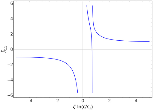
Figure 1. Plot of ${\hat{\lambda }}_{11}$ vs ζ ln(ϵ/ϵ₁) for ζ₁ = ζ₂, y₁ = y₂ = +1, and ${({ϵ}_2/{ϵ}_1)}^{\zeta }=2$ and ${({ϵ}_3/{ϵ}_1)}^{\zeta }=0.02$. The fascinating second pole arises in certain limits of the ratio of ϵ₁ to ϵ₂ and ϵ₃. In the limit ϵ₃ → 0, this reduces to the classic single-particle RG.

FIGURE 2

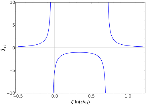
Figure 2. Plot of ${\hat{\lambda }}_{12}$ vs ζ ln(ϵ/ϵ₁) for ζ₁ = ζ₂, y₁ = y₂ = y₃ = +1, and ${({ϵ}_2/{ϵ}_1)}^{\zeta }=2$ and ${({ϵ}_3/{ϵ}_1)}^{\zeta }=0.02$.

Interestingly, all three flows share a common denominator, which can always be factorized. When ζ₁ = ζ₂ = : ζ, the zeroes of the denominator lie at

$\begin{array}{ll}{ϵ}_a^{\zeta }=\frac{1}{2}\left(y_2{ϵ}_2^{\zeta }+y_1{ϵ}_1^{\zeta }\pm \sqrt{{\left(y_1{ϵ}_1^{\zeta }-y_2{ϵ}_2^{\zeta }\right)}^2+4{ϵ}_3^{2\zeta }}\right),& (4.17)\end{array}$

so there is at least one asymptote in all the flows as long as $y_2{ϵ}_2^{\zeta }+y_1{ϵ}_1^{\zeta }>0$. Indeed, the only regime where there is no asymptote is where $-(y_2{ϵ}_2^{\zeta }+y_1{ϵ}_1^{\zeta })>\sqrt{{(y_1{ϵ}_1^{\zeta }-y_2{ϵ}_2^{\zeta })}^2+4{ϵ}_3^{2\zeta }}>0$.

The practicality of this framework lies in how the point-particle couplings [and in particular their RG-invariants (4.14)] inform physical quantities, like scattering cross-sections, and we investigate this next.

5. Scattering and Catalysis of Flavor Violation

To see how the nuclear properties enter into macroscopic quantities, and in particular how the point-particle can induce a violation of bulk flavor-conservation, we proceed to compute the elements of the scattering matrix. In particular, it will be shown that the low-energy s-wave “elastic” (Ψ_i → Ψ_i) scattering is as usual independent of incoming momentum, and ϵ_i plays the role of the scattering length. Meanwhile, the flavor-violating “inelastic” cross-section is uniquely characterized by ϵ₃, which can be thought of as an effective scattering length for flavor violation. Moreover, the inelastic cross-section goes as k_out/k_in. This ratio is a constant for Schrödinger particles, but for Klein-Gordon fields (such as is appropriate for, say, incident pions) the ratio has a dependence on the incoming momentum, and that dependence takes on a variety of qualitatively different forms determined by the size of $k_{\text{in}}^2/|m_1^2-m_2^2|$. Of particular interest is the case where the incoming particle's mass is greater than the outgoing particle's mass, and the incoming particle's momentum is small compared to the mass gap, in which case the flavor-violating cross-section is catalyzed, and goes as 1/k_in (although such a setup would certainly be hard to realize in practice).

Following the Appendix A.2, we need to identify the scattering matrix elements $S_{ij}^{(\ell )}$ in terms of C_ij.

5.1. Elastic Scattering (ψ_i → ψ_i)

First consider elastic scattering of ψ₁. This is the case where the measured particle is the same as the incoming particle, so the asymptotic form of ψ₁ contains an incoming plane wave and an outgoing spherical wave:

$\begin{array}{ll}{\psi }_1^{\text{Ans}}(r\to \infty )\to {C}\left(e^{i{k}_{1}z}+f_{11}(\theta ,\psi )\frac{e^{i{k}_{1}r}}{r}\right).& (5.1)\end{array}$

Starting from the general form (3.6) for particle 1,

$\begin{array}{ll}{\psi }_1=(C_{1+}{\psi }_{1+}+C_{1-}{\psi }_{1-})Y_{{\ell }_1,m_1},& (5.2)\end{array}$

the large-r limit is (taking the asymptotic limit of the confluent hypergeometric function)

$\begin{array}{ll}{\psi }_1(r\to \infty )\to A_{\ell }\frac{e^{i(k_{1}r-\ell \pi /2)}}{2i{k}_{1}r}+B_{\ell }\frac{e^{-i(k_{1}r-\ell \pi /2)}}{2i{k}_{1}r},& (5.3)\end{array}$

where

$\begin{array}{ll}\begin{array}{ccc}\hfill A_{\ell }& =\hfill & \left[\Gamma \left(1+\frac{1}{2}{\zeta }_1\right)2^{{\zeta }_1}{C}_{1+}+\Gamma \left(1-\frac{1}{2}{\zeta }_1\right)2^{-{\zeta }_1}{C}_{1-}\right]\frac{e^{i\pi \ell /2}}{\sqrt{\pi }},\text{\hspace{1em}and}\hfill \\ \hfill B_{\ell }& =\hfill & \left[\Gamma \left(1+\frac{1}{2}{\zeta }_1\right)2^{{\zeta }_1}{C}_{1+}+\Gamma \left(1-\frac{1}{2}{\zeta }_1\right)2^{-{\zeta }_1}{e}^{-i\pi {\zeta }_1}{C}_{1-}\right]\frac{e^{i(1+{\zeta }_1-\ell )\pi /2}}{\sqrt{\pi }}.\hfill \end{array}\hfill & (5.4)\end{array}$

Matching to the asymptotic form (5.1), allows us to identify (see 12.1) the overall normalization

$\begin{array}{lll}{C}& =& \frac{{(-1)}^{\ell +1}}{2\pi \sqrt{(2\ell +1)}}[\Gamma \left(1+\frac{1}{2}{\zeta }_1\right)2^{{\zeta }_1}{C}_{1+}\\ & & +\Gamma \left(1-\frac{1}{2}{\zeta }_1\right)2^{-{\zeta }_1}{e}^{-i\pi {\zeta }_1}{C}_{1-}]e^{i(1+{\zeta }_1)\pi /2},& (5.5)\end{array}$

and the scattering matrix element

$\begin{array}{ll}& S_{11}^{(\ell )}=-\frac{A_{\ell }}{B_{\ell }}\\ =& \frac{\left[\Gamma (1+{\zeta }_1/2)+\Gamma (1-{\zeta }_1/2)2^{-2{\zeta }_1}{C}_{11}\right]}{\left[\Gamma (1+{\zeta }_1/2)+\Gamma (1-{\zeta }_1/2)2^{-2{\zeta }_1}{e}^{-i\pi {\zeta }_1}{C}_{11}\right]}{e}^{i(2\ell +1-{\zeta }_1)\pi /2}.& (5.6)\end{array}$

Our interest is in the regime where k_iϵ is small, so the s-wave is the dominant contribution to the cross-section. In the s-wave, ${\zeta }_1={\zeta }_{1s}:=\sqrt{1-8m_{1}g}$, and the cross-section is (A.9), exactly as in Burgess et al. [6]:

$\begin{array}{ll}{\sigma }_s^{(1\to 1)}=\frac{\pi }{k_1^2}|S_{11}^{(0)}{|}^2=\frac{\pi }{k_1^2}|\frac{1-{A}{e}^{i\pi {\zeta }_{1s}/2}}{1-{A}{e}^{-i\pi {\zeta }_{1s}/2}}{|}^2& (5.7)\end{array}$

where

$\begin{array}{ll}{A}:=e^{-i\pi {\zeta }_1/2}{2}^{-2{\zeta }_1}{C}_{11}\frac{\Gamma \left[1-\frac{1}{2}{\zeta }_1\right]}{\Gamma \left[1+\frac{1}{2}{\zeta }_1\right]}=y_1{\left(\frac{k_1{ϵ}_1}{2}\right)}^{{\zeta }_1}\frac{\Gamma \left[1-\frac{1}{2}{\zeta }_1\right]}{\Gamma \left[1+\frac{1}{2}{\zeta }_1\right]}.& (5.8)\end{array}$

[The second equality uses (4.14) to exchange the integration constants for the RG-invariant ϵ₁]. Of particular note is when there is no inverse-square potential, in which case ζ_1s = 1 and the cross-section reduces to

$\begin{array}{ll}{\sigma }_s^{(1\to 1)}=4\pi {ϵ}_1^2(g=0),& (5.9)\end{array}$

which can be identified as the cross-section for scattering from a 3D δ-function potential (see for example [25] where our ϵ₁ corresponds to their $g/\sqrt{\pi }$). Elastic scattering for the second species ψ₂ → ψ₂ follows exactly the same procedure and is trivially the 1 ↔ 2 inversion of (5.7) and (5.8).

$\begin{array}{ll}{\sigma }_s^{(2\to 2)}=4\pi {ϵ}_2^2(g=0).& (5.10)\end{array}$

5.2. Flavor-Violating Scattering (ψ_i → ψ_j, i ≠ j)

So much for the ordinary scattering. Finally we compute the flavor-violating ψ₁ → ψ₂ cross-section, and see the point-particle catalysis in action. This time, there is no incoming flux of the particle to be measured, so the large-r ansatz is simply:

$\begin{array}{ll}{\psi }_2^{\text{Ans}}(r\to \infty )\to {C}{f}_2(\theta ,\psi )\frac{e^{i{k}_{2}r}}{r}.& (5.11)\end{array}$

where we have scaled out the same normalization factor ${C}$, for convenience. The asymptotic form of the general solution for ψ₂ is exactly (5.3) subject to 1 ↔ 2, so we can immediately observe the following. First, as was used in deriving the boundary conditions in section 4, B_ℓ = 0 so that C₂₊ = RC₂₋, where as above

$\begin{array}{ll}R:=-\frac{\Gamma (1-\zeta /2)}{\Gamma (1+\zeta /2)}{2}^{-2\zeta }{e}^{-i\pi \zeta }.& (5.12)\end{array}$

Following Appendix A.2, this time we identify the inelastic scattering element $S_{12}^{(\ell )}$ using (A.15)

$\begin{array}{lll}{S}_{12}^{(\ell )}& =& \frac{e^{-i\pi \ell /2}}{\sqrt{4\pi (2\ell +1)}}\frac{A_{\ell }}{{C}}=\frac{\Gamma \left(1-\frac{1}{2}{\zeta }_2\right)}{2\pi \sqrt{(2\ell +1)}}\frac{C_{2-}}{{C}}{2}^{-{\zeta }_2}(1-e^{-i\pi {\zeta }_2}),\\ & =& \frac{{(-1)}^{-\ell +1}}{2^{{\zeta }_1+{\zeta }_2-1}}\text{ sin }(\pi {\zeta }_2/2)e^{i\pi (\ell -{\zeta }_1-{\zeta }_2-1)/2}\frac{\Gamma \left(1-\frac{1}{2}{\zeta }_2\right)}{\Gamma \left(1+\frac{1}{2}{\zeta }_1\right)}\frac{C_{12}}{1-{A}{e}^{-i\pi {\zeta }_1/2}}.& (5.13)\end{array}$

where ${A}$ is defined in (5.8).

Again, our interest is in the small k_iϵ regime for which the s-wave dominates. We similarly define ${\zeta }_{2s}:=\sqrt{1-8m_{2}g}$. Then the low-energy cross-section is (A.16),

$\begin{array}{lll}{\sigma }_s^{(1\to 2)}& =& \frac{\pi }{k_1{k}_2}\frac{m_1}{m_2}|S_{12}^{(0)}{|}^2,\\ & =& \frac{4\pi }{2^{{\zeta }_1+{\zeta }_2}}\frac{k_1^{{\zeta }_1}{k}_2^{{\zeta }_2}}{k_1^2}\frac{{\zeta }_1}{{\zeta }_2}{\text{ sin}}^2(\pi {\zeta }_2/2)\frac{{ϵ}_3^{{\zeta }_1+{\zeta }_2}}{|1-{A}{e}^{-i\pi {\zeta }_1/2}{|}^2}{\left(\frac{\Gamma \left(1-\frac{1}{2}{\zeta }_2\right)}{\Gamma \left(1+\frac{1}{2}{\zeta }_1\right)}\right)}^2.& (5.14)\end{array}$

As in the elastic case, the reverse scattering ψ₂ → ψ₁ is a simple matter of exchanging 1 ↔ 2 in (5.14). In the absence of an inverse-square potential (ζ_is = 1), the cross-section (5.14) simplifies significantly.

$\begin{array}{ll}{\sigma }_s^{1\to 2}=4\pi \frac{k_2}{k_1}{ϵ}_3^2(g=0).& (5.15)\end{array}$

On its own, this is an interesting enough result. The flavor-violating cross-section is non-zero only when the point-particle has non-trivial flavor-violating properties, as are encoded in ϵ₃. This is also the statement that flavor-violation only occurs if h₁₂ ≠ 0, since it is always true—regardless of the presence of an inverse-square potential—that h₁₂ = 0 only when ϵ₃ = 0³.

A particularly interesting aspect of (5.15) is the factor of k₂/k₁. For Schrödinger particles, this is just a constant ($k_i=\sqrt{2m_{i}E}\Rightarrow k_2/k_1=\sqrt{m_2/m_2}$). In section 6, we treat a Schrödinger particle interacting with a multi-state nucleus, in which case the final and initial momenta do differ non-trivially, but even at the level of two bulk species, more interesting dynamics can be seen just by treating the particles as relativistic Klein-Gordon fields. For relativistic fields, the cross-section takes the same general form as (5.15), except the momenta are relativistic: $k_i=\sqrt{{\omega }^2-m_i^2}$, where ω is the energy of the system. Then ${\omega }^2=k_i^2+m_i^2$, so that

$\begin{array}{ll}\frac{k_2}{k_1}=\frac{\sqrt{k_1^2+\left(m_1^2-m_2^2\right)}}{k_1}.& (5.16)\end{array}$

The cross-section therefore exhibits different qualitative behavior depending on how the incoming momentum k₁ relates to the (squared) mass gap $m_1^2-m_2^2$. This can be broadly classified by 4 different regimes depending on the sign of $m_1^2-m_2^2$ and the size of the ratio $r:=k_1^2/|m_1^2-m_2^2|$.

First, if the mass gap is positive, the only question is to the size of the ratio r. If r ≪ 1, then ${\sigma }_s^{(1\to 2)}~k_1^{-1}$. This is the regime where the cross-section sees a low-energy enhancement similar to the well-known enhancement of absorptive cross-sections [26] (more on that in section 6). However, if r ≫ 1, then the cross-section is roughly independent of the incoming momentum altogether. The cross-over between these regimes is plotted in Figure 3. These are indeed reasonable behaviors. If m₁ > m₂, and the incoming momentum is small compared to the mass difference, then the transition is to a lighter particle traveling faster, which is intuitively a more favorable process—the heavier incident particle has access to a larger phase-space than the lighter incident particle. If the mass difference is small compared to the incoming momentum, then the benefit of transitioning to a particle with a smaller mass is minimal, so the process is no more favorable than no transition. If instead the mass gap is negative, then there is a new regime. If $k_1^2<m_2^2-m_1^2$ (so if r < 1) there is in fact no scattering. This is certainly reasonable—if the incident particle did not have enough energy to create the rest mass of the second particle, then it cannot scatter into that particle (this is the threshold behavior described by [27, section 144]). If r ≳ 1, the incident momentum is just enough to create the second particle $k_1^2=m_2^2-m_1^2+\delta$, then the cross-section goes as $\sqrt{\delta /(m_2^2-m_1^2)}$. Since $k_2^2=k_1^2+m_1^2-m_2^2=\delta \ll m_2^2$, this is also the statement that the cross-section goes as v₂, the (non-relativistic) speed of the final state particle. Finally, if r ≫ 1, the incident momentum greatly exceeds the mass gap and we again see the cross-section behave independently from k₁, as before. These momentum-dependences are plotted in Figure 4.

FIGURE 3

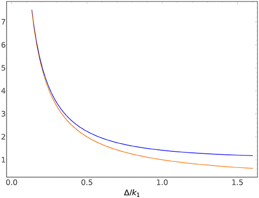
Figure 3. Plot of the cross-over behavior in the k dependence of the inelastic cross-section for a Klein-Gordon particle conversion in units of Δ/k₁, where $\Delta =\sqrt{m_1^2-m_2^2}$ and m₁ > m₂. The full function $\sqrt{1+{\Delta }^2/k_1^2}$ is plotted in blue, and the simple inelastic behavior Δ/k₁ is plotted in orange. Notice the overlap for small Δ/k₁, and the strong enhancement for large momenta.

FIGURE 4

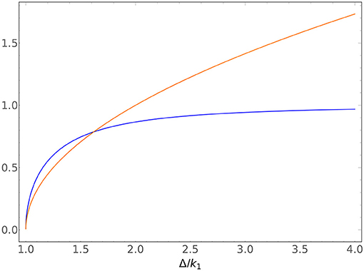
Figure 4. Plot of the cross-over behavior in the k dependence of the inelastic cross-section for a Klein-Gordon particle conversion in units of Δ/k₁, where $\Delta =\sqrt{m_1^2-m_2^2}$ and m₂ > m₁. The full function $\sqrt{1-{\Delta }^2/k_1^2}$ is plotted in blue, and the simple inelastic behavior $\sqrt{\Delta /k_1-1}$ is plotted in orange. Notice the threshold cutoff at Δ/k₁ = 1, as well as the approximate overlap for small Δ/k₁, and the strong suppression for large momenta.

6. Transfer Reactions and Nuclear Structure

In many cases, a reaction with a nucleus can change not only the incident particle, but also the nucleus. This can be the case even when scattering energies are low compared to the mass of the nucleus. For instance, the excitation energy of most real nuclei is on the order of MeV compared to their masses of order GeV [28]. A particularly interesting class of reactions that falls into this category is transfer reactions, where a composite particle (say a neutron) scatters off of a nucleus and exchanges a constituent particle (say a quark) with one of the valence nucleons, so that the outgoing particle is different (perhaps a proton) and so is the nucleus. While this work is not enough to describe a complete transfer reaction, we can make progress toward a complete description, and can at least describe the simpler process ψ + N → ψ + N^*, where N is some nucleus and N^* is a long-lived excited state of that nucleus. The key observation to make is that there is essentially no difference between a system spanned by {Ψ₁ ⊗ |N〉, Ψ₂ ⊗ |N〉} with |N〉 some nuclear state, and {Ψ ⊗ |N₁〉, Ψ ⊗ |N₂〉} where |N_i〉 are distinct nuclear states. The only complexity lies in describing the different nuclear states in a point-particle EFT language.

Here we will sketch out the simplest point-particle action that includes a two-state nucleus coupled to a single bulk field, but a more detailed treatment of a PPEFT for a point-particle with internal degrees of freedom will be available in Zalavái et al. (in preparation). In addition to the single-species action (2.2), introduce an auxiliary grassmann-valued field T_i that satisfies the commutation relations of the generators of 𝔰𝔲(2).

$\begin{array}{lll}{S}_b^{\text{2N}}& =& -{\displaystyle \int }d\tau \sqrt{-{\dot{y}}^2}(M+i{T}_i{\dot{T}}^i-i{ϵ}_{ijk}{\Delta }_i{T}_j{T}_k+h^{\prime }|\Psi (y(\tau )){|}^2\\ & & -{ϵ}_{ijk}{g}_i^{\prime }{T}_j{T}_k|\Psi (y(\tau )){|}^2).& (6.1)\end{array}$

Here, Δ_i and $g_i^{\prime }$ are 3-vector-valued parameters. For convenience, we work in the basis such that Δ_i = Δδ_i3. Furthermore, we collect the point-particle couplings involving Ψ as $W=W^{†}:=h^{\prime }-\frac{i}{2}{g}_i^{\prime }{T}_i$.

Upon quantization, the T_i can be identified with $\frac{i}{2}{\sigma }_i$, the generators of 𝔰𝔲(2), and since they only live on the point-particle's world-line, it is easy to see that they are associated with a two-level nuclear state. Varying the action with respect to y(τ) (and neglecting the subdominant contribution from the W interactions), the nuclear dispersion relation

$\begin{array}{ll}\langle N|{\widehat{p}}_N^2-M^2+\Delta {\sigma }_z|N\rangle =0,& (6.2)\end{array}$

(${\widehat{p}}_N$ is the nuclear 4-momentum operator) leads to distinct nuclear states |↑〉 with rest-frame energy E_↑ = M + Δ/2 and |↓〉 with rest-frame energy E_↓ = M − Δ/2.

The bulk action for the system is exactly the single-particle Schrödinger action (2.1), and so the solutions for Ψ are precisely (2.7) and (2.8). However, the boundary condition (2.6) becomes:

$\begin{array}{ll}\langle \uparrow \downarrow |4\pi {ϵ}^2{\partial }_{ϵ}\Psi |\Xi \rangle =\langle \uparrow \downarrow |W\Psi (ϵ)|\Xi \rangle ,& (6.3)\end{array}$

where |Ξ〉 is an appropriate Fock state, |↑↓〉 are the Fock states consisting of just the nucleus in the state with rest-frame energy E_↑↓, and Ψ is interpreted as an operator-valued field. Since energy can now be exchanged between the electron and the nucleus, the individual energies of the electron and the nucleus are no longer good quantum numbers, and a general single-electron Fock state must be a linear combination |Ξ〉 = |Ψ_↑〉|↑〉 + |Ψ_↓〉|↓〉, where |Ψ_↑↓〉 has energy ω_↑↓ satisfying ω_↑ + Δ/2 = ω_↓ − Δ/2. Then in terms of the mode-functions ${\text{Ψ}}_{\uparrow \downarrow }(x)=e^{-i{\omega }_{\uparrow \downarrow }}{\psi }_{\uparrow \downarrow }$ (satisfying Ψ|Ψ_↑↓〉 = Ψ_↑↓(x)|Ψ_↑↓〉), the boundary condition (6.3) is in components,

$\begin{array}{ll}\begin{array}{c}4\pi {ϵ}^2{\partial }_{ϵ}{\psi }_{\uparrow }-W_{\uparrow \uparrow }{\psi }_{\uparrow }(ϵ)-W_{\uparrow \downarrow }{\psi }_{\downarrow }(ϵ)=0\text{\hspace{1em} and}\hfill \\ 4\pi {ϵ}^2{\partial }_{ϵ}{\psi }_{\downarrow }-W_{\downarrow \downarrow }{\psi }_{\downarrow }(ϵ)-W_{\downarrow \uparrow }{\psi }_{\uparrow }(ϵ)=0,\hfill \end{array}\hfill & (6.4)\end{array}$

where we identified the T_i with $\frac{1}{2}{\sigma }_i$ so that $W=h^{\prime }{𝕀}_{2\times 2}+\frac{1}{4}{g}_i^{\prime }{\sigma }_i$. The boundary condition (6.4) is now exactly the boundary condition (4.2) with W ↔ h and ψ_↑↓ ↔ ϕ_{1, 2}.

Finally, defining E: = ω_↑ + Δ/2 = ω_↓ − Δ/2, we observe $k_{\uparrow }^2=2m{\omega }_{\uparrow }=2m(E-\Delta /2)$ and $k_{\downarrow }^2=2m{\omega }_{\downarrow }=2m(E+\Delta /2)$. Choosing ψ_↑ ↔ ψ₁ and ψ_↓ ↔ ψ₂, we may then identify k₁ = k_↑ and k₂ = k_↓. At this point, a complete analogy with the two-species system is established, and the results are tabulated into a dictionary relating the two in Table 1. A true transfer reaction is one for which the final state involves both a different species of bulk particle and an altered state of the nucleus, so evidently would be equivalent to a model of 4 bulk species coupled to a single-state point-particle. As it stands however, this system is sufficient to describe, say, the low-energy behavior of a neutron that knocks a nucleus into its first excited state.

TABLE 1

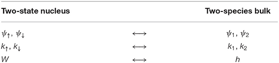
Table 1. The dictionary that maps quantities in a two-bulk-species theory to quantities in a theory of a single bulk-species coupled to a point-particle with two accessible internal degrees of freedom.

7. Single-Particle Subsector

In many cases it is overkill to track all of the possible final state products of a particular interaction. This is especially the case in nuclear physics, where a summation over many unobserved final states is the basis of the highly successful optical model [14, 15]. The price one pays for the convenience of ignoring certain states is the loss of unitarity, and such a non-unitary point-particle EFT was the subject of Plestid et al. [13]. Here we can provide a very simple explicit example of how this non-unitarity can emerge in a subsector of a larger unitary theory. We achieve this correspondence by matching physical quantities, in a procedure that is significantly simpler than e.g., tracing the partition function over the states involving Ψ₂ [29, 30].

From Plestid et al. [13], the key to a point-particle inducing a violation of unitarity is allowing the point-particle coupling to be complex (h from section 2). In that case, the running of the coupling is the same as (2.9), except now the constant $-y\to e^{i{\alpha }_{\star }}$ is complex. That is:

$\begin{array}{ll}{\widehat{\lambda }}_c=\frac{1-e^{i{\alpha }_{\star }}{(ϵ/{ϵ}_{\star })}^{-\zeta }}{1+e^{i{\alpha }_{\star }}{(ϵ/{ϵ}_{\star })}^{-\zeta }},& (7.1)\end{array}$

where ${\widehat{\lambda }}_c$ is the now complex coupling. Similarly, the integration constant is analogous to (2.10),

$\begin{array}{ll}\frac{C_{-}}{C_{+}}={(2ikϵ)}^{\zeta }\frac{1-{\widehat{\lambda }}_c}{1+{\widehat{\lambda }}_c}={(2ik{ϵ}_{\star })}^{\zeta }{e}^{i{\alpha }_{\star }}.& (7.2)\end{array}$

At this point, we essentially have everything we need. The ratio of integration constants $\frac{C_{-}}{C_{+}}$ is directly related to the physical quantities in the single-particle problem, so choosing to track either Ψ₁ or Ψ₂ tells us to equate (7.2) to C₁₁ or C₂₂ (respectively), and from that determine how the RG-invariants and couplings are related. The only obstruction at this point is that (4.14) would at face value suggest that α_⋆ = nπ and there is no absorptive scattering. The error here is that inelastic scattering is a sub-leading effect⁴, and to see it at the level of C₁₁, we would need to have computed that ratio of integration constants to sub-leading order in k_iϵ. This is not in itself a particularly challenging endeavor, and is done in the Appendix B. The result is that to sub-leading order, one finds (B.22) (choosing to track Ψ₁, tracking Ψ₂ follows trivially)

$\begin{array}{lll}{C}_{11}& =& -{(2i{k}_1ϵ)}^{{\zeta }_1}\frac{{\hat{{N}}}_1}{\hat{{D}}}\left(1-4R\frac{{\widehat{\lambda }}_{12}{\widehat{\lambda }}_{21}}{{\hat{{N}}}_1\hat{{D}}}{(2i{k}_2ϵ)}^{{\zeta }_2}\right)\\ & =& -y_1{(2i{k}_1{ϵ}_1)}^{{\zeta }_1}(1+i\delta {\alpha }_1).& (7.3)\end{array}$

From the last equality, we use that δα₁ ≪ 1 to define $e^{i{\alpha }_1}\approx -y_1(1+i\delta {\alpha }_1)$ such that α₁: = nπ + δα₁, with n an integer that satisfies $y_1:=-e^{in\pi }$. Since (7.3) is a perturbative expression, we may use the leading order (in k_iϵ) expressions for the couplings in δα₁, and simply evaluate them at ϵ = ϵ₁. An alternative but more tedious approach would be to substitute the second equality in (7.3) into ${\widehat{\lambda }}_{11}$ [taking the whole function to sub-leading order in k_iϵ as in (C.12)] and solve for δα₁ by demanding ${\widehat{\lambda }}_{11}$ remain real at sub-leading order, as it must. No matter the approach, the result is

$\begin{array}{ll}\delta {\alpha }_1=-{(2k_2{ϵ}_3)}^{{\zeta }_1}{\left(\frac{{ϵ}_3}{{ϵ}_1}\right)}^{{\zeta }_2}\frac{\left|R\right|}{y_1}\text{ sin}(\pi {\zeta }_2/2).& (7.4)\end{array}$

In this way, we have solved for the RG-invariant quantities (and so too the physical quantities) in the single-particle absorptive model in terms of the RG-invariants in the unitary two-species model simply by equating C₁₁ to C₋/C₊. In fact, we can do even better than that. We can determine how the coupling ${\widehat{\lambda }}_c$ relates to the various ${\hat{\lambda }}_{ij}$ couplings. To do so, we simply arrange for ${\hat{{N}}}_A/\hat{{D}}$ to take the form of $({\widehat{\lambda }}_c-1)/({\widehat{\lambda }}_c+1)$.

$\begin{array}{ll}\frac{{\hat{{N}}}_1}{\hat{{D}}}=\frac{4|{\hat{\lambda }}_{12}{|}^2-\left[{\hat{\lambda }}_{11}-1\right]\left[{\hat{\lambda }}_{22}+1\right]}{4|{\hat{\lambda }}_{12}{|}^2-\left[{\hat{\lambda }}_{11}+1\right]\left[{\hat{\lambda }}_{22}+1\right]}=\frac{\frac{{\hat{\lambda }}_{11}\left[{\hat{\lambda }}_{22}+1\right]-4|{\hat{\lambda }}_{12}{|}^2}{\left[{\hat{\lambda }}_{22}+1\right]}-1}{\frac{{\hat{\lambda }}_{11}\left[{\hat{\lambda }}_{22}+1\right]-4|{\hat{\lambda }}_{12}{|}^2}{\left[{\hat{\lambda }}_{22}+1\right]}+1}.& (7.5)\end{array}$

Evidently ${\widehat{\lambda }}_c={\hat{\lambda }}_{11}-4|{\hat{\lambda }}_{12}{|}^2/\left[{\hat{\lambda }}_{22}+1\right]$. A check on this is to directly compute the combination ${\hat{\lambda }}_{11}-4|{\hat{\lambda }}_{12}{|}^2/\left[{\hat{\lambda }}_{22}+1\right]$, in which case one finds it is exactly (7.1) with ϵ_⋆ and α_⋆ defined as above. This dictionary between these models is laid out in Table 2.

TABLE 2

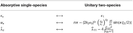
Table 2. The dictionary that maps quantities in a unitary two-species theory to quantities in a non-unitary single-species theory.

Data Availability Statement

All datasets generated for this study are included in the article/supplementary material.

Author Contributions

PH wrote most of the text and derived most of the results. CB provided significant guidance, corrected errors, helped with interpretations, and provided feedback on the manuscript.

Funding

This research was supported in part by funds from the Natural Sciences and Engineering Research Council (NSERC) of Canada. Research at the Perimeter Institute is supported in part by the Government of Canada through Industry Canada, and by the Province of Ontario through the Ministry of Research and Information (MRI).

Conflict of Interest

The authors declare that the research was conducted in the absence of any commercial or financial relationships that could be construed as a potential conflict of interest.

Acknowledgments

We thank László Zalavári, Daniel Ruiz, Markus Rummel, and Ryan Plestid for helpful discussions.

Footnotes

1. ^We neglect here recoil effects, though those can be included by tracking the dynamics of y^μ(τ).

2. ^We use a mostly plus metric, and work in units such that ℏ = c = 1.

3. ^As noted in section 4.2, this is in contrast to the behavior of h₁₁ and h₂₂, whose flows indicate that ϵ₁, ϵ₂ → 0 is only consistent with h₁₁, h₂₂ → 0 when there is no inverse-square potential.

4. ^The way to see this is through the catalysis cross-section (5.15). Absorptive scattering generically scales as a/k for some absorptive scattering length a. The derived cross-section (5.15) identifies a ~ (k₂ϵ₃)ϵ₃ and so is generically a subdominant effect in the point-particle EFT regime.

References

1. Burgess CP. An introduction to effective field theory. Annu Rev Nucl Part Sci. (2007) 57:329–62. doi: 10.1146/annurev.nucl.56.080805.140508

CrossRef Full Text | Google Scholar

2. Burgess CP, Moore GD. The Standard Model: A Primer. Cambridge: Cambridge University Press (2006).

Google Scholar

3. Weinberg S. The Quantum Theory of Fields. Vol. 1. Cambridge: Cambridge University Press (1995).

4. Weinberg S. The Quantum Theory of Fields. Vol. 2. Cambridge: Cambridge University Press (1996).

Google Scholar

5. Burgess CP, Hayman P, Williams M, Zalavári L. Point-particle effective field theory I: classical renormalization and the inverse-square potential. J High Energy Phys. (2017) 2017:106. doi: 10.1007/JHEP04(2017)106

CrossRef Full Text | Google Scholar

6. Burgess CP, Hayman P, Rummel M, Williams M, Zalavári L. Point-particle effective field theory II: relativistic effects and Coulomb/inverse-square competition. J High Energy Phys. (2017) 2017:72. doi: 10.1007/JHEP07(2017)072

CrossRef Full Text | Google Scholar

7. Burgess CP, Hayman P, Rummel M, Zalavári L. Point-particle effective field theory III: relativistic fermions and the Dirac equation. J High Energy Phys. (2017) 2017:7. doi: 10.1007/JHEP09(2017)007

CrossRef Full Text | Google Scholar

8. Burgess CP, Hayman P, Rummel M, Zalavri L. Reduced theoretical error for ⁴He⁺ spectroscopy. Phys Rev A. (2018) 98:052510. doi: 10.1103/PhysRevA.98.052510

CrossRef Full Text | Google Scholar

9. Kazama Y, Yang CN, Goldhaber AS. Scattering of a Dirac particle with charge Ze by a fixed magnetic monopole. Phys Rev D. (1977) 15:2287–99. doi: 10.1103/PhysRevD.15.2287

CrossRef Full Text | Google Scholar

10. D'Hoker E, Farhi E. The abelian monopole fermion system and its self-adjoint extensions as a limit of a non-abelian system. Phys Lett B. (1983) 127:360–4.

Google Scholar

11. Pezzullo G. The Mu2e experiment at Fermilab: a search for lepton flavor violation. Nucl Part Phys Proc. (2017) 285-86:3–7. doi: 10.1016/j.nuclphysbps.2017.03.002

CrossRef Full Text | Google Scholar

12. Bonventre R. Searching for muon to electron conversion: the Mu2e experiment at Fermilab. SciPost Phys Proc. (2019) 1:038. doi: 10.21468/SciPostPhysProc.1.038

CrossRef Full Text | Google Scholar

13. Plestid R, Burgess CP, O'Dell DHJ. Fall to the centre in atom traps and point-particle EFT for absorptive systems. J High Energy Phys. (2018) 2018:59. doi: 10.1007/JHEP08(2018)059

CrossRef Full Text | Google Scholar

14. Feshbach H. Nuclear reactions. In: Digital Encyclopedia of Applied Physics. American Cancer Society (2003). Available online at: https://onlinelibrary.wiley.com/doi/abs/10.1002/3527600434.eap277

Google Scholar

15. Dickhoff WH, Charity RJ. Recent developments for the optical model of nuclei. Prog Part Nucl Phys. (2019) 105:252–99. doi: 10.1016/j.ppnp.2018.11.002

CrossRef Full Text | Google Scholar

16. Essin AM, Griffiths DJ. Quantum mechanics of the 1/x2 potential. Am J Phys. (2006) 74:109–17. doi: 10.1119/1.2165248

CrossRef Full Text | Google Scholar

17. Capri AZ. Self-adjointness and spontaneously broken symmetry. Am J Phys. (1977) 45:823–25. doi: 10.1119/1.11055

CrossRef Full Text | Google Scholar

18. Dupré MJ, Goldstein JA, Levy M. The nearest self-adjoint operator. J Chem Phys. (1980) 72:780–1. doi: 10.1063/1.438923

CrossRef Full Text | Google Scholar

19. Bonneau G, Faraut J, Valent G. Self-adjoint extensions of operators and the teaching of quantum mechanics. Am J Phys. (2001) 69:322–31. doi: 10.1119/1.1328351

CrossRef Full Text | Google Scholar

20. Borg JL, Pulé JV. Pauli approximations to the self-adjoint extensions of the Aharonov-Bohm Hamiltonian. J Math Phys. (2003) 44:4385–410. doi: 10.1063/1.1601298

CrossRef Full Text | Google Scholar

21. Araujo VS, Coutinho FaB, Fernando Perez J. Operator domains and self-adjoint operators. Am J Phys. (2004) 72:203–13. doi: 10.1119/1.1624111

CrossRef Full Text | Google Scholar

22. Camblong HE, Epele LN, Fanchiotti H, García Canal CA, Ordónez CR. On the inequivalence of renormalization and self-adjoint extensions for quantum singular interactions. Phys Lett A. (2007) 364:458–64. doi: 10.1016/j.physleta.2006.12.041

CrossRef Full Text | Google Scholar

23. Fülöp T. Singular potentials in quantum mechanics and ambiguity in the self-adjoint hamiltonian. SIGMA Symmet Integrabil Geomet Methods Appl. (2007) 3:107. doi: 10.3842/SIGMA.2007.107

CrossRef Full Text

24. Lambert N. String theory 101. In: Baumgartl M, Brunner I, Haack M, editors. Strings and Fundamental Physics. Lecture Notes in Physics. Berlin; Heidelberg: Springer Berlin Heidelberg (2012). p. 1–48. Available online at: https://doi.org/10.1007/978-3-642-25947-0_1

Google Scholar

25. Jackiw R editor. Delta function potentials in two-dimensional and three-dimensional quantum mechanics. In: Diverse Topics in Theoretical and Mathematical Physics. Singapore: World Scientific (1991).

Google Scholar

26. Bethe HA. Theory of disintegration of nuclei by neutrons. Phys Rev. (1935) 47:747–59. doi: 10.1103/PhysRev.47.747

CrossRef Full Text | Google Scholar

27. Landau LD, Lifshitz EM. Chapter XVIII - Inelastic collisions. In: Landau LD, Lifshitz EM, editors. Quantum Mechanics, 3rd Edn. Pergamon (1977). p. 591–646. Available online at: http://www.sciencedirect.com/science/article/pii/B9780080209401500256

28. Audi G, Kondev FG, Wang M, Huang WJ, Naimi S. The NUBASE2016 evaluation of nuclear properties. Chin Phys C. (2017) 41:030001. doi: 10.1088/1674-1137/41/3/030001

CrossRef Full Text | Google Scholar

29. Feldman HA, Kamenshchik AY. Decoherence properties of scalar field perturbations. Class Quant Grav. (1991) 8:L65–71. doi: 10.1088/0264-9381/8/3/003

CrossRef Full Text | Google Scholar

30. Burgess CP, Holman R, Tasinato G, Williams M. EFT beyond the horizon: stochastic inflation and how primordial quantum fluctuations go classical. J High Energy Phys. (2015) 2015:90. doi: 10.1007/JHEP03(2015)090

CrossRef Full Text | Google Scholar

31. Landau LD, Lifshitz EM. Chapter XVII - Elastic Collisions In: Landau LD, Lifshitz EM, editors. Quantum Mechanics, 3rd Edn. Pergamon (1977). p. 502–90.

Google Scholar

Appendix

A. Multi-Particle Partial-Wave Scattering

Here we review the general framework of partial-wave scattering, including discussion of inelastic and multi-channel scattering.

A.1. Single Particle Elastic Scattering

We consider a spinless particle scattering off of a spinless, infinitely massive object at rest at the origin, through a spherically symmetric interaction V(r). As usual, we employ the ansatz that at large distances from the target, the wavefunction of the incident particle is the sum of a plane wave incident along the z-axis and a scattered spherical wave:

$\begin{array}{ll}{\psi }_{\infty }^{\text{Ans}}(r)\to C\left(e^{ikz}+f(\theta ,\varphi )\frac{e^{ikr}}{r}\right).& (\mathrm{A1})\end{array}$

The differential cross-section is the ratio of the flux of the scattered particles F_sc to the flux of the incoming particles F_in. With an incident beam of N particles, the incoming flux is $N{\text{j}}_{in}·{\text{e}}_z=N|{C}{|}^{2}k/m$, and the scattered flux is $N\left|{C}{|}^2\right|f(\theta ,\varphi ){|}^{2}k/m{r}^2$, so that and is given by

$\begin{array}{ll}\frac{d\sigma }{d\Omega }:=\frac{F_{sc}}{F_{in}}=\frac{1}{F_{in}}{j}_{sc}\cdot e_r{r}^2={\left|f(\theta )\right|}^2.& (\mathrm{A2})\end{array}$

And for a spherically symmetric scatterer, f(θ, ϕ) = f(θ).

At the same time, we consider solutions to the full Schrodinger equation

$\begin{array}{ll}\frac{1}{r^2}{\partial }_r\left(r^2{\partial }_r\psi (r)\right)-\left[\frac{\ell (\ell +1)}{r^2}+2mV(r)-k^2\right]\psi (r)=0,& (\mathrm{A3})\end{array}$

with k²: = 2mE, and the full wavefunction expanded in a series of spherical harmonics $\text{Ψ}(\overrightarrow{x},t)=e^{-iEt}\psi (r)Y_{\ell 0}$ (where we set m = 0 due to conservation of angular momentum). The asymptotic form of these radial functions is:

$\begin{array}{ll}{\psi }_{\infty }^{\text{Sch}}(r)\to A_{\ell }\frac{e^{i(kr-\ell \pi /2)}}{2ikr}+B_{\ell }\frac{e^{-i(kr-\ell \pi /2)}}{2ikr},& (\mathrm{A4})\end{array}$

Finding f(θ) now amounts to matching (A1) and (A4). This can be accomplished by writing the plane-wave e^ikz in terms of Legendre polynomials. The standard expansion is given as Landau and Lifshitz [31]

$\begin{array}{l}{e}^{ikz}={\displaystyle \sum _{\ell =0}^{\infty }(2\ell +1)}{i}^{\ell }{j}_{\ell }(kr)P_{\ell }(\cos (\theta ))\hfill \\ \to {\displaystyle \sum _{\ell =0}^{\infty }(2\ell +1)}{i}^{\ell }\frac{e^{i(kr-\ell \pi /2)}-e^{-i(kr-\ell \pi /2)}}{2ikr}{P}_{\ell }(\cos (\theta )).\hfill & (\mathrm{A5})\end{array}$

Choosing the Condon-Shortly phase convention, the spherical harmonics can be written $Y_{\ell }^0=\sqrt{(2\ell +1)/4\pi }{P}_{\ell }(\text{cos}(\theta ))$, so by computing the difference:

$\begin{array}{ll}{\psi }_{\infty }^{\text{Sch}}(r)-C{e}^{ikz}=Cf(\theta )\frac{e^{ikr}}{r},& (\mathrm{A6})\end{array}$

one finds first:

$\begin{array}{ll}{B}_{\ell }=-\sqrt{4\pi (2\ell +1)}{i}^{\ell }C,& (\mathrm{A7})\end{array}$

set by the fact that there can be no incoming wave in the scattered wavefunction. Finally, one finds

$\begin{array}{ll}f(\theta )=\frac{1}{2ik}{\displaystyle \sum _{\ell =0}^{\infty }(2\ell +1)}\left[S_{\ell }-1\right]P_{\ell }(\theta ),& (\mathrm{A8})\end{array}$

Where S_ℓ = −A_ℓ/B_ℓ is the scattering matrix element. When the scattering is elastic as we've just described (k_out = k_in), the matrix element $S_{\ell }=e^{2i{\delta }_{\ell }}$ is a pure phase. Otherwise, when the scattering is inelastic and probability is lost, S_ℓ is just a complex number, but it is still common [14] to parameterize it as $S_{\ell }^{(in)}=e^{2i{\gamma }_{\ell }}$, where γ_ℓ is now a complex number.

Finally, the total cross-section is computed as the integral over the differential cross-section, which is (using the orthogonality of the Legendre polynomials)

$\begin{array}{ll}\sigma ={\displaystyle \int d}\Omega \frac{d\sigma }{d\Omega }=\frac{\pi }{k^2}{\displaystyle \sum _{\ell }(2\ell +1)}|S_{\ell }-1{|}^2.& (\mathrm{A9})\end{array}$

A.2. Multi-Channel Scattering

It is a simple matter to generalize the above to multi-channel scattering. We treat the case of two species of particles, but as detailed in section 6 the results are more general. Without loss of generality, we will only look at 1 → X scattering.

Following Landau and Lifshitz [27], we begin by assuming the asymptotic forms for each species:

$\begin{array}{ll}{\psi }_1^{\text{Ans}}(r\to \infty )\to C\left(e^{i{k}_{1}z}+f_1(\theta ,\varphi )\frac{e^{i{k}_{1}r}}{r}\right).& (\mathrm{A10})\end{array}$

and

$\begin{array}{ll}{\psi }_2^{\text{Ans}}(r\to \infty )\to C{f}_2(\theta ,\varphi )\frac{e^{i{k}_{2}r}}{r}.& (\mathrm{A11})\end{array}$

The differential cross-sections are defined in exactly the same way as the above. This means the 1 → 1 scattering is exactly given by (A9), while for 1 → 2 scattering we have

$\begin{array}{ll}\frac{d{\sigma }^{1\to 2}}{d\Omega }=\frac{k_2}{k_1}\frac{m_1}{m_2}{\left|f_2(\theta )\right|}^2.& (\mathrm{A12})\end{array}$

Particle 2 satisfies the same Schrödinger equation (A3), and so has the same asymptotic form (A4). Matching to the ansatz is then as simple as

$\begin{array}{ll}{\psi }_{2,\infty }^{\text{Sch}}=C{f}_2(\theta )\frac{e^{i{k}_{2}r}}{r},& (\mathrm{A13})\end{array}$

which produces

$\begin{array}{ll}{B}_{2\ell }=0,& (\mathrm{A14})\end{array}$

and

$\begin{array}{l}{f}_2(\theta )=\frac{1}{2i{k}_{2}C}{\displaystyle \sum _{\ell }{e}^{-i\pi \ell /2}}{A}_{2\ell }{Y}_{\ell }^0(\theta )\hfill \\ =\frac{1}{2i{k}_2}{\displaystyle \sum _{\ell }(2\ell +1)}{S}_{12}^{(\ell )}{P}_{\ell }(\cos \theta ),\hfill & (\mathrm{A15})\end{array}$

which defines the scattering matrix element $S_{12}^{(\ell )}=e^{-i\pi \ell /2}{\left[4\pi (2\ell +1)\right]}^{-1/2}{A}_{2\ell }/{C}$. Finally, the total cross-section is

$\begin{array}{ll}{\sigma }^{1\to 2}=\frac{\pi }{k_1{k}_2}\frac{m_1}{m_2}{\displaystyle \sum _{\ell }(2\ell +1)}{\left|S_{12}^{(\ell )}\right|}^2.& (\mathrm{A16})\end{array}$

One important observation: as long as $S_{12}^{(\ell )}\ne 0$ for any ℓ, then $S_{11}^{(\ell )}=e^{2i{\gamma }_{11}^{(\ell )}}$ must satisfy that the phase ${\gamma }_{11}^{(\ell )}$ is complex, since some of the probability flux of the incident particle 1 must have transferred to particle 2.

B. Solving for 2-Particle Integration Constant Ratios

Here we outline the details of the main calculation in section 4.1. We do this for 1 → X scattering, but the results are easily applied to 2 → X scattering by inverting 1↔2.

We begin with the boundary condition (4.2), and the general forms

$\begin{array}{ll}{\psi }_i=C_{i+}{\psi }_{i+}+C_{i-}{\psi }_{i-},& (\mathrm{A17})\end{array}$

where i = 1, 2. For 1 → X scattering, we use C₂₊ = R C₂₋ with R defined in (4.4), and the boundary conditions are:

$\begin{array}{l}{\hat{\psi }}_{1+}^{\prime }+C_{11}{\hat{\psi }}_{1-}^{\prime }=h_{11}({\psi }_{1+}+C_{11}{\psi }_{1-})+h_{12}{C}_{12}\\ ({\psi }_{2+}R+{\psi }_{2-}),\text{and}\hfill & (\mathrm{A18a})\end{array}$

$\begin{array}{l}{C}_{12}({\hat{\psi }}_{2+}^{\prime }R+{\hat{\psi }}_{2-}^{\prime })=h_{22}{C}_{12}({\psi }_{2+}{R}_2+{\psi }_{2-})+h_{21}\\ ({\psi }_{1+}+C_{11}{\psi }_{1-}).& (\mathrm{A18b})\end{array}$

where we define ${\hat{\psi }}_{i\pm }^{\prime }:=\frac{2\pi {ϵ}^2}{m_i}{\partial }_{ϵ}{\psi }_{i\pm }$, and as in (4.3), we define C₁₁: = C₁₋/C₁₊ and C₁₂: = C₂₋/C₁₊.

Rearranging (A18a) for C₁₂, one finds

$\begin{array}{ll}{C}_{12}=\frac{\left[{\hat{\psi }}_{1+}^{\prime }-h_{11}{\psi }_{1+}\right]+C_{11}\left[{\hat{\psi }}_{1-}^{\prime }-h_{11}{\psi }_{1-}\right]}{h_{12}\left[{\psi }_{2+}R+{\psi }_{2-}\right]}.& (\mathrm{A19})\end{array}$

Substituting in (A18b),

$\begin{array}{l}\left\{\left[{\hat{\psi }}_{1+}^{\prime }-h_{11}{\psi }_{1+}\right]+C_{11}\left[{\hat{\psi }}_{1-}^{\prime }-h_{11}{\psi }_{1-}\right]\right\}\\ Z=|h_{12}{|}^2\left[{\psi }_{1+}+C_{11}{\psi }_{1-}\right],& (\mathrm{A20})\end{array}$

where

$\begin{array}{ll}Z:=\frac{{\hat{\psi }}_{2+}^{\prime }R+{\hat{\psi }}_{2-}^{\prime }}{{\psi }_{2+}R+{\psi }_{2-}}-h_{22}.& (\mathrm{A21})\end{array}$

Finally rearranging, we have

$\begin{array}{ll}{C}_{11}=-\frac{{\psi }_{1+}}{{\psi }_{1-}}\frac{\left[|h_{12}{|}^2-\left[\frac{{\hat{\psi }}_{1+}^{\prime }}{{\psi }_{1+}}-h_{11}\right]Z\right]}{\left[|h_{12}{|}^2-\left[\frac{{\hat{\psi }}_{1-}^{\prime }}{{\psi }_{1-}}-h_{11}\right]Z\right]}& (\mathrm{A22})\end{array}$

Plugging this back into (A19), we have

$\begin{array}{l}{C}_{12}=\frac{{\psi }_{1+}}{{\psi }_{2-}}\frac{\left[\frac{{\hat{\psi }}_{1+}^{\prime }}{{\psi }_{1+}}-h_{11}\right]\left[|h_{12}{|}^2-\left[\frac{{\hat{\psi }}_{1-}^{\prime }}{{\psi }_{1-}}-h_{11}\right]Z\right]-\left[+\leftrightarrow -\right]}{h_{12}\left[R\frac{{\psi }_{2+}}{{\psi }_{2-}}+1\right]\left[|h_{12}{|}^2-\left[\frac{{\hat{\psi }}_{1-}^{\prime }}{{\psi }_{1-}}-h_{11}\right]Z\right]},\\ =\frac{{\psi }_{1+}}{{\psi }_{2-}}\frac{\left[\frac{{\hat{\psi }}_{1+}^{\prime }}{{\psi }_{1+}}-\frac{{\hat{\psi }}_{1-}^{\prime }}{{\psi }_{1-}}\right]h_{21}}{\left[R\frac{{\psi }_{2+}}{{\psi }_{2-}}+1\right]\left[|h_{12}{|}^2-\left[\frac{{\hat{\psi }}_{1-}^{\prime }}{{\psi }_{1-}}-h_{11}\right]Z\right]}.& (\mathrm{A23})\end{array}$

The integration constants in the 2 → X system are solved for in the same way. Solutions for C₂₂ = C₂₋/C₂₊ and C₂₁ = C₁₋/C₂₊ in the 2 → X are obtained directly from (A22) and (A23) (respectively) by simply inverting 1↔2.

In order to make use of these formulae, we now have to take the small-r limit of the mode functions to the appropriate order.

B.1. Leading-Order in k_iϵ

First, we make the usual leading-order approximation. For ψ₁, this is exactly as in (4.6):

$\begin{array}{l}{\psi }_1(ϵ)\approx x_1^{-1/2}\left[C_{1+}{x}_1^{{\zeta }_1/2}+C_{1-}{x}_1^{-{\zeta }_1/2}\right],\text{and}\\ {\partial }_r{\psi }_1(ϵ)\approx i{k}_1{x}_1^{-3/2}\left[({\zeta }_1-1)C_{1+}{x}_1^{{\zeta }_1/2}-({\zeta }_1+1)C_{1-}{x}_1^{-{\zeta }_1/2}\right],& (\mathrm{A24})\end{array}$

where for convenience here we define x_i : = (2ik_iϵ), for i = 1, 2. Here we keep both the divergent (−) and the (often) finite (+) term because the ratio C₁₋/C₁₊ arises from the point-particle dynamics, and so is of the order k_iϵ ≪ 1, which allows the two terms in (A24) to compete. For particle 2 however, this is not the case. C₂₊ = RC₂₋ with $R\sim {O}\left(1\right)$ so that there is no balancing of the modes, and the divergent mode is simply dominant. That is:

$\begin{array}{l}{\psi }_2(ϵ)\approx C_{2-}{x}_2^{-1/2-{\zeta }_2/2},\text{and}\\ {\partial }_r{\psi }_2(ϵ)\approx -({\zeta }_2+1)i{k}_2{C}_{2-}{x}_2^{-3/2-{\zeta }_2/2}.& (\mathrm{A25})\end{array}$

With these approximations, we compute:

$\begin{array}{l}\frac{{\hat{\psi }}_{i\pm }^{\prime }}{{\psi }_{i\pm }}\approx -\frac{\pi ϵ}{m_i}(1\mp {\zeta }_i),\\ \frac{{\psi }_{1+}}{{\psi }_{1-}}\approx {(2i{k}_1ϵ)}^{{\zeta }_1},\\ \frac{{\psi }_{2+}}{{\psi }_{2-}}\approx 0,\text{and}\\ Z\approx \frac{{\hat{\psi }}_{2-}^{\prime }}{{\psi }_{2-}}-h_{22}\approx -\left[(1+{\zeta }_2)\frac{\pi ϵ}{m_2}+h_{22}\right].& (\mathrm{A26})\end{array}$

Then to leading order in k_iϵ, it is found that:

$\begin{array}{l}{C}_{11}\approx -{(2i{k}_1ϵ)}^{{\zeta }_1}\\ \frac{\left[|h_{12}{|}^2-\left[\frac{\pi ϵ}{m_1}(1-{\zeta }_1)+h_{11}\right]\left[(1+{\zeta }_2)\frac{\pi ϵ}{m_2}+h_{22}\right]\right]}{\left[|h_{12}{|}^2-\left[\frac{\pi ϵ}{m_1}(1+{\zeta }_1)+h_{11}\right]\left[(1+{\zeta }_2)\frac{\pi ϵ}{m_2}+h_{22}\right]\right]},& (\mathrm{A27})\end{array}$

and

$\begin{array}{l}{C}_{12}={(2i{k}_1ϵ)}^{{\zeta }_1/2}{(2i{k}_2ϵ)}^{{\zeta }_2/2}\sqrt{\frac{k_2}{k_1}}\\ \frac{2\pi ϵ{\zeta }_1{h}_{21}}{m_1\left[|h_{12}{|}^2-\left[\frac{\pi ϵ}{m_1}(1+{\zeta }_1)+h_{11}\right]\left[(1+{\zeta }_2)\frac{\pi ϵ}{m_2}+h_{22}\right]\right]}& (\mathrm{A28})\end{array}$

It will become apparent that a redefinition of parameters can significantly clean up our equations. Drawing from the next appendix, we define

$\begin{array}{ll}\begin{array}{cc}{\widehat{\lambda }}_{11}:=\frac{1}{{\zeta }_1}\left(\frac{m_1{h}_{11}}{\pi ϵ}+1\right)& {\widehat{\lambda }}_{12}:=\frac{h_{12}\sqrt{m_1{m}_2}}{2\pi ϵ\sqrt{{\zeta }_1{\zeta }_2}},\\ {\widehat{\lambda }}_{22}:=\frac{1}{{\zeta }_2}\left(\frac{m_2{h}_{22}}{\pi ϵ}+1\right)& {\widehat{\lambda }}_{21}:=\frac{h_{21}\sqrt{m_1{m}_2}}{2\pi ϵ\sqrt{{\zeta }_1{\zeta }_2}}.\end{array}& (\mathrm{A29})\end{array}$

In terms of these new variables, the integration constants read:

$\begin{array}{ll}{C}_{11}=-{(2i{k}_1ϵ)}^{{\zeta }_1}\frac{\left[4{\widehat{\lambda }}_{12}{\widehat{\lambda }}_{21}-\left[{\widehat{\lambda }}_{11}-1\right]\left[{\widehat{\lambda }}_{22}+1\right]\right]}{\left[4{\widehat{\lambda }}_{12}{\widehat{\lambda }}_{21}-\left[{\widehat{\lambda }}_{11}+1\right]\left[{\widehat{\lambda }}_{22}+1\right]\right]},& (\mathrm{A30})\end{array}$

and

$\begin{array}{l}{C}_{12}={(2i{k}_1ϵ)}^{{\zeta }_1/2}{(2i{k}_2ϵ)}^{{\zeta }_2/2}\sqrt{\frac{m_2{k}_2{\zeta }_1}{m_1{k}_1{\zeta }_2}}\\ \frac{4{\widehat{\lambda }}_{21}}{\left[4{\widehat{\lambda }}_{12}{\widehat{\lambda }}_{21}-\left[{\widehat{\lambda }}_{11}+1\right]\left[{\widehat{\lambda }}_{22}+1\right]\right]}.& (\mathrm{A31})\end{array}$

B.2. Sub-Leading-Order in k_iϵ

To leading order, $C_{11}~{(2ikϵ)}^{{\zeta }_1}$, so that to leading order $S_{11}^{(\ell )}$ is a pure phase. In order to see the emergence of an absorptive single-particle model in the particle 1 subsector of the theory (as covered in section 7), it is necessary to compute C₁₁ to the next order in k_iϵ. To that end, recall:

$\begin{array}{ll}{\psi }_{\pm }={(2ikϵ)}^{\frac{1}{2}(-1\pm \zeta )}{e}^{-ikϵ}{M}\left[\frac{1}{2}(1\pm \zeta ),1\pm \zeta ,2ikϵ\right],& (\mathrm{A32})\end{array}$

so that

$\begin{array}{l}{\psi }_{\pm }\approx {(2ikϵ)}^{\frac{1}{2}(-1\pm \zeta )}\left[1-ikϵ+{O}\left({(kϵ)}^2\right)\right]\left[1+ikϵ+{O}\left({(kϵ)}^2\right)\right],\\ \approx {(2ikϵ)}^{\frac{1}{2}(-1\pm \zeta )}\left[1+{O}\left({(kϵ)}^2\right)\right]& (\mathrm{A33})\end{array}$

so at least for ζ < 2, the leading correction is only in ψ₂, and is to include the (+) mode, since it is only a factor of ${(k_2ϵ)}^{{\zeta }_2}$ compared to the two powers from all other higher-order corrections. In fact this is a property only of systems without a 1/r potential, as in that case the leading correction from the hypergeometric factor does not cancel that from the exponential.

Pushing through then, we repeat the calculation from the previous section, now using

$\begin{array}{l}{\psi }_2(ϵ)\approx C_{2-}{x}_2^{-1/2}\left[x_2^{-{\zeta }_2/2}+R{x}_2^{{\zeta }_2/2}\right],\text{and}\\ {\partial }_r{\psi }_2(ϵ)\approx i{k}_2{C}_{2-}{x}_2^{-3/2}\left[-({\zeta }_2+1)x_2^{-{\zeta }_2/2}+({\zeta }_2-1)R{x}_2^{{\zeta }_2/2}\right].& (\mathrm{A34})\end{array}$

With these approximations, we compute:

$\begin{array}{l}\frac{{\widehat{\psi }}_{i\pm }^{\prime }}{{\psi }_{i\pm }}\approx -\frac{\pi ϵ}{m_i}(1\mp {\zeta }_i),\\ \frac{{\psi }_{i+}}{{\psi }_{i-}}\approx {(2i{k}_iϵ)}^{{\zeta }_i},\text{and}\\ Z\approx \frac{{\widehat{\psi }}_{2-}^{\prime }+R{\widehat{\psi }}_{2+}^{\prime }}{{\psi }_{2-}+R{\psi }_{2+}}-h_{22}=\frac{{\widehat{\psi }}_{2-}^{\prime }}{{\psi }_{2-}}\frac{1+R{\widehat{\psi }}_{2+}^{\prime }/{\widehat{\psi }}_{2-}^{\prime }}{1+R{\psi }_{2+}/{\psi }_{2-}}-h_{22}\\ \approx -\left[(1+{\zeta }_2)\frac{\pi ϵ}{m_2}\right]\left\{1+R\left(\frac{{\widehat{\psi }}_{2+}^{\prime }}{{\widehat{\psi }}_{2-}^{\prime }}-\frac{{\psi }_{2+}}{{\psi }_{2-}}\right)\right\}-h_{22},\\ =-\left[(1+{\zeta }_2)\frac{\pi ϵ}{m_2}\right]\left\{1-\frac{2{\zeta }_{2}R}{{\zeta }_2+1}{(2i{k}_2ϵ)}^{{\zeta }_2}\right\}-h_{22}.& (\mathrm{A35})\end{array}$

Substituting in (A22), one finds

$\begin{array}{l}{C}_{1-}\approx -{(2i{k}_1ϵ)}^{{\zeta }_1}\frac{\left\{\begin{array}{c}|h_{12}{|}^2-\left[\frac{\pi ϵ}{m_1}(1-{\zeta }_1)+h_{11}\right]\\ \left[(1+{\zeta }_2)\frac{\pi ϵ}{m_2}\left(1-\frac{2{\zeta }_{2}R}{{\zeta }_2+1}{(2i{k}_2ϵ)}^{{\zeta }_2}\right)+h_{22}\right]\end{array}\right\}}{\left\{\begin{array}{c}|h_{12}{|}^2-\left[\frac{\pi ϵ}{m_1}(1+{\zeta }_1)+h_{11}\right]\\ \left[(1+{\zeta }_2)\frac{\pi ϵ}{m_2}\left(1-\frac{2{\zeta }_{2}R}{{\zeta }_2+1}{(2i{k}_2ϵ)}^{{\zeta }_2}\right)+h_{22}\right]\end{array}\right\}},\\ =-{(2i{k}_1ϵ)}^{{\zeta }_1}\frac{{{N}}_1+\left[\frac{\pi ϵ}{m_1}(1-{\zeta }_1)+h_{11}\right]\frac{2\pi ϵ{\zeta }_{2}R}{m_2}{(2i{k}_2ϵ)}^{{\zeta }_2}}{{D}+\left[\frac{\pi ϵ}{m_1}(1+{\zeta }_1)+h_{11}\right]\frac{2\pi ϵ{\zeta }_{2}R}{m_2}{(2i{k}_2ϵ)}^{{\zeta }_2}},\\ \approx -{(2i{k}_1ϵ)}^{{\zeta }_1}\frac{{{N}}_1}{{D}}\left\{\begin{array}{c}1+[\frac{\left[\frac{\pi ϵ}{m_1}(1-{\zeta }_1)+h_{11}\right]}{{{N}}_1}\\ {\displaystyle -\frac{\left[\frac{\pi ϵ}{m_1}(1+{\zeta }_1)+h_{11}\right]}{{D}}]}\end{array}\frac{2\pi ϵ{\zeta }_{2}R}{m_2}{(2i{k}_2ϵ)}^{{\zeta }_2}\right\},& (\mathrm{A36})\end{array}$

where

$\begin{array}{l}{{N}}_1:=|h_{12}{|}^2-\left[\frac{\pi ϵ}{m_1}(1-{\zeta }_1)+h_{11}\right]\left[(1+{\zeta }_2)\frac{\pi ϵ}{m_2}+h_{22}\right],\text{and}\\ {D}:=|h_{12}{|}^2-\left[\frac{\pi ϵ}{m_1}(1+{\zeta }_1)+h_{11}\right]\left[(1+{\zeta }_2)\frac{\pi ϵ}{m_2}+h_{22}\right].& (\mathrm{A37})\end{array}$

Then (A36) simplifies to:

$\begin{array}{ll}{C}_{11}=-{(2i{k}_1ϵ)}^{{\zeta }_1}\frac{{\hat{{N}}}_1}{\hat{{D}}}\left\{1-4R\frac{{\widehat{\lambda }}_{12}{\widehat{\lambda }}_{21}}{\widehat{{{N}}_1}\hat{{D}}}{(2i{k}_2ϵ)}^{{\zeta }_2}\right\}.& (\mathrm{A38})\end{array}$

C. Solving for Point-Particle Couplings

To find the running of the point-particle couplings, we need to isolate for them in the boundary conditions. To do so, we follow the same prescription as B. Write:

$\begin{array}{ll}{\psi }_i=C_{i+}{\psi }_{i+}+C_{i-}{\psi }_{i-},& (\mathrm{A39})\end{array}$

where i = 1, 2. We again use (5.8) to define C₁₁ : = C₁₋/C₁₊ and C₁₂ : = C₂₋/C₁₊ in the 1 → X system, and analogously C₂₂ : = C₂₋/C₂₊ and C₂₁ : = C₁₋/C₂₊ in the 2 → X system.

For convenience, define the following:

$\begin{array}{ll}{\psi }_{11}:={\psi }_{1+}+C_{11}{\psi }_{1-}\text{and }{\psi }_{12}:=C_{12}\left[R{\psi }_{2+}+{\psi }_{2-}\right]& (\mathrm{A40})\end{array}$

for the 1 → X system, and

$\begin{array}{ll}{\psi }_{22}:={\psi }_{2+}+C_{22}{\psi }_{2-}\text{and }{\psi }_{21}:=C_{21}\left[R{\psi }_{1+}+{\psi }_{1-}\right]& (\mathrm{A41})\end{array}$

for the 2 → X system. The small-r boundary conditions (4.5) and (4.10) can be written

$\begin{array}{ll}{\widehat{\psi }}_{11}^{\prime }=h_{11}{\psi }_{11}+h_{12}{\psi }_{12},\text{and}& (\mathrm{A42})\end{array}$

$\begin{array}{ll}{\widehat{\psi }}_{12}^{\prime }=h_{22}{\psi }_{12}+h_{21}{\psi }_{11},& (\mathrm{A43})\end{array}$

and

$\begin{array}{ll}{\widehat{\psi }}_{21}^{\prime }=h_{11}{\psi }_{21}+h_{12}{\psi }_{22},\text{and}& (\mathrm{A44})\end{array}$

$\begin{array}{ll}{\widehat{\psi }}_{22}^{\prime }=h_{22}{\psi }_{22}+h_{21}{\psi }_{21},& (\mathrm{A45})\end{array}$

As in Appendix B, we define ${\widehat{\psi }}^{\prime }:=4\pi {ϵ}^2{\partial }_{ϵ}\psi$. Using (A42) and (A44), we can isolate for h₁₁ and h₁₂:

$\begin{array}{ll}{h}_{11}=\frac{{\widehat{\psi }}_{11}^{\prime }{\psi }_{22}-{\widehat{\psi }}_{21}^{\prime }{\psi }_{12}}{{\psi }_{11}{\psi }_{22}-{\psi }_{21}{\psi }_{12}}\text{and }{h}_{12}=\frac{{\widehat{\psi }}_{11}^{\prime }{\psi }_{21}-{\widehat{\psi }}_{21}^{\prime }{\psi }_{11}}{{\psi }_{12}{\psi }_{21}-{\psi }_{22}{\psi }_{11}}.& (\mathrm{A46})\end{array}$

Similarly, using (A43) and (A45), we can isolate for h₂₂ and h₂₁:

$\begin{array}{ll}{h}_{22}=\frac{{\widehat{\psi }}_{12}^{\prime }{\psi }_{21}-{\widehat{\psi }}_{22}^{\prime }{\psi }_{11}}{{\psi }_{12}{\psi }_{21}-{\psi }_{22}{\psi }_{11}}\text{and }{h}_{21}=\frac{{\widehat{\psi }}_{12}^{\prime }{\psi }_{22}-{\widehat{\psi }}_{22}^{\prime }{\psi }_{12}}{{\psi }_{11}{\psi }_{22}-{\psi }_{21}{\psi }_{12}}.& (\mathrm{A47})\end{array}$

To make use of these formulae, we approximate ψ_ij using the small-r forms as used in Appendix B:

$\begin{array}{l}{\psi }_{11(22)}(ϵ)\approx x_{1(2)}^{-1/2}\left[x_{1(2)}^{{\zeta }_{1(2)}/2}+C_{11(22)}{x}_{1(2)}^{-{\zeta }_{1(2)}/2}\right],\text{and}\\ 4\pi {ϵ}^2{\partial }_r{|}_{ϵ}{\psi }_{11(22)}(ϵ)\approx 2\pi ϵx_{1(2)}^{-1/2}\left[\begin{array}{c}({\zeta }_{1(2)}-1)x_{1(2)}^{{\zeta }_{1(2)}/2}\\ -({\zeta }_{1(2)}+1)C_{11(22)}{x}_{1(2)}^{-{\zeta }_{1(2)}/2}\end{array}\right],& (\mathrm{A48})\end{array}$

and

$\begin{array}{l}{\psi }_{21(12)}(ϵ)\approx C_{21(12)}{x}_{1(2)}^{-1/2-{\zeta }_{1(2)}/2},\text{and}\\ 4\pi {ϵ}^2{\partial }_r{|}_{ϵ}{\psi }_{21(12)}(ϵ)\approx -({\zeta }_{1(2)}+1)2\pi ϵC_{21(12)}{x}_{1(2)}^{-1/2-{\zeta }_{1(2)}/2}.& (\mathrm{A49})\end{array}$

where again, x_i : = (2ik_iϵ), with i = 1, 2. Substituting (A48) and (A49) into (A46) and (A47), we have the following. For h₁₁ we find

$\begin{array}{l}{\widehat{\lambda }}_{11}=\frac{\begin{array}{c}(x_1^{{\zeta }_1/2}-C_{11}{x}_1^{-{\zeta }_2/2})(x_2^{{\zeta }_1/2}+C_{22}{x}_2^{-{\zeta }_2/2})\\ +C_{21}{C}_{12}{x}_1^{-{\zeta }_1/2}{x}_2^{-{\zeta }_2/2}\end{array}}{\begin{array}{c}(x_1^{{\zeta }_1/2}+C_{11}{x}_1^{-{\zeta }_2/2})(x_2^{{\zeta }_1/2}+C_{22}{x}_2^{-{\zeta }_2/2})\\ -C_{21}{C}_{12}{x}_1^{-{\zeta }_1/2}{x}_2^{-{\zeta }_2/2}\end{array}},\\ =\frac{(1-C_{11}{x}_1^{-{\zeta }_1})(1+C_{22}{x}_2^{-{\zeta }_2})+C_{21}{C}_{12}{x}_1^{-{\zeta }_1}{x}_2^{-{\zeta }_2}}{(1+C_{11}{x}_1^{-{\zeta }_1})(1+C_{22}{x}_2^{-{\zeta }_2})-C_{21}{C}_{12}{x}_1^{-{\zeta }_1}{x}_2^{-{\zeta }_2}},& (\mathrm{A50})\end{array}$

which defines ${\widehat{\lambda }}_{11}:=\frac{1}{{\zeta }_1}\left(\frac{m_1{h}_{11}}{\pi ϵ}+1\right)$. Notice the limit C₂₁ = C₁₂ → 0 reduces ${\widehat{\lambda }}_{11}$ to the single-species running (2.9), as it should (the limit in which there is no mixing between particle species). For h₁₂, we have

$\begin{array}{l}{\widehat{\lambda }}_{12}=\sqrt{\frac{m_2{\zeta }_1}{m_1{\zeta }_2}}\frac{C_{21}{\left(\frac{x_1}{x_2}\right)}^{-1/2}}{\begin{array}{c}(x_1^{{\zeta }_1/2}+C_{11}{x}_1^{-{\zeta }_2/2})(x_2^{{\zeta }_1/2}+C_{22}{x}_2^{-{\zeta }_2/2})\\ -C_{21}{C}_{12}{x}_1^{-{\zeta }_1/2}{x}_2^{-{\zeta }_2/2}\end{array}},\\ =\sqrt{\frac{m_2{\zeta }_1}{m_1{\zeta }_2}}\frac{C_{21}{\left(\frac{x_1}{x_2}\right)}^{-1/2}{x}_1^{-{\zeta }_1/2}{x}_2^{-{\zeta }_2/2}}{(1+C_{11}{x}_1^{-{\zeta }_1})(1+C_{22}{x}_2^{-{\zeta }_2})-C_{21}{C}_{12}{x}_1^{-{\zeta }_1}{x}_2^{-{\zeta }_2}},& (\mathrm{A51})\end{array}$

with now ${\widehat{\lambda }}_{12}:=\frac{h_{12}\sqrt{m_1{m}_2}}{2\pi ϵ\sqrt{{\zeta }_1{\zeta }_2}}$. Notice again the clean limit h₁₂ → 0 when C₂₁ → 0. The rest follow easily:

$\begin{array}{ll}{\widehat{\lambda }}_{21}=\sqrt{\frac{m_1{\zeta }_2}{m_2{\zeta }_1}}\frac{C_{12}{\left(\frac{x_2}{x_1}\right)}^{-1/2}{x}_1^{-{\zeta }_1/2}{x}_2^{-{\zeta }_2/2}}{(1+C_{11}{x}_1^{-{\zeta }_1})(1+C_{22}{x}_2^{-{\zeta }_2})-C_{21}{C}_{12}{x}_1^{-{\zeta }_1}{x}_2^{-{\zeta }_2}},& (\mathrm{A52})\end{array}$

similarly with ${\widehat{\lambda }}_{21}:=\frac{h_{21}\sqrt{m_1{m}_2}}{2\pi ϵ\sqrt{{\zeta }_1{\zeta }_2}}$. Lastly,

$\begin{array}{ll}{\widehat{\lambda }}_{22}=\frac{(1+C_{11}{x}_1^{-{\zeta }_1})(1-C_{22}{x}_2^{-{\zeta }_2})+C_{21}{C}_{12}{x}_1^{-{\zeta }_1}{x}_2^{-{\zeta }_2}}{(1+C_{11}{x}_1^{-{\zeta }_1})(1+C_{22}{x}_2^{-{\zeta }_2})-C_{21}{C}_{12}{x}_1^{-{\zeta }_1}{x}_2^{-{\zeta }_2}},& (\mathrm{A53})\end{array}$

with ${\widehat{\lambda }}_{22}:=\frac{1}{{\zeta }_2}\left(\frac{m_2{h}_{22}}{2\pi ϵ}+1\right)$.