Rogue Wave Solutions and Modulation Instability With Variable Coefficient and Harmonic Potential

1. Introduction

One of the interesting known models with a time-dependent coefficient is the nonautonomous NLSE with a harmonic potential. This is expressed as:

$\begin{array}{ll}i{q}_t+\frac{\alpha (t)}{2}{q}_{xx}+(-i\gamma (t)+\frac{\omega (t)r^2}{2}+\beta (t)|q{|}^2)q=0.& (1)\end{array}$

The function q is a wave profile in a homogeneous nonlinear medium, α(t) is the dispersion coefficient, β(t) is the measure of the Kerr nonlinearity, γ(t) is considered as the distributed gain/loss coefficient, and the harmonic potential is given by ω(t)r²/2. This model describes many physical phenomena in nonlinear sciences.

This article studies the first- and second-order rogue wave solutions. It is a single giant wave whose amplitude is two to three times higher than those of the surrounding waves. The interesting fact regarding this wave is that it appears from nowhere and disappears without a trace. The similarity transformation (ST) is utilized to construct the solutions. These waves are also found in deep and shallow water and, beyond oceanic expanses, in optical fibers [1–8], super fluids, and so on [9–18]. In recent times, the theoretical study of these kinds of waves has become an interesting part of the field of nonlinear sciences [19–34]. The following section deals with the extraction of wave solutions with ST.

2. Rogue Wave Solutions

The envelope field q is considered in the following form [33]:

$\begin{array}{ll}q=(q_R+i{q}_I)e^{i\varphi },& (2)\end{array}$

where q_R, q_I, q, and ϕ are all dependent functions of x and t, while the intensity is defined by:

$\begin{array}{ll}|q{|}^2=|q_R{|}^2+|q_I{|}^2.& (3)\end{array}$

The use of Equations (2)–(3) in (1) yields an equation with variable coefficients. After solving and simplification, we can split this equation into its real and imaginary equations. For the real functions q_R, q_I, and ϕ, which depend on x and t, the variables ξ(x, t) and τ(t) are introduced. Thus, the new transformations for q_R, q_I, and ϕ are constructed in this manner: q_R = A(t) + B(t)P(ξ(x, t), τ(t)), q_I = C(t) + D(t)Q(ξ(x, t), τ(t)), and ϕ = ζ(x, t) + λ τ(t), where λ is a constant. Substituting this new transformation into the real and imaginary part equations, the following equations are obtained:

$\begin{array}{l}-2(A+BP)({\zeta }_t+\lambda {\tau }_t)-2(C_t+D_{t}Q+D{Q}_{\xi }{\xi }_t+D{Q}_{\tau }{\tau }_t)\\ -\alpha (t)(C+DQ){\zeta }_{xx}-\alpha (t)(A+BP){\zeta }_x^2-2\alpha (t)D{Q}_{\xi }{\xi }_x{\zeta }_x\\ +\alpha (t)(B{P}_{\xi \xi }{\xi }_x^2+B{P}_{\xi }{\xi }_{xx})+2\beta (t)({(A+BP)}^2\\ +{(C+DQ)}^2)(A+BP)+2\gamma (t)(C+DQ)\\ +\omega (t)x^2(A+BP)=0,& (4)\end{array}$

$\begin{array}{l}-2(C+DQ)({\zeta }_t+\lambda {\tau }_t)+2(A_t+B_{t}P+B{P}_{\xi }{\xi }_t+B{P}_{\tau }{\tau }_t)\hfill \\ +\alpha (t)(A+BP){\zeta }_{xx}-\alpha (t)(C+DQ){\zeta }_x^2+2\alpha (t)B{P}_{\xi }{\xi }_x{\zeta }_x\hfill \\ +\alpha (t)(D{Q}_{\xi \xi }{\xi }_x^2+D{Q}_{\xi }{\xi }_{xx})+2\beta (t)({(A+BP)}^2\hfill \\ +{(C+DQ)}^2)(C+DQ)-2\gamma (t)(A+BP)\hfill \\ +\omega (t)x^2(C+DQ)=0.\hfill & (5)\end{array}$

Simplifying the above equations, we perform the similarity reduction in the following way.

$\begin{array}{ll}{\xi }_{xx}=0,& (6)\end{array}$

$\begin{array}{ll}{\xi }_t+\alpha (t){\xi }_x{\zeta }_x=0,& (7)\end{array}$

$\begin{array}{ll}\omega (t)x^2-2{\zeta }_t-\alpha (t){\zeta }_x^2=0,& (8)\end{array}$

$\begin{array}{ll}2{\sigma }_t+(\alpha (t){\zeta }_{xx}-2\gamma (t))\sigma =0,\text{for }(\sigma =A,B,C,D),\hfill & (9)\end{array}$

$\begin{array}{l}-2(A+BP)\lambda {\tau }_t-2D{Q}_{\tau }{\tau }_t+\alpha (t)B{P}_{\xi \xi }{\xi }_x^2\hfill \\ +2\beta (t)(A+BP)(|A+BP{|}^2+|C+DQ{|}^2)=0,\hfill & (10)\end{array}$

$\begin{array}{l}-2(C+DQ)\lambda {\tau }_t+2B{P}_{\tau }{\tau }_t+\alpha (t)D{Q}_{\xi \xi }{\xi }_x^2\hfill \\ +2\beta (t)(C+DQ)(|A+BP{|}^2+|C+DQ{|}^2)=0.& (11)\end{array}$

where ξ(x, t), ζ(x, t), A(t), B(t), C(t), D(t), P(ξ, τ), and Q(ξ, τ) are different functions and are determined later. After algebraic computation, the above equations produce the following results.

$\begin{array}{ll}\xi =\delta (t)x+{\delta }_0(t),& (12)\end{array}$

$\begin{array}{ll}\omega =\frac{2{\zeta }_t+\alpha (t){\zeta }_x^2}{x^2},& (13)\end{array}$

$\begin{array}{ll}{\zeta }_{(x,t)}=-\frac{1}{\alpha (t)}(\frac{\delta {(t)}_t}{2\delta (t)}{x}^2+\frac{{\delta }_0(t)}{\delta (t)}x),& (14)\end{array}$

$\begin{array}{l}A(t)=a_0\text{ exp }\left[\frac{1}{2}{\displaystyle {\int }_0^t}\right(\frac{\delta {(k)}_k}{\delta (k)}+2\gamma (k)\left)dk\right],\hfill \\ B(t)=bA,D(t)=dA,\hfill & (15)\end{array}$

where a₀, b, and d are constants, and C = 0. The variables τ(t) and β(t) are given by

$\begin{array}{ll}\tau (t)=\frac{1}{2}{\displaystyle {\int }_0^t}\alpha (k){\delta }^2(k)dk,& (16)\end{array}$

$\begin{array}{ll}\beta (t)=\frac{\alpha (t){\delta }^2}{2A^2}.& (17)\end{array}$

To further reduce to Equations (4) and (5) to the partial differential equations, we require

$\begin{array}{l}-2(1+bP)\lambda -2d{Q}_{\tau }+\alpha (t)b{P}_{\xi \xi }\hfill \\ +2\beta (t)(1+bP)(|1+bP{|}^2+|1+dQ{|}^2)=0,\hfill & (18)\end{array}$

$\begin{array}{l}-2(c+dQ)\lambda +2b{P}_{\tau }+\alpha (t)d{Q}_{\xi \xi }\hfill \\ +2\beta (t)(c+dQ)(|1+bP{|}^2+|1+dQ{|}^2)=0.\hfill & (19)\end{array}$

According to the direct method, we obtain the first-order rational solution

$\begin{array}{ll}P(\xi ,\tau )=-\frac{4}{R_1(\xi ,\tau )b},Q(\xi ,\tau )=-\frac{8\tau }{R_1(\xi ,\tau )d},& (20)\end{array}$

where $R_1=1+2{\xi }^2+4{\tau }^2$. Moreover, the second-order solution is obtained as

$\begin{array}{ll}P(\xi ,\tau )=\frac{P_1(\xi ,\tau )}{R_2(\xi ,\tau )b},Q(\xi ,\tau )=\frac{Q_1(\xi ,\tau )\tau }{R_2(\xi ,\tau )d},& (21)\end{array}$

$\begin{array}{ll}{P}_1(\xi ,\tau )=\frac{3}{8}-9{\tau }^2-\frac{3{\xi }^2}{2}-6{\xi }^2{\tau }^2-10{\tau }^4-\frac{{\xi }^4}{2},& (22)\end{array}$

$\begin{array}{ll}{Q}_1(\xi ,\tau )=-\frac{15}{4}+2{\tau }^2-3{\xi }^2+4{\xi }^2{\tau }^2+4{\tau }^4+{\xi }^4,& (23)\end{array}$

$\begin{array}{l}{R}_2=\frac{3}{32}+\frac{33}{8}{\tau }^2+\frac{9{\xi }^2}{16}-\frac{3{\xi }^2{\tau }^2}{2}+\frac{9{\tau }^4}{2}+\frac{{\xi }^4}{8}\\ \frac{2{\xi }^6}{3}+{\xi }^2{\tau }^6+\frac{{\xi }^4{\tau }^2}{2}+\frac{{\xi }^6}{12}.& (24)\end{array}$

The direct reduction solution is considered in the following form:

$\begin{array}{ll}q=A(1+bP+idQ)e^{i(\zeta +\tau )},& (25)\end{array}$

where ξ(x, t), ζ(x, t), A(t), τ(t), P(ξ, τ), and Q(ξ, τ) are expressed by the relations given in Equations (12), (14)–(16), and (20), respectively.

The rogue wave solution of first order to Equation (1) can be obtained using Equations (20) and (25); thus, after simplification, we may have the following form:

$\begin{array}{l}q=a_0\left(\frac{-3+2{\xi }^2+4{\tau }^2-8i\tau }{1+2{\xi }^2+4{\tau }^2}\right)\\ \times \text{ exp }\left[\frac{1}{2}{\displaystyle {\int }_0^t}\right(\frac{\delta {(k)}_k}{\delta (k)}+2\gamma (k)\left)dk\right]e^{i(\zeta ,\tau )},& (26)\end{array}$

whose amplitude can be written as

$\begin{array}{l}|q{|}^2=a_0^2\frac{{[-3+2{(\delta (t)x+{\delta }_0(t))}^2+4{\tau }^2]}^2+64{\tau }^2(t)}{{[1+2{(\delta (t)x+{\delta }_0(t))}^2+4{\tau }^2(t)]}^2}\\ \times \text{exp }\left[{\displaystyle {\int }_0^t}\right(\frac{\delta {(k)}_k}{\delta (k)}+2\gamma (k)\left)dk\right].& (27)\end{array}$

The rogue wave (rational-like) solution of second order to Equation (1) can be obtained using Equations (21) and (25); thus, after simplification, we may have the following form:

$\begin{array}{l}q=a_0(1-\frac{4(-3+4{\xi }^4+72{\tau }^2+80{\tau }^4+12{\xi }^2(1+4{\tau }^2))}{3+18{\xi }^2+4{\xi }^4+24{\xi }^6+4(33+4{\xi }^2(-3+{\xi }^2)){\tau }^2+144{\tau }^4+32{\xi }^2{\tau }^6}\\ +i\frac{8\tau (4{\xi }^2(-3+{\xi }^2+4{\tau }^2)+(-5+8t^2))}{3+18{\xi }^2+4{\xi }^4+24{\xi }^6+4(33+4{\xi }^2(-3+{\xi }^2)){\tau }^2+144{\tau }^4+32{\xi }^2{\tau }^6})\\ \times \text{ exp }\left[\frac{1}{2}{\displaystyle {\int }_0^t}\right(\frac{\delta {(k)}_k}{\delta (k)}+2\gamma (k)\left)dk\right]e^{i(\zeta +\tau )},& (28)\end{array}$

whose intensity is written as

$\begin{array}{l}|q{|}^2=a_0^2\left[\right(1-(4(-3+4{\xi }^4+72{\tau }^2+80{\tau }^4+12{\xi }^2(1+4{\tau }^2))/(3+18{\xi }^2\\ +4{\xi }^4+24{\xi }^6+4(33+4{\xi }^2(-3+{\xi }^2)){\tau }^2+144{\tau }^4+32{\xi }^2{\tau }^6){)}^2\\ +(8\tau (4{\xi }^2(-3+{\xi }^2+4{\tau }^2)+(-5+8t^2))/(3+18{\xi }^2+4{\xi }^4\\ +24{\xi }^6+4(33+4{\xi }^2(-3+{\xi }^2)){\tau }^2+144{\tau }^4+32\xi {\tau }^6{)}^2]\\ \times \text{ exp}\left[{\displaystyle {\int }_0^t}\right(\frac{\delta {(k)}_k}{\delta (k)}+2\gamma (k)\left)dk\right],& (29)\end{array}$

The following section discusses the dynamical behavior of waves.

3. Dynamical Behavior of Waves

The behavior of constructed waves is demonstrated using the relation δ(t) = b + l cos(ωt). The first term on the right-hand side represents the gravity field (GF) b = δmg with the real parameter δ, and the second term on the same side is the external magnetic field (EMF) and is given by l cos(ωt).

There are two possibilities for the occurrence of the waves in the presence of GF. The first is that when the GF (i.e., b ≠ 0 and l = 0) is acting, and the second is that when both the GF and EMF are present (i.e., b ≠ 0 and l ≠ 0).

Now, we discuss the first possibility for nonlinear dynamical behavior, when there is only the GF. Say δ(t) = b, and the amplitude (corresponding to l = 0) is given by the following relation:

$\begin{array}{l}|q{|}^2=a_0^2\frac{{[-3+2{(bx+{\delta }_0(t))}^2+4{\tau }^2]}^2+64{\tau }^2(t)}{{[1+2{(bx+{\delta }_0(t))}^2+4{\tau }^2(t)]}^2}\\ \times \text{ exp }\left[{\displaystyle {\int }_0^t}\right(\frac{\delta {(k)}_k}{\delta (k)}+2\gamma (k)\left)dk\right].& (30)\end{array}$

The behavior of the second-order rogue wave is considered when there is only the GF. Then, the value of δ(t) = b, so the amplitude (corresponding to l = 0) is given by

$\begin{array}{l}|q{|}^2=a_0^2\left[\right(1-(4(-3+4{(bx+{\delta }_0(t))}^4+72{\tau }^2+80{\tau }^4\\ +12{(bx+{\delta }_0(t))}^2(1+4{\tau }^2))/(3+18{(bx+{\delta }_0(t))}^2\\ +4{(bx+{\delta }_0(t))}^4+24{(bx+{\delta }_0(t))}^6+4(33+4(bx\\ +{\delta }_0(t){)}^2(-3+{(bx+{\delta }_0(t))}^2)){\tau }^2+144{\tau }^4+32(bx\\ +{\delta }_0(t){)}^2{\tau }^6){)}^2+(8\tau (4{(bx+{\delta }_0(t))}^2(-3+(bx\\ +{\delta }_0(t){)}^2+4{\tau }^2)+(-5+8t^2))/(3+18{(bx+{\delta }_0(t))}^2\\ +4{(bx+{\delta }_0(t))}^4+24{(bx+{\delta }_0(t))}^6\\ +4(33+4{(bx+{\delta }_0(t))}^2(-3+{(bx+{\delta }_0(t))}^2)){\tau }^2+144{\tau }^4\\ {\displaystyle +32(bx+{\delta }_0(t)){\tau }^6{)}^2]}\\ \times \text{ exp }\left[{\displaystyle {\int }_0^t}\right(\frac{\delta {(k)}_k}{\delta (k)}+2\gamma (k)\left)dk\right].& (31)\end{array}$

4. Analysis of Modulation Instability

In this section, we study the modulation instability (MI). The linear stability analysis technique [34] has been applied, and we suppose that Equation (1) has the perturbed steady-state (PSS) solution in the following form:

$\begin{array}{ll}q(x,t)=\{\sqrt{P}+\chi (x,t)\}\times e^{(i{\phi }_{NL})},{\phi }_{NL}=\beta Px,& (32)\end{array}$

where χ < < P, P is the incident optical power, and φ_NL is the phase component. The perturbation χ(x, t) is examined by using linear stability analysis. Now, we substitute Equation (32) into Equation (1) and, after linearizing it, we obtain

$\begin{array}{l}i\frac{\partial \chi }{\partial t}+\frac{1}{2}\alpha (t)\frac{{\partial }^2\chi }{\partial x^2}+\beta (t)P(\chi +{\chi }^{*})\hfill \\ +(-i\gamma (t)+\frac{\omega (t)x^2}{2})\chi =0,\hfill & (33)\end{array}$

where “*” denotes a complex conjugate. Consider that the solution of Equation (33) has of the form

$\begin{array}{ll}\chi (x,t)={\eta }_1{e}^{i(kx-\nu t)}+{\eta }_2{e}^{-i(kx-\nu t)},& (34)\end{array}$

where ν and k are the frequency of perturbation and normalized wave number, respectively. After putting Equation (34) into Equation (33) and by separating the obtained equation into its real and imaginary parts, we get the dispersion relation:

$\begin{array}{l}-{\nu }^2+\alpha \nu k^2-2i\gamma \nu -\frac{{\alpha }^2}{4}{k}^4+i\alpha \gamma k^2\hfill \\ +\beta P\omega r^2+{\gamma }^2+\frac{{\omega }^2{r}^4}{4}=0.\hfill & (35)\end{array}$

The dispersion relation given in Equation (35) has the following solutions in terms of frequency ν after taking the modulus of the above equation. We have

$\begin{array}{l}\nu =\frac{1}{2}\alpha k^2\pm \frac{1}{2}\\ \sqrt{-4{\gamma }^2+{\omega }^2{r}^4+4\beta P{r}^2\omega \pm 4\sqrt{-{\gamma }^2{\omega }^2{r}^4-4\beta P{r}^2\omega {\gamma }^2}}.& (36)\end{array}$

The above dispersion relation determines the PSS stability, and that depends on the harmonic potential or distributed gain (loss) coefficient of the model. If the frequency ν has an imaginary part, the PSS solution is unstable since the perturbations grow exponentially. On the other hand, if ν is real, then the PSS solution is stable against small perturbations. The necessary condition for the existence of MI is

$\begin{array}{ll}{\gamma }^2\omega r^2(\omega r^2+4\beta P)>0,& (37)\end{array}$

or

$\begin{array}{ll}(-4{\gamma }^2+{\omega }^2{r}^4+4\beta P{r}^2\omega \pm 4\sqrt{-{\gamma }^2{\omega }^2{r}^4-4\beta P{r}^2\omega {\gamma }^2})<0.& (38)\end{array}$

The MI gain spectrum is given as

$\begin{array}{l}g(\nu )=2Im(\nu )\\ =\sqrt{-4{\gamma }^2+{\omega }^2{r}^4+4\beta P{r}^2\omega \pm 4\sqrt{-{\gamma }^2{\omega }^2{r}^4-4\beta P{r}^2\omega {\gamma }^2}}.& (39)\end{array}$

The MI is significantly affected by P. If P is increased, the growth rate of MI will appear to disperse.

5. Graphical Results and Discussion

The graphical representation of the amplitude defined by Equation (30) considering a₀ = 1, α = t, and γ(t) = sin³(0.005t) is depicted in Figures 1A,B, with the values of only GF b (0.5 and 0.79) and δ₀ (0.5 and 0.61). The graph with the maximum peak can be obtained at b = 0.5 and δ₀ = 0.5. For the second possibility, when the GF and the EMF are both present, we discuss the graphical behavior of the solutions. For this, let us consider $\delta (t)=0.7+0.9\text{ cos}(0.1t),{\delta }_0(t)=0.5t^2$, $\delta (t)=0.86+1.2\text{ cos}(0.1t),{\delta }_0(t)=0.35t^2$ and ${\delta }_0(t)=0.35t^2$, and δ(t) = 0.1 + 1.2 cos(0.1t) and ${\delta }_0(t)=0.35t^2$. The graphical representations are demonstrated in Figures 1C–E, respectively.

FIGURE 1

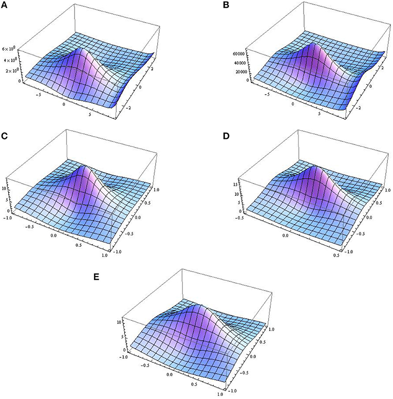
Figure 1. 3D graphical representations of first-order rogue waves. (A) b = 0.5 and δ₀(t) = 0.5, (B) b = 0.79 and δ₀(t) = 0.61, (C) ${\delta }_0(t)=0.5t^2$ and δ(t) = 0.7 + 0.9 cos(0.1t), (D) ${\delta }_0(t)=0.35t^2$ and δ(t) = 0.86 + 1.2 cos(0.1t), and (E) ${\delta }_0(t)=0.35t^2$, δ(t) = 0.1 + 1.2 cos(0.1t), and ${\delta }_0(t)=0.35t^2$.

The results show that there are no different effects of GF on first- and second-order rogue waves. Graphical representations of the amplitude given by Equation (31) at a₀ = 1 and γ(t) = sin³(0.005t) with different values of GF and δ₀(t) is depicted in Figures 2A–C. Six small peaks appear around the one high peak of the second-order solution. Graphical representations of second-order rogue waves with both GF and EMF are also shown in Figures 2D–F.

FIGURE 2

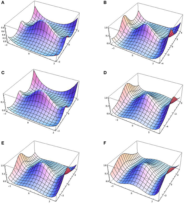
Figure 2. 3D graphical representations of second-order waves. (A) δ(t) = 0.5 and δ₀(t) = 0.1, (B) δ(t) = 0.4 and δ₀(t) = 0.1, (C) δ(t) = 0.7 and δ₀(t) = 0.2 exp(sech(0.2t)), (D) δ(t) = 0.5sech(0.2t) and δ₀(t) = 0.5 exp(sech(0.2t)), (E) δ(t) = 0.5 + 1.2 cos(0.005t) and ${\delta }_0(t)=0.35t^2$, and (F) δ(t) = 0.1 + 1.2 cos(0.1t) and ${\delta }_0(t)=0.35t^2$.

Graphical representations of the amplitudes given by equation (30) at a₀ = 1 and γ(t) = t are depicted in Figures 3A–D with the different parameter values. The curves in Figures 3A,B are formed under the GF, and those in Figures 3C,D are formed when both the GF and EMF are present.

FIGURE 3

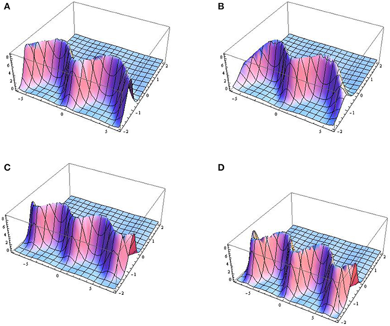
Figure 3. 3D graphical representations of first-order rogue waves. The figures correspond with (A) b = 1.3, δ₀(t) = exp(0.5 + 0.5 cos t) and α = tan²(0.02t), (B) b = 1.5, δ₀(t) = exp(0.05 + 0.5 cos t) and α = tan²(0.02t), (C) δ(t) = 1.4 + 0.05 cos t, δ₀(t) = exp(0.002 + 0.4 cos t) and α = tan²(0.02t), and (D) δ(t) = 1.3 + 0.01 cos t, δ₀(t) = exp(0.05 + 0.5 cos t), and α = tan²(0.02t).

Graphical representations of the amplitude given by Equation (31) at a₀ = 1 and γ(t) = t with different values of GF and δ₀(t) are depicted in Figures 4A,B. Small lumps appear in the graph of the second-order solution. Graphical demonstrations of second-order rogue waves with both GF and EMF are shown in Figures 4C,D.

FIGURE 4

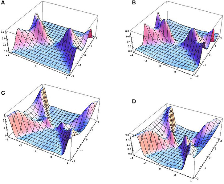
Figure 4. 3D graphical representations of second-order rogue waves. These are constructed with (A) b = 0.9, δ₀(t) = 0.001t and α = 5 tan²(0.05t), (B) b = 0.9, δ₀(t) = 0.001t and α = 5 tan²(0.05t), (C) δ(t) = 1.5 + 0.4 cos t, δ₀(t) = 0.001t and α = 25 tan²(0.05t), and (D) δ(t) = 1.5 + 0.001 cos t, δ₀(t) = 0.001t and α = 35 tan²(0.05t).

6. Conclusion

This article studies the construction of rogue waves in NLSE with a variable coefficient in the presence of harmonic potential. The graphical demonstration shows that the dynamical behavior of waves under the influence of gravity and magnetic fields in linear potential. It is observed that in the presence of GF, the density remains constant, while peak height and width remain invariant. The obtained solutions are of first and second order and are constructed using the ST approach. Moreover, the MI is calculated and is significantly affected by incident optical power.

Author Contributions

All authors listed have made a substantial, direct and intellectual contribution to the work, and approved it for publication.

Conflict of Interest

The authors declare that the research was conducted in the absence of any commercial or financial relationships that could be construed as a potential conflict of interest.

References

1. Akhmediev N, Ankiewicz A, Soto CJM, Rogue waves and rational solutions of the nonlinear Schrödinger equation. Phys Rev E. (2009) 80:026601. doi: 10.1103/PhysRevE.80.026601

PubMed Abstract | CrossRef Full Text | Google Scholar

2. Ali S, Younis M, Ahmad MO, Rizvi STR. Rogue wave solutions in nonlinear optics with coupled Schrdinger equations. Opt Quant Electr. (2018) 50:266. doi: 10.1007/s11082-018-1526-9

CrossRef Full Text | Google Scholar

3. Younas B, Younis M, Ahmed MO, Rizvi STR. Exact optical solitons in (n + 1)- dimensions under anti-cubic law of nonlinearity. Optik. (2018) 156:479–86. doi: 10.1016/j.ijleo.2017.11.148

CrossRef Full Text | Google Scholar

4. Seadawy AR. Nonlinear wave solutions of the three-dimensional Zakharov-Kuznetsov-Burgers equation in dusty plasma. Physica A. (2015) 439:124–31. doi: 10.1016/j.physa.2015.07.025

CrossRef Full Text | Google Scholar

5. Seadawy AR. Three-dimensional nonlinear modified Zakharov-Kuznetsov equation of ion-acoustic waves in a magnetized plasma. Comput Math Appl. (2016) 71:201–12. doi: 10.1016/j.camwa.2015.11.006

CrossRef Full Text | Google Scholar

6. Seadawy AR Two-dimensional interaction of a shear flow with a free surface in a stratified fluid and its solitary-wave solutions via mathematical methods. Eur Phys J Plus. (2017) 132:518. doi: 10.1140/epjp/i2017-11755-6

CrossRef Full Text | Google Scholar

7. Seadawy AR. Three-dimensional weakly nonlinear shallow water waves regime and its traveling wave solutions. Int J Comput Methods. (2018) 15:1850017. doi: 10.1142/S0219876218500172

CrossRef Full Text | Google Scholar

8. Zabusky NJ, Galvin CJ. Shallow-waterwaves, the korteweg-de-vries equation and solitons. J. Fluid Mech. (1971) 47:811–24. doi: 10.1017/S0022112071001393

CrossRef Full Text | Google Scholar

9. Seadawy AR, Rashidy KE, Nonlinear Rayleigh–Taylor instability of the cylindrical fluid flow with mass and heat transfer. Pramana J Phys. (2016) 87:20. doi: 10.1007/s12043-016-1222-x

CrossRef Full Text | Google Scholar

10. Seadawy AR. Stability analysis solutions for nonlinear three-dimensional modified Korteweg-de Vries-Zakharov-Kuznetsov equation in a magnetized electron-positron plasma. Physica A. (2016) 455:44–51. doi: 10.1016/j.physa.2016.02.061

CrossRef Full Text | Google Scholar

11. Seadawy AR. Ion acoustic solitary wave solutions of two-dimensional nonlinear Kadomtsev-Petviashvili-Burgers equation in quantum plasma. Math Methods Appl Sci. (2017) 40:1598–607. doi: 10.1002/mma.4081

CrossRef Full Text | Google Scholar

12. Seadawy AR, Alamri SZ. Mathematical methods via the nonlinear two-dimensional water waves of Olver dynamical equation and its exact solitary wave solutions. Results Phys. (2018) 8:286–91. doi: 10.1016/j.rinp.2017.12.008

CrossRef Full Text | Google Scholar

13. Seadawy AR. Solitary wave solutions of two-dimensional nonlinear Kadomtsev-Petviashvili dynamic equation in dust-acoustic plasmas. Pramana J Phys. (2017) 89:1–11. doi: 10.1007/s12043-017-1446-4

CrossRef Full Text | Google Scholar

14. Seadawy AR. Stability analysis for Zakharov-Kuznetsov equation of weakly nonlinear ion-acoustic waves in a plasma. Comput Math Appl. (2014) 67:172–80. doi: 10.1016/j.camwa.2013.11.001

CrossRef Full Text | Google Scholar

15. Seadawy AR. Stability analysis for two-dimensional ion-acoustic waves in quantum plasmas. Phys Plasmas. (2014) 21:052107. doi: 10.1063/1.4875987

CrossRef Full Text | Google Scholar

16. Ali S, Rizvi STR, Younis M. Traveling wave solutions for nonlinear dispersive water wave systems with time dependent coefficients. Nonliner Dyn. (2015) 82:1755–62. doi: 10.1007/s11071-015-2274-z

CrossRef Full Text | Google Scholar

17. Yue WY, Qing DC. Spatiotemporal Rogue Waves for the Variable-Coefficient (3 + 1)-dimensional nonlinear Schrödinger equation. Commun Theor Phys. (2012) 58:255–60. doi: 10.1088/0253-6102/58/2/15

CrossRef Full Text | Google Scholar

18. Cheemaa N, Younis M. New and more general traveling wave solutions for nonlinear Schrdinger equation. Waves Random Comp Media. (2016) 26:30–41. doi: 10.1080/17455030.2015.1099761

CrossRef Full Text | Google Scholar

19. Wang XB, Tian SF, Qin CY, Zhang TT. Dynamics of the breathers, rogue waves and solitary waves in the (2+1)-dimensional Ito equation. Appl Math Lett. (2017) 68:40–7. doi: 10.1016/j.aml.2016.12.009

CrossRef Full Text | Google Scholar

20. Feng LL, Tian SF, Wang XB, Zhang TT. Rogue waves, homoclinic breather waves and soliton waves for the (2+1)-dimensional B-type Kadomtsev-Petviashvili equation. Appl Math Lett. (2017) 65:90–7.

Google Scholar

21. Younis M, Rizvi STR, Ali S. Analytical and soliton solutions: nonlinear model of nanobioelectronics transmission lines. Appl Math Comput. (2015) 265:994–1002. doi: 10.1016/j.amc.2015.05.121

CrossRef Full Text | Google Scholar

22. Rizvi STR, Ali K, Bashir S, Younis M, Ashraf R, Ahmad MO. Exact soliton of (2+1)-dimensional fractional Schrödinger equation. Superlatt Microstruct. (2017) 107:234–9. doi: 10.1016/j.spmi.2017.04.029

CrossRef Full Text | Google Scholar

23. Xia T, Chen X, Chen D. Darboux transformation and soliton-like solutions of nonlinear Schrödinger equations. Chaos Soltons Fract. (2005) 26:889–96. doi: 10.1016/j.chaos.2005.01.030

CrossRef Full Text | Google Scholar

24. Wang XB, Tian SF, Qin CY, Zhang TT. Characteristics of the breathers, rogue waves and solitary waves in a generalized (2+1)-dimensional Boussinesq equation. Europhys Lett. (2016) 115:10002. doi: 10.1209/0295-5075/115/10002

CrossRef Full Text | Google Scholar

25. Agrawal GP, Baldeck PL, Alfano RR. Modulation instability induced by cross-phase modulation in optical fibers. Phys Rev A. (1989) 39:3406–413. doi: 10.1103/PhysRevA.39.3406

PubMed Abstract | CrossRef Full Text | Google Scholar

26. Tchier F, Yusuf A, Aliyu AI, Inc M. Soliton solutions and conservation laws for lossy nonlinear transmission line equation. Superlatt Microstruct. (2017) 107:320–36. doi: 10.1016/j.spmi.2017.04.003

CrossRef Full Text | Google Scholar

27. Inc M, Yusuf A, Aliyu AI, Baleanu D. Fractional optical solitons for the conformable space-time nonlinear Schro-dinger equation with Kerr law nonlinearity. Opt Quant Elect. (2018) 50:139. doi: 10.1007/s11082-018-1410-7

CrossRef Full Text | Google Scholar

28. Inc M, Yusuf A, Aliyu AI, Hashemi MS. Soliton solutions, stability analysis and conservation laws for the brusselator reaction diffusion model with time- and constant-dependent coefficients. Eur Phys J Plus. (2017) 133:168. doi: 10.1140/epjp/i2018-11989-8

CrossRef Full Text | Google Scholar

29. Yusuf A, Inc M, Bayram M. Invariant and simulation analysis to the time fractional Abrahams- Tsuneto reaction diffusion system. Phys Script. (2019) 94:125005. doi: 10.1088/1402-4896/ab373b

CrossRef Full Text | Google Scholar

30. Yusuf A, Inc M, Baleanu D. Optical solitons with M-truncated and beta derivatives in nonlinear optics. Front Phys. (2019) 7:126. doi: 10.3389/fphy.2019.00126

CrossRef Full Text | Google Scholar

31. Inc M, Aliyu AI, Yusuf A, Baleanu D. Optical solitary waves, conservation laws and modulation instability analysis to the nonlinear Schrödingers equation in compressional dispersive Alven waves. Optik. (2017) 155:257–66. doi: 10.1016/j.ijleo.2017.10.109

CrossRef Full Text | Google Scholar

32. Inc M, Aliyu AI, Yusuf A, Baleanu D. Dispersive optical solitons and modulation instability analysis of Schrödinger-Hirota equation with spatio-temporal dispersion and Kerr law nonlinearity. Superlatt Microstruct. (2018) 113:319–27. doi: 10.1016/j.spmi.2017.11.010

CrossRef Full Text | Google Scholar

33. Yan ZY. Constructive Theory and Applications of Complex Nonlinear Waves. Beijing: Science Press (2007).

Google Scholar

34. Inc M, Aliyu AI, Yusuf A, Baleanu D. Novel optical solitary waves and modulation instability analysis for the coupled nonlinear Schröodinger equation in monomode step-index optical fibers. Superlatt Microstruct. (2018) 113:745–53. doi: 10.1016/j.spmi.2017.12.010

CrossRef Full Text | Google Scholar