Landscape Population Genomics of Forsythia (Forsythia suspensa) Reveal That Ecological Habitats Determine the Adaptive Evolution of Species

Understanding the genetic mechanisms of adaptation to environmental variables is a key concern in molecular ecology and evolutionary biology. Determining the adaptive evolutionary direction and evaluating the adaptation status of species can improve our understanding of these mechanisms. In this study, we sampled 20 populations of Forsythia suspensa to infer the relationship between environmental variables and adaptive genetic variations. Population structure analysis revealed that four genetic groups of F. suspensa exist resulting from divergent selection driven by seven environmental variables. A total of 26 outlier loci were identified by both BayeScan and FDIST2, 23 of which were environment-associated loci (EAL). Environmental association analysis revealed that the environmental variables related to the ecological habitats of F. suspensa are associated with high numbers of EAL. Results of EAL characterization in F. suspensa are consistent with the hypothesis that ecological habitats determine the adaptive evolution of this species. Moreover, a model of species adaptation to environmental variables was proposed in this study. The adaptation model was used to further evaluate the adaptation status of F. suspensa to environmental variables. This study will be useful to help us in understanding the adaptive evolution of species in regions lacking strong selection pressure.

Introduction

Understanding the genetic mechanisms of adaptation to environmental variables is a key issue in molecular ecology and evolutionary biology. Changes in environmental variables are mainly manifested in climate fluctuations on a time scale and in environmental heterogeneity on a spatial scale. Two adaptation strategies are usually adopted by plants in response to environmental variables. One strategy is adjustment in the distribution, and the other is production of adaptive variations in the genome (Davis and Shaw, 2001; Lei et al., 2015). Plants displaying highly efficient seed dispersal capacity often adopt the first strategy as confirmed by phylogeographical studies (Avise, 2009; Hickerson et al., 2010). Conversely, species lacking effective seed dispersal mechanisms are compelled to adapt to local conditions by adopting the second strategy. Substantial adaptive variations in the genome will eventually lead to changes in phenotype and phenological characteristics of a species (Rellstab et al., 2015). These changes provide the basis for adaptive evolution of a species. Interaction between gene flow and natural selection lead to species adaptation in response to heterogeneous regional environment (Rieseberg and Burke, 2001; Ellstrand, 2014), resulting in spatial variation in adaptive allele frequencies among populations (Manel et al., 2012; Schoville et al., 2012). Visualizing adaptive genetic variability across environmental variation is the key in understanding the adaptive evolution of a species (Hoffmann and Willi, 2008). However, detecting adaptive genetic variation remains a great challenge because of the lack of a priori genomic resources for non-model species (Stinchcombe and Hoekstra, 2008).

Joost et al. (2007) have proposed landscape population genomics, which is a relatively new approach used to reveal the relationships between adaptive genetic and environmental variations (Allendorf et al., 2010; Schoville et al., 2012). However, this approach requires genome-wide molecular markers and high-resolution environmental data (Balkenhol et al., 2009; Epperson et al., 2010). To date, amplified fragment length polymorphisms (AFLPs), inter-simple sequence repeats (ISSRs), and genotyping by sequencing are widely used in landscape population genomics studies (De Kort et al., 2014; Rellstab et al., 2015; Wang et al., 2016). High-resolution environmental data are now available from public climate databases, such as the WORLDCLIM database (www.worldclim.org). Recent landscape population genomics studies have highlighted the genetic mechanisms of species adaptation to the environment (Ćalić et al., 2016; Pluess et al., 2016). Statistical approaches have been developed to identify outlier loci showing higher differentiation among populations and lower genetic diversity within populations compared with selectively neutral regions of a genome (Abebe et al., 2015); these approaches include BayeScan based on multinomial-Dirichlet model (Foll and Gaggiotti, 2008) and Arlequin based on hierarchical island model (Excoffier and Lischer, 2010). To further determine whether these outlier loci are driven by environmental factors, researchers have developed multiple statistical approaches for association testing; these approaches include Bayesian linear mixed model (Coop et al., 2010; Günther and Coop, 2013), generalized dissimilarity model (Ferrier et al., 2007), generalized estimating equation (Carl and Kuhn, 2007), latent factor mixed model (Frichot et al., 2013), multiple logistic regression analyses (Grivet et al., 2011), and spatial analyses based on univariate logistic regression (Joost et al., 2007).

Although a large number of adaptive loci driven by environmental variables were identified in more than one species, the general and overall result taken from these landscape population genomics studies in regional vegetation is that the commonality on species adaptation response to identical environmental variables is still unclear. Commonality in adaptive evolution in regional vegetation generally requires extremely strong selection pressure produced by one or more environmental variables. Species exposed to extreme heat and drought in desert areas or to high salinity in the ocean tend to produce convergent adaptive evolution in genes or phenotype (Kültz, 2015; Givnish, 2016). However, most regions do not exhibit strong selection pressure produced by these extreme environments mentioned above. Thus, the direction of adaptive evolution in regional vegetation is usually diverse (Manel et al., 2012; Ćalić et al., 2016). Determining the direction of adaptive evolution of the genome driven by environmental variables is an interesting endeavor. Another interesting concern is the means by which the adaptation status of species in response to environmental variables can be evaluated. Understanding the commonality of this diverse adaptive evolution of regional vegetation is useful in developing suitable conservation and management strategies.

The warm temperate zone in China is located between 32°30′–42°30′ and 103°30′–124°10′ (Shangguan et al., 2009). The typical vegetation in this region consists of deciduous broad-leaved forest (Gao et al., 2001). This region does not exert strong selection pressure brought about by extreme environmental variables. In this study, we sampled Forsythia suspensa (Thunb.) Vahl (Oleaceae), a deciduous shrub widespread at 300–2,200 m above sea level in the warm temperate zone in China. The flowering period of F. suspensa is from March to June, and the fruiting period is from July to September. This species prefers light and tolerates a certain degree of shade; additionally, it prefers warm and humid climate and can tolerate cold and drought but not waterlogging (Niu et al., 2003). We sampled 20 natural populations of F. suspensa in the warm temperate zone in China to infer the relationship between environmental variables and adaptive genetic variations. Start codon targeted (SCoT) polymorphism is a gene-targeted marker, which was developed based on short conserved start codon in plant genes (Collard and Mackill, 2009). SCoT markers are highly variable and reproducible and have been widely used to survey population genetics and phylogenetics (Guo et al., 2014; Feng et al., 2015; Sorkheh et al., 2016). However, SCoT markers have been seldom used in landscape population genomics to detect adaptive loci in genomes.

In this study, we used environmental data and 1,242 loci yielded by SCoT markers to study the adaptive evolution of F. suspensa in the warm temperate zone in China. The present study aimed to (i) reveal the spatial genetic structure of F. suspensa, (ii) identify the key environmental variables that drive adaptive differentiation in F. suspensa, and (iii) evaluate the adaptation status of the species in response to environmental variables.

Methods

Sample Collection

A total of 204 individuals from 20 natural populations were collected from the entire distribution range of F. suspensa in China (Figure 1). Most population samples contained 10–12 individuals (Table 1). Although 10–12 individuals of one population might not be an ideal sample size, the sample numbers could meet the needs of genetic analysis to overcome sampling bias (De Kort et al., 2014). All individuals were collected when the population size was <10. Thus, those populations with fewer individuals sufficiently represented their genetic diversity. Fresh leaves were collected and stored in silica gel at room temperature until DNA extraction. Table 1 shows the geographical coordinates of the sampled populations.

FIGURE 1

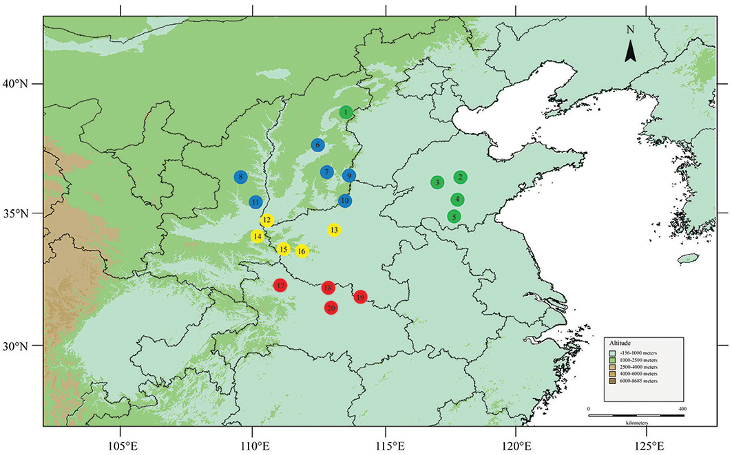
Figure 1. Locations of the 20 sampled F. suspensa populations. Map produced by software DIVA-GIS 7.5.0, URL: http://www.diva-gis.org/download/.

TABLE 1

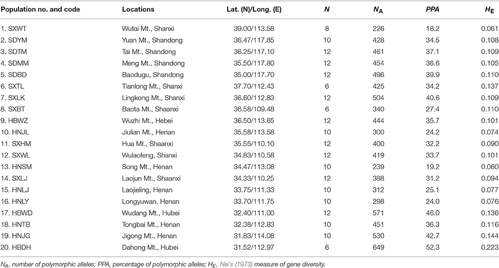
Table 1. Details of population locations, sample size, genetic diversity of 20 populations for F. suspensa.

Molecular Protocols

Genomic DNA was extracted from ~30 mg of dried leaves by using a Plant DNA Extraction Kit DP305 (Tiangen, Beijing, China) according to the manufacturer's recommendations. DNA concentration and quality were measured using a Microcolume Spectrophotometer ND5000 (BioTeke, Beijing, China). After preliminary screening of 36 SCoT primers (Collard and Mackill, 2009), 10 primers (SCoT4, SCoT5, SCoT6, SCoT9, SCoT12, SCoT14, SCoT17, SCoT18, SCoT21, and SCoT31) were selected for polymerase chain reaction (PCR). SCoT4, SCoT5, and SCoT21 were 5′ fluorescent primers labeled with FAM; SCoT9, SCoT17, and SCoT18 were labeled with HEX; SCoT6, SCoT12, SCoT14, and SCoT31 were labeled with TAMRA. PCR amplification was performed in a 20 μL reaction mixture consisting of 20 ng of template DNA, 10 mM reaction buffer (pH 8.3), 0.2 mM dNTPs, 0.3 μM primer, and 1 unit of Taq polymerase (Tiangen, Beijing, China). PCRs were performed in an iCycler gene amplification system (Bioteke, Beijing, China) under the following conditions: initial denaturation for 4 min at 95°C followed by 35 cycles of denaturation for 40 s at 94°C, primer annealing for 45 s at a primer-specific annealing temperature (48°C for SCoT21, 52°C for SCoT4, SCoT5, SCoT6, SCoT9, SCoT12, and SCoT17, 55°C for SCoT31, and 60°C for SCoT14 and SCoT18), extension for 1 min at 72°C with a subsequent extension step for 5 min at 72°C, and termination by a final hold at 4°C. PCR products were mixed with 10 μL of HiDi formamide and separated on an ABI 3730 DNA Analyzer at BGI (Beijing, China). PCR products were sized relative to ROX1000 size standard (Applied Biosystems, Foster City, USA).

Data Analysis

Unambiguous SCoT fragments were scored and transformed into a 1/0 matrix according to the presence or absence of peaks viewed using GeneMarker 2.2.0 (SoftGenetics, State College, Pennsylvania, USA). To reduce the scoring false rate, we scored the peaks within 60–1,000 bp and heights above 500 relative fluorescent units. Subsequent population genetic analyses were performed on the basis of this 1/0 character matrix.

Genetic parameters per population were calculated by AFLPSURV 1.0 (Vekemans, 2002). The estimates included the number of polymorphic alleles (N_A), percentage of polymorphic alleles (PPA), gene diversity of Nei (H_E; Nei, 1973), pairwise Nei's unbiased genetic distance (Nei, 1987; Lynch and Milligan, 1994) between populations, and gene frequencies per allele in each population.

Genetic structure of the 20 populations of F. suspensa was assessed using the procedures NEIGHBOR and CONSENSE within the program PHYLIP 3.63 (Felsenstein, 2004). Population differentiation was characterized using hierarchical and non-hierarchical analysis of molecular variance (AMOVA) within ARLEQUIN 3.5.1.2 (Excoffier and Lischer, 2010). To infer the contribution of geographical distance to spatial genetic structure, we performed mantel tests of isolation-by-distance (IBD) in IBD 3.23 (Jensen et al., 2005) by regressing the Nei's unbiased genetic distance against geographical distance. In this study, the strong correlated environmental variables (r > 0.95) were excluded and the uncorrelated environmental variables were used for further analyses. Auto correlation analysis of environmental variables was performed using Pearson's regression in SPSS 19 (SPSS Inc., Chicago, IL, USA). Ten environmental variables (Bio2, Bio3, Bio4, Bio5, Bio6, Bio8, Bio12, Bio13, Bio15, and Bio17) were identified as uncorrelated environmental variables. To further infer the contribution of environmental variables to spatial genetic structure, we performed redundancy analysis (RDA) by using CANOCO 4.5 (Ter Braak and Smilauer, 2002). In RDA, gene frequencies per allele in each population (Table S1) were used as response variable, and the 10 uncorrelated environmental variables (Tables S2, S3) were used as explanatory variables. Environmental data from 1950 to 2000 at 2.5 arcmin resolution were obtained from the world climate database (http://www.diva-gis.org/climate). Environmental data for each population were extracted using DIVA-GIS 7.5 (Hijmans et al., 2001).

To identify outlier loci, we utilized a Bayesian approach based on the method described by Beaumont and Balding (2004) by using BayeScan 2.1 (Foll and Gaggiotti, 2008). The outliers were calculated using the following parameters: a sample size of 5,000, thinning interval of 10, 20 pilot runs with a run length of 5,000, and additional burn-in of 50,000 iterations. Posterior probability >0.76 corresponding to log₁₀-values of the posterior odds (PO) >0.5 were taken as substantial evidence for selection. Thus, the above mentioned loci were regarded as outlier loci. The second approach was based FDIST2 approach proposed by Beaumont and Nichols (1996) by using Arlequin 3.5.1.2 (Excoffier and Lischer, 2010). The outliers were calculated with a hierarchical island model using the following parameters: 100 simulated demes and 20,000 coalescent simulations. To reduce the false discovery rate, loci with minor allele frequency <5% were excluded. The loci outside the 95% confidence interval were regarded as outlier loci. To further test whether these outlier loci are driven by environmental variables, we conducted an environmental association analysis based on latent factor mixed model (LFMM) by using LFMM 1.2 (Frichot et al., 2013). Given that the Bayesian mixed model considers the population structure, this model can avoid the bias caused by population history and isolation by distance and yields a robust result for environment-associated loci (EAL). The association analysis was run using the following parameters: 10,000 sweeps, 1,000 burn-in sweeps, and the number of latent factors used was recommended by PHYLIP. The loci with |z| > 3 and P < 0.001 were regarded as EAL.

Results

Genetic Structure

Ten SCoT primers were selected to investigate the population genetic structure of F. suspensa. A total of 1,242 unambiguous loci were identified with sizes ranging from 60 to 1,000 bp. The number of loci in 10 primers ranged from 60 (SCoT31) to 161 (SCoT4). The gene diversity of Nei (H_E) at the species level was 0.124. The lowest number of polymorphic alleles (N_A = 226, PPA = 18.2) was exhibited in SXWT (P1) population and the highest (N_A = 649, PPA = 52.3) in HBDH (P20) population. The lowest gene diversity of Nei (H_E = 0.060) was exhibited in HNSM population and the highest (H_E = 0.223) in HBDH (P20) population. Overall, Table 1 shows the summary statistics of the genetic diversity analyses of 20 populations of F. suspensa.

Populations of F. suspensa were significantly structured as revealed by the clearly population-based NJ network, the 20 populations were subdivided into four genetic groups (Figure 2). The four genetic groups identified were as follows: East group (P1–P5), North group (P6–P11), Middle group (P12–P16), and South group (P17–P20). Non-hierarchical AMOVA (Table 2) revealed significant differences among these populations (F_ST = 0.115, P < 0.001). Despite the clear genetic subdivision in the 20 populations of F. suspensa, only minimal genetic variations existed among these four groups (5.30%, F_CT = 0.053, P < 0.05), and most genetic variations occurred within a population (86.06%, F_ST = 0.139, P < 0.001). Non-significant patterns of isolation-by-distance were detected among the 20 populations of F. suspensa (r = 0.1209, P > 0.05), indicating that geographic distance exerted no significant effect on genetic differentiation. RDA analysis was performed to detect the contribution of environmental variables on spatial genetic structure. The RDA results are shown in Table 3 and Figure 3. Correlations between genetic variables and environmental variables in axes 1 and 2 were 0.953 and 0.976, respectively. The percent variance of the genetic variable-environmental variable relationship in axes 1 and 2 were 26.9 and 19.0%, respectively. RDA results showed that seven environmental variables were significantly associated with RDA axes 1 and 2 (Table 3). Among these seven environmental variables, mean diurnal range (Bio2), temperature seasonality (Bio4), and min temperature of coldest month (Bio6) were related to temperature. Meanwhile, annual precipitation (Bio12), precipitation of the wettest month (Bio13), precipitation seasonality (Bio15), and precipitation of driest quarter (Bio17) were all related to precipitation. Bio12, Bio13, and Bio17 showed the highest correlation among the seven environmental variables.

FIGURE 2

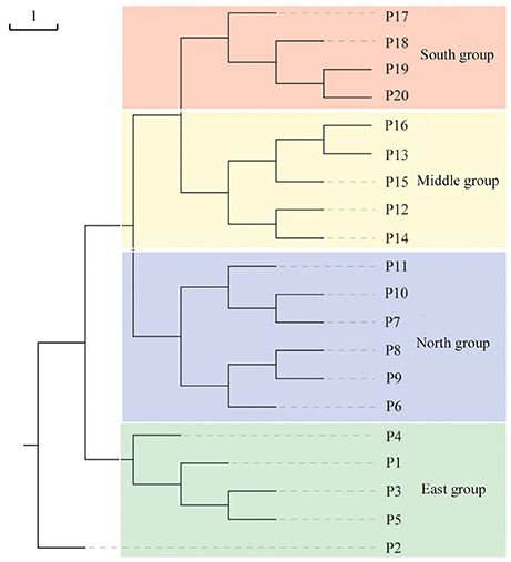
Figure 2. Neighbor-joining network illustrating the genetic relationships among 20 populations of F. suspensa based on Nei's (1987) unbiased genetic distance.

TABLE 2

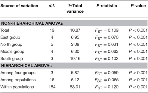
Table 2. Hierarchical AMOVAs for SCoT variation surveyed in F. suspensa.

TABLE 3

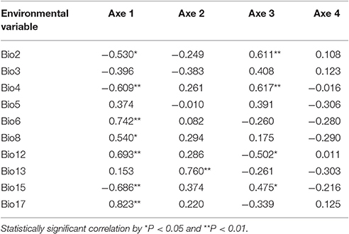
Table 3. Correlations between environmental variables and the ordination axes.

FIGURE 3

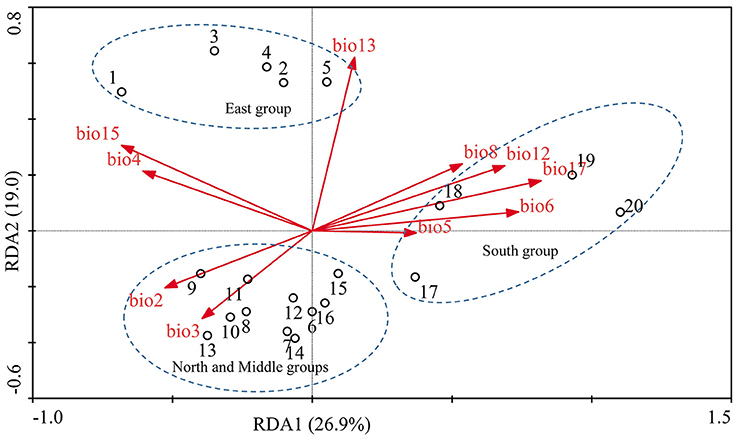
Figure 3. RDA analysis was performed to determine the relative contribution of environmental variations shaping the genetic structure. The biplot depicts the eigenvalues and lengths of eigenvectors for the RDA. Population locations on the spatial axes are marked by their number.

EAL Detection

Using the BayeScan method, 63 outlier loci were identified (5.1% of the total number of SCoT loci) with a posterior probability of higher than 0.76 (i.e., log₁₀ PO > 0.5), which is a threshold for substantial evidence under selection (Table S4). Using the FDIST2 method, a relatively relaxed result of 132 outlier loci (10.6% of the total number of SCoT loci) above the 95% threshold were identified (Table S4). Based on the results yielded by two identified methods, a total of 26 common loci were detected by both methods, which represented more true outlier loci (Figure 4). To further reduce the false discovery rate, we used the 26 common loci for environmental association analyses. Among these outlier loci, 23 environment-associated loci (EAL; 1.9% of the total number of SCoT loci) associated with at least one environmental variable was detected in F. suspensa by using LFMM (Table 4). Among these detected EAL, 20 were significantly associated with both temperature and precipitation, three were significantly associated with precipitation (Table 4). Among the 10 environmental variables, Bio13, Bio15, and Bio6 were associated with the highest numbers of EAL, which indicated that these environmental variables might play more important roles in adaptive evolution in F. suspensa (Table 4).

FIGURE 4

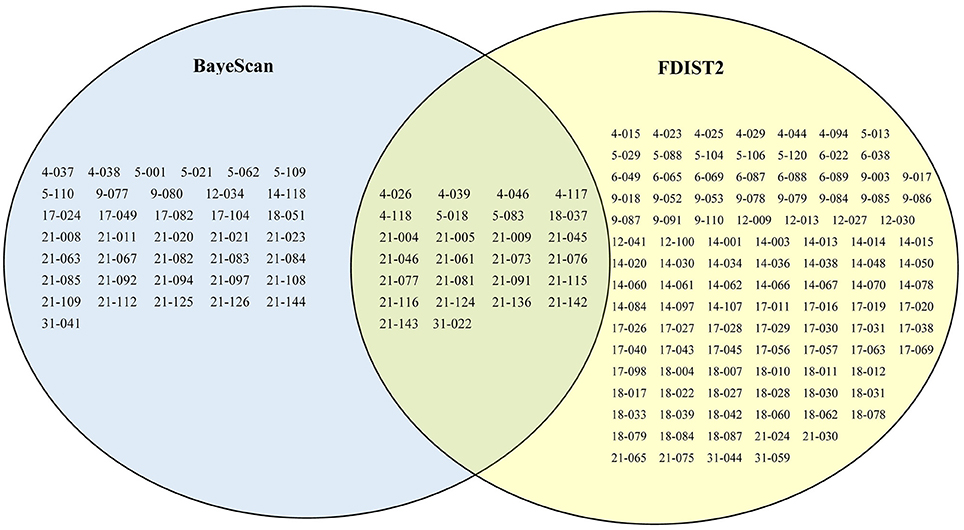
Figure 4. The results of outlier loci identified by Bayescan and Arlequin. Sixty-three, one hundred and thirty-two, and twenty six loci were detected as outlier loci in F. suspensa using Bayescan, Arlequin, and both with Bayescan and Arlequin, respectively.

TABLE 4

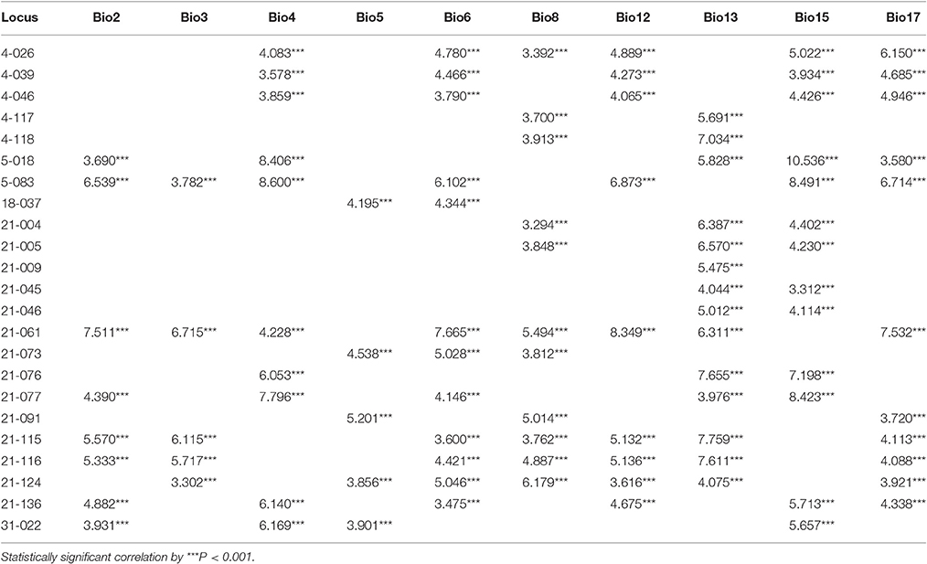
Table 4. The EAL as indicated by |z|-score.

Discussion

By using 1,242 SCoT loci, we analyzed the adaptive evolution of F. suspensa in response to environmental variables. SCoT markers present the advantages of high throughput, non-neutral bias, and non-requirement for a priori genomic information (Deng et al., 2015). Thus, SCoT markers are very suitable for adaptive loci detection. However, markers are seldom applied in landscape population genomics. To date, the genome information of F. suspensa (2n = 26) is still unknown. According to a high-density genetic linkage map in the related species of Olea europaea (2n = 46), 5,643 markers produced a high resolution map of 0.53 cM (İpek et al., 2016). Although a smaller number of markers were used in this study, the overall outlier detection rate in F. suspensa was 5.1% in BayeScan and 10.6% in FDIST2. These rates are considered with those reported in other studies, such as 2.85% in Alnus glutinosa (De Kort et al., 2014) and 4.5% in Picea mariana (Prunier et al., 2011) as determined using SNPs, 4.22% in Cephalotaxus oliveri (Wang et al., 2016) as determined using ISSRs, and 9% in Arabis alpina (Poncet et al., 2010) and 10% in 13 alpine species (Manel et al., 2012) as determined using AFLPs. Although SCoT markers are non-neutral biased, their detection rates in this study are not significantly higher than that of other molecular markers.

Understanding the spatial population genetic structure of species is a key concern in landscape population genomics (Schoville et al., 2012; Hall and Beissinger, 2014). In recent years, research on the influence of environmental variables on spatial structure gradually increased. Identifying the influence of environmental variables on spatial genetic structure remains difficult because of the complex reciprocal interactions of multiple factors (Chung et al., 2004; Ohsawa and Ide, 2008). Our survey demonstrated a significant spatial population genetic structure across the studied populations. These populations could be divided into four genetic groups, namely, East group (P1–P5), North group (P6–P11), Middle group (P12–P16), and South group (P17–P20). Three possible hypotheses can explain the genetic divergence of these populations. First, the current spatial genetic structure resulted from the mixing of the four gene pools. Second, geographical barriers occurred among the four genetic groups, and these barriers blocked the gene flow and ultimately led to genetic differentiation of the four groups. Third, the four groups were exposed to significantly varying environmental conditions, and divergent selection caused by these heterogeneous environmental variables led to genetic divergence of the four groups. Assuming that the first hypothesis is reasonable, high genetic diversity can be expected in populations located at the contact zone. However, results of the genetic diversity index based on SCoT data did not support this explanation. Similarly, the populations (P1, P9, P11, P12, P16, and P17) located at the contact zone of the four groups did not show the expected high genetic diversity. Moreover, F. suspensa displays strong pollen dispersal ability, resulting in a high pollen-mediated gene flow among the populations (Fu et al., 2014). The non-significant patterns of IBD in F. suspensa also confirmed the strong gene flow among the populations. Long-term strong gene flow among populations would result in a consistent population genetic background. However, the results for population structure are inconsistent with the expected strong gene flow. Thus, the first hypothesis failed to explain the genetic divergence of F. suspensa. Assuming that the genetic divergence in F. suspensa can be explained by the second hypothesis, we expect to observe considerable genetic divergence among the four groups, with sufficiently strong geographic barrier separating these groups from one another. However, the result of non-hierarchical AMOVA did not support this hypothesis, and only 5.87% genetic variation was observed among the four groups. More importantly, we did not find significant geographical barriers, i.e., mountains and rivers, which separate the four groups. Therefore, the second hypothesis apparently cannot explain the genetic divergence in F. suspensa. Assuming that the third hypothesis applies in F. suspensa, a shallow genetic divergence among the four groups would be expected because of the interaction between strong gene flow and significant natural selection by environmental variables. The result of non-hierarchical AMOVA (F_CT = 0.059) was consistent with this expectation. We then performed RDA to test whether the genetic subdivision of the four groups was caused by environmental factors. The RDA results indicated that seven environmental variables related to temperature and precipitation significantly contributed to the spatial genetic structure of F. suspensa. Among these environmental variables, Bio12, Bio13, and Bio17 were the most important environmental factors that have shaped the spatial genetic structure of F. suspensa. Moreover, RDA results showed that these environmental variables could clearly divide the populations into East group, South group, and the combined Middle and North groups (Figure 3). These findings showed that environmental variables greatly influenced the spatial genetic structure of F. suspensa. However, other unknown factors have possibly led to the eventual divergence of the Middle and North groups. Overall, our results for F. supsensa support the third hypothesis.

Landscape genomics studies have devoted more attention to the identification of adaptive gene loci (Rellstab et al., 2015; Shryock et al., 2015). However, less attention has been devoted to the environmental variables affecting the adaptive evolution of species. Under extreme environments, a strong selection pressure will facilitate convergent evolution of species (Azua-Bustos et al., 2012). The environmental variables driving the convergent evolution of species in these regions are usually common (Kültz, 2015; Givnish, 2016). However, extreme environmental variables are inexistent in most vegetation distribution areas. In regions lacking extreme environmental variables, the direction of adaptive evolution of the genome is uncertain, and the environmental variables driving their adaptive evolution vary. Thus, identifying whether commonality exists among these environmental variables in driving diverse adaptive evolution of species is important.

In this study, we chose F. suspensa as a model to address the above mentioned concerns. This species is distributed in the warm temperate zone in China, and this zone lacks strong selection pressure. We hypothesized that ecological habitats determine adaptive evolution of species and drive the genome to generate a large number of EAL. Thus, understanding the ecological habitats of F. suspensa is urgent. In this study, we focused on the ecological habitats related to temperature and precipitation. F. suspensa prefers warm and humid climate and can tolerate cold and drought but not waterlogging (Niu et al., 2003). Among the adopted environmental variables, Bio12 was associated with the ecological habitat of “prefer humidity”; Bio6 was associated with the ecological habitat of “tolerate cold”; Bio17 was associated with the ecological habitat of “tolerate drought”; and Bio13 was associated with the ecological habitat of “avoid waterlogging.” Most of the time, the warmest and wettest seasons in the warm temperate zone in China overlap, and the same is true for the coldest and driest seasons. The results of LFMM expectedly showed that the ecological habitat of “avoid waterlogging” (Bio13) were associated with the highest number of EAL; the ecological habitat of “tolerate cold” (Bio6), and “tolerate drought” (Bio17) were associated with increased number of EAL. Unexpectedly, Bio4 and Bio15 were also associated with increased number of EAL. This result implies that seasonal variation in temperature and precipitation exerted strong selection pressure on F. suspensa and drove the genome to generate adaptive evolution. However, the ecological habitats of “prefer warmth” and “prefer humidity” was only related to a small number of EAL. Overall, most aspects of the characterized EAL of F. suspensa are consistent with the hypothesis that ecological habitats determine adaptive evolution of a species.

Whether this hypothesis demonstrates a certain degree of universality must be determined. The adaptive evolution of Achyranthes bidentata and Cotinus coggygria in warm temperate zone in China is also associated with their ecological habitats (unpublished data). For A. bidentata, the highest number of EAL is associated with its ecological habitats of “cold intolerance” and “avoiding waterlogging.” For C. coggygria, the highest number of EAL is associated with its ecological habitat of “avoiding waterlogging.” To further confirm the universality of our hypothesis, we reviewed the recent landscape population genomics studies in other regions. For example, the high number of EAL in Picea mariana is related to its ecological habitat of “cold resistance” (Prunier et al., 2011); additionally, EAL is related to “drought resistance” in Alnus glutinosa (De Kort et al., 2014), to “temperature and precipitation sensitivity” in Cephalotaxus oliveri (Wang et al., 2016), and to “drought and cold tolerance” in Abies alba (Roschanski et al., 2016). Based on the above-mentioned evidence, the hypothesis that the ecological habitats determine adaptive evolution of species possibly demonstrate a certain degree of universality.

Despite the lack of extreme environmental variables in the warm temperate zone in China, various environmental factors more or less produce selection pressure on F. suspensa. Therefore, the level of adaptabilities to various environmental variables varies. Another important concern is the evaluation of the adaptation status of species in response to environmental variables. Thus, we propose a model of adaptive evolution of species in response to environmental variables. The adaptive evolution of species was divided into five stages (Figure 5). In stage 1 (S1), environmental variables did not exert selection pressure on the species, and the species did not yield adaptive differentiation. Consequently, EAL could not be detected in the genome. In S2, the altered environmental variables generated selection pressure on the species, and the species genome produced EAL to cope with such selection pressure. Eventually, EAL increased gradually. However, the increased EAL loci were not sufficient to respond to this selection pressure, and species showed sensitivity to this environmental variable at this stage. In S3, the species genome generated an adequate amount of EAL in response to selection pressure. At this stage, species showed adaptability, and this adaptability would be further strengthened with time delay. In S4, selection pressure yielded by environmental variable disappeared or did not occur frequently, and the EAL on the species genome decreased gradually. At this stage, the species was resistant to this environmental variable. In S5, the EAL on the species genome completely disappeared because the selection pressure yielded by this environmental variable has long been inexistent. We used this model to help us identify the adaptation status for F. suspensa in response to various environmental variables. Despite a high number of EAL driven by waterlogging (Bio13), F. suspensa still showed the ecological habitats of “avoid waterlogging.” Thus, the adaptability for F. suspensa in response to waterlogging must have occurred in S2. In the same manner, we detected a high number of EAL associated with cold (Bio6) and drought (Bio17). However, the selection pressure from cold and drought gradually declined and reached a level far below the critical value that F. suspensa can tolerate. For example, the minimum temperature during the coldest month (Bio6) from 1950 to 2000 was −2°C, which was far lower than the minimum temperature that F. suspensa can tolerate (−30°C; Xu et al., 1996). Thus, we speculate that adaptability of F. suspensa to cold and drought occurred in S4. Interestingly, seasonal variation in temperature and precipitation is required as reported by studies on F. suspensa cultivation, whereas numerous EALs are associated with temperature seasonality (Bio4) and precipitation seasonality (Bio15). This phenomenon is possibly consistent with the ecological habitats of F. suspensa, i.e., “prefer humidity” and “tolerate drought,” as well as “prefer warmth” and “tolerate cold.” Overall, the combination of identification of EAL and ecological habitats and our adaptation model is useful in understanding the adaptation of species to various environmental variables.

FIGURE 5

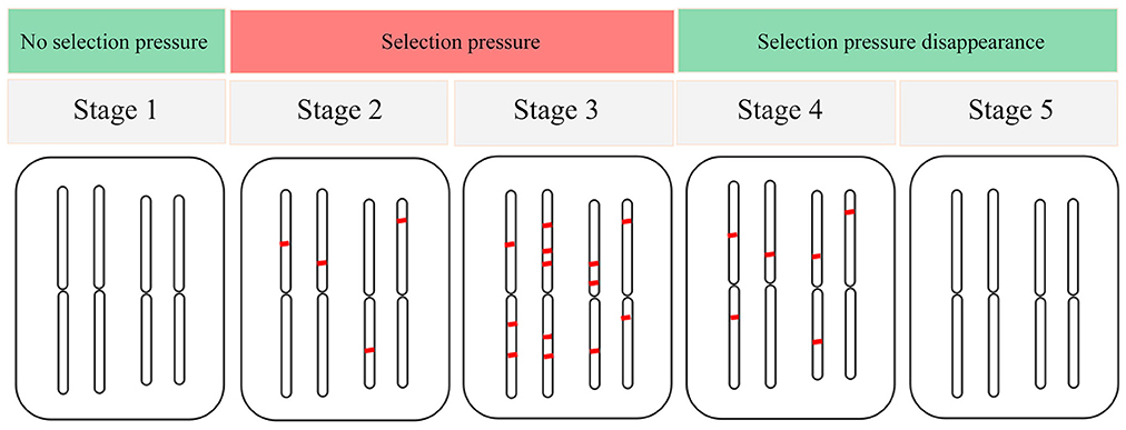
Figure 5. The adaptation model of species in response to environmental variables.

Author Contributions

YL conceived and designed the experiments and wrote the paper; JY and CM performed the experiments and analyzed the data; RM checked English grammar and revised the paper. All authors read and approved the final version of the manuscript.

Conflict of Interest Statement

The authors declare that the research was conducted in the absence of any commercial or financial relationships that could be construed as a potential conflict of interest.

Acknowledgments

This work was supported by the Henan Agricultural University Science and Technology Innovation Fund (KJCX2016A2), the Funding Scheme of Young Backbone Teachers of Higher Education Institutions in Henan Province (2015GGJS-081), and the Key Scientific Research Projects of Henan Higher School (16A220002).

Supplementary Material

The Supplementary Material for this article can be found online at: http://journal.frontiersin.org/article/10.3389/fpls.2017.00481/full#supplementary-material

References

Abebe, T. D., Naz, A. A., and Léon, J. (2015). Landscape genomics reveal signatures of local adaptation in barley (Hordeum vulgare L.). Front. Plant Sci. 6:813. doi: 10.3389/fpls.2015.00813

PubMed Abstract | CrossRef Full Text | Google Scholar

Allendorf, F. W., Hohenlohe, P. A., and Luikart, G. (2010). Genomics and the future of conservation genetics. Nat. Rev. Genet. 11, 697–709. doi: 10.1038/nrg2844

PubMed Abstract | CrossRef Full Text | Google Scholar

Avise, J. C. (2009). Phylogeography: retrospect and prospect. J. Biogeogr. 36, 3–15. doi: 10.1111/j.1365-2699.2008.02032.x

CrossRef Full Text | Google Scholar

Azua-Bustos, A., González-Silva, C., Arenas-Fajardo, C., and Vicuña, R. (2012). Extreme environments as potential drivers of convergent evolution by exaptation: the Atacama Desert Coastal Range case. Front. Microbiol. 3:426. doi: 10.3389/fmicb.2012.00426

PubMed Abstract | CrossRef Full Text | Google Scholar

Balkenhol, N., Waits, L. P., and Dezzani, R. J. (2009). Statistical approaches in landscape genetics: an evaluation of methods for linking landscape and genetic data. Ecography 32, 818–830. doi: 10.1111/j.1600-0587.2009.05807.x

CrossRef Full Text | Google Scholar

Beaumont, M. A., and Balding, D. J. (2004). Identifying adaptive genetic divergence among populations from genome scans. Mol. Ecol. 13, 969–980. doi: 10.1111/j.1365-294X.2004.02125.x

PubMed Abstract | CrossRef Full Text | Google Scholar

Beaumont, M. A., and Nichols, R. A. (1996). Evaluating loci for use in the genetic analysis of population structure. Proc. R. Soc. Lond. B Biol. Sci. 263, 1619–1626. doi: 10.1098/rspb.1996.0237

CrossRef Full Text | Google Scholar

Ćalić, I., Bussotti, F., Martínez-García, P. J., and Neale, D. B. (2016). Recent landscape genomics studies in forest trees—what can we believe? Tree Genet. Genomes 12:3. doi: 10.1007/s11295-015-0960-0

CrossRef Full Text | Google Scholar

Carl, G., and Kuhn, I. (2007). Analyzing spatial autocorrelation in species distributions using Gaussian and logit models. Ecol. Model. 207, 159–170. doi: 10.1016/j.ecolmodel.2007.04.024

CrossRef Full Text | Google Scholar

Chung, M. M., Gelembiuk, G., and Givnish, T. J. (2004). Population genetic variation and phylogeography of endangered Oxytropis campestris var. chartacea and relatives: arctic-alpine disjuncts in eastern North America. Mol. Ecol. 13, 3657–3673. doi: 10.1111/j.1365-294X.2004.02360.x

PubMed Abstract | CrossRef Full Text | Google Scholar

Collard, B. C. Y., and Mackill, D. J. (2009). Start Codon Targeted (SCoT) polymorphism: a simple, novel DNA marker technique for generating gene-targeted markers in plants. Plant Mol. Biol. Rep. 27, 86–93. doi: 10.1007/s11105-008-0060-5

CrossRef Full Text | Google Scholar

Coop, G., Witonsky, D., Di Rienzo, A., and Pritchard, J. K. (2010). Using environmental correlations to identify loci underlying local adaptation. Genetics 185, 1411–1423. doi: 10.1534/genetics.110.114819

PubMed Abstract | CrossRef Full Text | Google Scholar

Davis, M. B., and Shaw, R. G. (2001). Range shifts and adaptive responses to quaternary climate change. Science 292, 673–679. doi: 10.1126/science.292.5517.673

PubMed Abstract | CrossRef Full Text | Google Scholar

De Kort, H., Vandepitte, K., Bruun, H. H., Closset-Kopp, D., Honnay, O., and Mergeay, J. (2014). Landscape genomics and a common garden trial reveal adaptive differentiation to temperature across Europe in the tree species Alnus glutinosa. Mol. Ecol. 23, 4709–4721. doi: 10.1111/mec.12813

PubMed Abstract | CrossRef Full Text | Google Scholar

Deng, L., Liang, Q., He, X., Luo, C., Chen, H., and Qin, Z. (2015). Investigation and analysis of genetic diversity of diospyros germplasms using SCoT molecular markers in Guangxi. PLoS ONE 10:e0136510. doi: 10.1371/journal.pone.0136510

PubMed Abstract | CrossRef Full Text | Google Scholar

Ellstrand, N. C. (2014). Is gene flow the most important evolutionary force in plants? Am. J. Bot. 101, 737–753. doi: 10.3732/ajb.1400024

PubMed Abstract | CrossRef Full Text | Google Scholar

Epperson, B. K., McRae, B. H., Scribner, K., Cushman, S. A., Rosenberg, M. S., Fortin, M. J., et al. (2010). Utility of computer simulations in landscape genetics. Mol. Ecol. 19, 3549–3564. doi: 10.1111/j.1365-294X.2010.04678.x

PubMed Abstract | CrossRef Full Text | Google Scholar

Excoffier, L., and Lischer, H. E. (2010). Arlequin suite ver 3.5: a new series of programs to perform population genetics analyses under Linux and Windows. Mol. Ecol. Resour. 10, 564–567. doi: 10.1111/j.1755-0998.2010.02847.x

PubMed Abstract | CrossRef Full Text | Google Scholar

Felsenstein, J. (2004). PHYLIP Version 3.63. Seattle: Department of Genome Sciences, University of Washington.

Feng, S., He, R., Yang, S., Chen, Z., Jiang, M., Lu, J., et al. (2015). Start codon targeted (SCoT) and target region amplification polymorphism (TRAP) for evaluating the genetic relationship of Dendrobium species. Gene 567, 182–188. doi: 10.1016/j.gene.2015.04.076

PubMed Abstract | CrossRef Full Text | Google Scholar

Ferrier, S., Manion, G., Elith, J., and Richardson, K. (2007). Using generalized dissimilarity modelling to analyze and predict patterns of beta diversity in regional biodiversity assessment. Divers. Distrib. 13, 252–264. doi: 10.1111/j.1472-4642.2007.00341.x

CrossRef Full Text | Google Scholar

Foll, M., and Gaggiotti, O. (2008). A genome scan method to identify selected loci appropriate for both dominant and codominant markers: a Bayesian perspective. Genetics 180, 977–993. doi: 10.1534/genetics.108.092221

PubMed Abstract | CrossRef Full Text | Google Scholar

Frichot, E., Schoville, S. D., Bouchard, G., and Francois, O. (2013). Testing for associations between loci and environmental gradients using latent factor mixed models. Mol. Biol. Evol. 30, 1687–1699. doi: 10.1093/molbev/mst063

PubMed Abstract | CrossRef Full Text | Google Scholar

Fu, Z. Z., Li, Y. H., Zhang, K. M., and Li, Y. (2014). Molecular data and ecological niche modeling reveal population dynamics of widespread shrub Forsythia suspensa (Oleaceae) in China's warm-temperate zone in response to climate change during the Pleistocene. BMC Evol. Biol. 14:114. doi: 10.1186/1471-2148-14-114

PubMed Abstract | CrossRef Full Text | Google Scholar

Gao, X. M., Ma, K. P., and Chen, L. Z. (2001). Species diversity of some deciduous broad-leaved forests in the warm-temperate zone and its relations to community stability. Acta Phytoecol. Sin. 25, 553–559.

Givnish, T. J. (2016). Convergent evolution, adaptive radiation, and species diversification in plants. Encyclopedia Evol. Biol. 362–373. doi: 10.1016/B978-0-12-800049-6.00266-3

CrossRef Full Text

Grivet, D., Sebastiani, F., Alía, R., Bataillon, T., Torre, S., Zabal-Aguirre, M., et al. (2011). Molecular footprints of local adaptation in two Mediterranean conifers. Mol. Biol. Evol. 28, 101–106. doi: 10.1093/molbev/msq190

PubMed Abstract | CrossRef Full Text | Google Scholar

Günther, T., and Coop, G. (2013). Robust identification of local adaptation fromallele frequencies. Genetics 195, 205–220. doi: 10.1534/genetics.113.152462

PubMed Abstract | CrossRef Full Text | Google Scholar

Guo, Z. H., Fu, K. X., Zhang, X. Q., Bai, S. Q., Fan, Y., Peng, Y., et al. (2014). Molecular insights into the genetic diversity of Hemarthria compressa germplasm collections native to southwest China. Molecules 19, 21541–21559. doi: 10.3390/molecules191221541

PubMed Abstract | CrossRef Full Text | Google Scholar

Hall, L. A., and Beissinger, S. R. (2014). A practical toolbox for design and analysis of landscape genetics studies. Landsc. Ecol. 29, 1487–1504. doi: 10.1007/s10980-014-0082-3

CrossRef Full Text | Google Scholar

Hickerson, M. J., Carstens, B. C., Cavendar-Bares, J., Crandall, K. A., Graham, C. H., Johnson, J. B., et al. (2010). Phylogeography's past, present and future: 10 years after Avise, 2000. Mol. Phylogenet. Evol. 54, 291–301. doi: 10.1016/j.ympev.2009.09.016

PubMed Abstract | CrossRef Full Text | Google Scholar

Hijmans, R. J., Guarino, L., Cruz, M., and Rojas, E. (2001). Computer tools for spatial analysis of plant genetic resources data: 1. DIVA-GIS. Plant Genet. Resour. Newslett. 127, 15–19.

Google Scholar

Hoffmann, A. A., and Willi, Y. (2008). Detecting genetic response to environmental change. Nat. Rev. Genet. 9, 421–432. doi: 10.1038/nrg2339

PubMed Abstract | CrossRef Full Text | Google Scholar

İpek, A., Yılmaz, K., Sıkıcı, P., Tangu, N. A., Öz, A. T., Bayraktar, M., et al. (2016). SNP discovery by GBS in olive and the construction of a high-density genetic linkage map. Biochem. Genet. 54, 313–325. doi: 10.1007/s10528-016-9721-5

PubMed Abstract | CrossRef Full Text | Google Scholar

Jensen, J. L., Bohonak, A. J., and Kelley, S. T. (2005). Isolation by distance, web service. BMC Genet. 6:13. doi: 10.1186/1471-2156-6-13

PubMed Abstract | CrossRef Full Text | Google Scholar

Joost, S., Bonin, A., Bruford, M. W., Després, L., Conord, C., Erhardt, G., et al. (2007). A spatial analysis method (SAM) to detect candidate loci for selection: towards a landscape genomics approach to adaptation. Mol. Ecol. 16, 3955–3969. doi: 10.1111/j.1365-294X.2007.03442.x

PubMed Abstract | CrossRef Full Text | Google Scholar

Kültz, D. (2015). Physiological mechanisms used by fish to cope with salinity stress. J. Exp. Biol. 218, 1907–1914. doi: 10.1242/jeb.118695

PubMed Abstract | CrossRef Full Text | Google Scholar

Lei, Y. K., Wang, W., Liu, Y. P., He, D., and Li, Y. (2015). Adaptive genetic variation in the smoke tree (Cotinus coggygria Scop.) is driven by precipitation. Biochem. Syst. Ecol. 59, 63–69. doi: 10.1016/j.bse.2015.01.009

CrossRef Full Text | Google Scholar

Lynch, M., and Milligan, B. G. (1994). Analysis of population genetic-structure with RAPD markers. Mol. Ecol. 3, 91–99. doi: 10.1111/j.1365-294X.1994.tb00109.x

PubMed Abstract | CrossRef Full Text | Google Scholar

Manel, S., Gugerli, F., Thuiller, W., Alvarez, N., Legendre, P., Holderegger, R., et al. (2012). Broad-scale adaptive genetic variation in alpine plants is driven by temperature and precipitation. Mol. Ecol. 21, 3729–3738. doi: 10.1111/j.1365-294X.2012.05656.x

PubMed Abstract | CrossRef Full Text | Google Scholar

Nei, M. (1973). Analysis of gene diversity in subdivided populations. P. Natl. Acad. Sci. U.S.A. 70, 3321–3323. doi: 10.1073/pnas.70.12.3321

PubMed Abstract | CrossRef Full Text | Google Scholar

Nei, M. (1987). Molecular Evolutionary Genetics. New York, NY: Columbia University Press.

Niu, Y., Zhang, H. B., Yang, Q. X., Chen, L. Y., and Yan, K. L. (2003). Studies on culturing technology of Forsythia suspensa in Hexi district. J. Gansu Agric. Univ. 38, 234–237.

Google Scholar

Ohsawa, T., and Ide, Y. (2008). Global patterns of genetic variation in plant species along vertical and horizontal gradients on mountains. Global Ecol. Biogeogr. 17, 152–163. doi: 10.1111/j.1466-8238.2007.00357.x

CrossRef Full Text | Google Scholar

Pluess, A. R., Frank, A., Heiri, C., Lalagüe, H., Vendramin, G. G., and Oddou-Muratorio, S. (2016). Genome-environment association study suggests local adaptation to climate at the regional scale in Fagus sylvatica. New Phytol. 12, 153–161. doi: 10.1111/nph.13809

CrossRef Full Text | Google Scholar

Poncet, B. N., Herrmann, D., Gugerli, F., Taberlet, P., Holderegger, R., Gielly, L., et al. (2010). Tracking genes of ecological relevance using a genome scan in two independent regional population samples of Arabis alpina. Mol. Ecol. 19, 2896–2907. doi: 10.1111/j.1365-294X.2010.04696.x

PubMed Abstract | CrossRef Full Text | Google Scholar

Prunier, J., Laroche, J., Beaulieu, J., and Bousquet, J. (2011). Scanning the genome for gene SNPs related to climate adaptation and estimating selection at the molecular level in boreal black spruce. Mol. Ecol. 20, 1702–1716. doi: 10.1111/j.1365-294X.2011.05045.x

PubMed Abstract | CrossRef Full Text | Google Scholar

Rellstab, C., Gugerli, F., Eckert, A. J., Hancock, A. M., and Holderegger, R. (2015). A practical guide to environmental association analysis in landscape genomics. Mol. Ecol. 24, 4348–4370. doi: 10.1111/mec.13322

PubMed Abstract | CrossRef Full Text | Google Scholar

Rieseberg, L. H., and Burke, J. M. (2001). The biological reality of species: gene flow, selection, and collective evolution. Taxon 50, 47–67. doi: 10.2307/1224511

CrossRef Full Text | Google Scholar

Roschanski, A. M., Csilléry, K., Liepelt, S., Oddou-Muratorio, S., Ziegenhagen, B., Huard, F., et al. (2016). Evidence of divergent selection for drought and cold tolerance at landscape and local scales in Abies alba Mill. in the French Mediterranean Alps. Mol. Ecol. 25, 776–794. doi: 10.1111/mec.13516

PubMed Abstract | CrossRef Full Text | Google Scholar

Schoville, S., Bonin, A., Francois, O., Lobreaux, S., Melodelima, C., and Manel, S. (2012). Adaptive genetic variation on the landscape: methods and cases. Ann. Rev. Ecol. Evol. Syst. 43, 23–43. doi: 10.1146/annurev-ecolsys-110411-160248

CrossRef Full Text | Google Scholar

Shangguan, T. L., Li, J. P., and Guo, D. G. (2009). Advance in mountain vegetation ecology in the warm-temperate zone of China. J. Mount. Sci. 27, 129–139.

Google Scholar

Shryock, D. F., Havrilla, C. A., DeFalco, L., Esque, T. C., Custer, N., and Wood, T. E. (2015). Landscape genomics of Sphaeralcea ambigua in the Mojave Desert: a multivariate, spatially-explicit approach to guide ecological restoration. Conserv. Genet. 16, 1303–1317. doi: 10.1007/s10592-015-0741-1

CrossRef Full Text | Google Scholar

Sorkheh, K., Amirbakhtiar, N., and Ercisli, S. (2016). Potential Start Codon Targeted (SCoT) and Inter-retrotransposon Amplified Polymorphism (IRAP) markers for evaluation of genetic diversity and conservation of wild pistacia species population. Biochem. Genet. 54, 368–387. doi: 10.1007/s10528-016-9725-1

PubMed Abstract | CrossRef Full Text | Google Scholar

Stinchcombe, J. R., and Hoekstra, H. E. (2008). Combining population genomics and quantitative genetics: finding the genes underlying ecologically important traits. Heredity 100, 158–170. doi: 10.1038/sj.hdy.6800937

PubMed Abstract | CrossRef Full Text | Google Scholar

Ter Braak, C. J. F., and Smilauer, P. (2002). CANOCO Reference Manual and CanoDraw for Windows User's Guide: Software for Canonical Community Ordination (Version 4.5). New York, NY: Microcomputer Power.

Google Scholar

Vekemans, X. (2002). AFLP-SURV Version 1.0. Belgium: Laboratoire de Génétique et Ecologie Végétale, Université Libre de Bruxelles.

Wang, T., Wang, Z., Xia, F., and Su, Y. (2016). Local adaptation to temperature and precipitation in naturally fragmented populations of Cephalotaxus oliveri, an endangered conifer endemic to China. Sci. Rep. 6:25031. doi: 10.1038/srep25031

PubMed Abstract | CrossRef Full Text | Google Scholar

Xu, Q. X., Kong, L. W., and Kong, L. M. (1996). Cultivation techniques of medicinal Forsythia suspensa in chilly area. Forest. Sci. Technol. 21, 36–37.