Adaptive Data Screening for Multi-Angle Polarimetric Aerosol and Ocean Color Remote Sensing Accelerated by Deep Learning

1 Introduction

Aerosols play a critical role in Earth’s radiative balance by directly scattering and absorbing solar radiation, and indirectly interacting with clouds. Due to their complex micro-physical properties and spatio-temporal distributions, combined with measurement and modeling difficulties, aerosol-related processes are among the largest uncertainties in radiative forcing of the Earth climate (Boucher et al., 2013). Remote sensing measurements from multi-angle polarimeters (MAPs) contain rich information on aerosol microphysical properties compared to other sensor types and therefore can be used to improve aerosol retrieval accuracy (Mishchenko and Travis, 1997; Chowdhary et al., 2001; Hasekamp and Landgraf, 2007; Knobelspiesse et al., 2012). Meanwhile, ocean color remote sensing, which assesses water-leaving signals to infer chlorophyll concentration and other biogeochemical quantities, is important in the study of phytoplankton dynamics, global carbon cycle, and marine ecosystems (Frouin et al., 2019; Groom et al., 2019). Accurate estimation of the water-leaving signal requires the quantification and removal of the aerosol path radiance and the ocean surface reflectance from the remote sensing measurement (Mobley et al., 2016). To advance both aerosol and ocean color characterization based on MAP measurements, simultaneous multi-parameter retrieval algorithms have been developed over both open and coastal waters (Chowdhary et al., 2005; Hasekamp et al., 2011; Xu et al., 2016; Stamnes et al., 2018; Gao et al., 2018; Fan et al., 2019; Gao et al., 2019, 2021).

To achieve various scientific objectives on the study of aerosols and clouds, several MAP instrument designs are available, with different spectral bands, viewing angles, and measurement accuracies (see Table 1). The Polarization and Directionality of the Earth’s Reflectances (POLDER) instruments flew on Advanced Earth Observing Satellite missions (ADEOS-I; 1996–1997 and ADEOS-II; 2002–2003, Deschamps et al. (1994)) and the Polarization and Anisotropy of Reflectances for Atmospheric Sciences coupled with Observations from a Lidar (PARASOL; 2004–2013) mission (Tanré et al., 2011). They measured up to 14 viewing angels in nine spectral bands from visible to near infrared (NIR) with three polarized bands. The 3MI mission, planned to launch in 2023, improves the POLDER design with a total of 12 spectral bands which include nine polarized bands and an extension to shortwave infrared (SWIR) (Fougnie et al., 2018). Similar to POLDER with three polarized bands, the Airborne Multiangle SpectroPolarimetric Imager (AirMSPI, Diner et al. (2018)) and its spaceborne version MAIA (planned to launch in 2022, Diner et al. (2018)) conduct measurements with eight spectral bands from visible to NIR and 14 bands from visible to SWIR, respectively, both with a selectable number of viewing angles typically ranging from five to nine. The airborne Research Scanning Polarimeter (RSP) measures a much higher angular resolution with 152 viewing angles in nine bands from visible to SWIR (Cairns et al., 1999); its space-borne analogue the Aerosol Polarimetry Sensor (APS) on NASA Glory mission (failed to reach orbit in 2011) would have had a total of 250 viewing angles (Mishchenko et al., 2007). The Airborne Hyper-Angular Rainbow Polarimeter (AirHARP) and its space-borne counterpart the HARP CubeSat (launched in 2020), and future HARP2 on NASA’s Plankton, Aerosol, Cloud, ocean Ecosystem mission (planned for launch in 2024), also makes high angular resolution measurements (Martins et al., 2018; McBride et al., 2020). Unlike the other MAP designs, the viewing angles of the HARP polarimeters are slightly different for each band, with a total of 120 unique angles across the four bands for AirHARP and HARP CubeSat (60 angles for 670 nm band; 20 angles for each of the other three bands), and a total of 90 unique angles for HARP2 (60 angles for 670 nm band; 10 angles for each of the other three bands). The Spectro-Polarimeter for Planetary EXploration one (SPEXone) is the other MAP planned for PACE (Hasekamp et al., 2019). SPEXone and its airborne version (SPEX airborne, Smit et al. (2019)) measure at five and nine viewing angles in each band, respectively, with continuous spectral sampling (400 spectral bands, 50 polarized) mostly in visible bands. A thorough review of the MAP instruments and their corresponding retrieval algorithms can be found in Dubovik et al. (2019). Generally, SPEX, AirMSPI and MAIA, with a small number of viewing angles (5–9), are optimized for aerosol studies; POLDER and 3MI with up to 16 viewing angles are designed for monitoring aerosol and to some extent clouds; RSP, APS, and HARP instruments (AirHARP, HARP CubeSat and HARP2) with a much higher number of viewing angles (90–250) are capable of resolving cloud bow angular patterns and are optimized for cloud studies (Waquet et al., 2009; McBride et al., 2020) in addition to aerosols.

TABLE 1

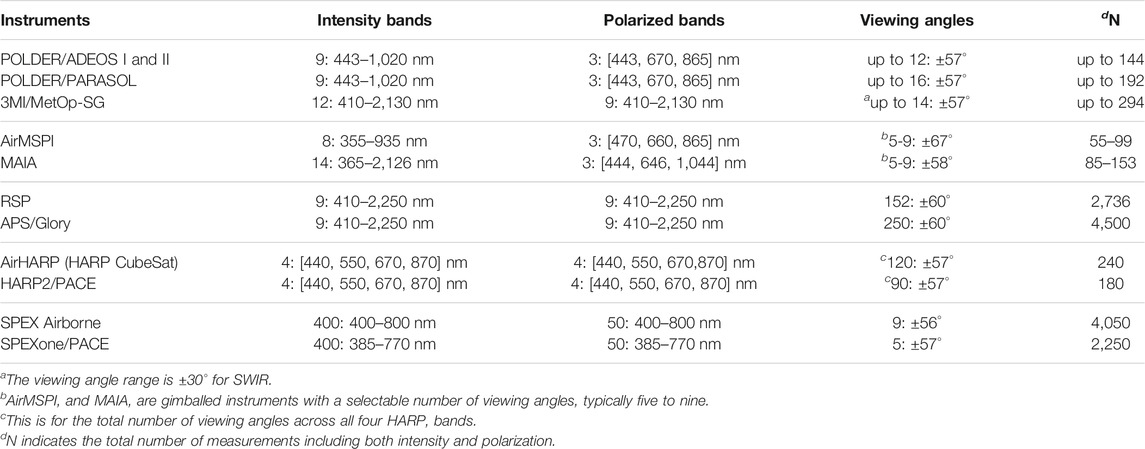
TABLE 1. The number and range of the spectral bands and view angles for various MAP instruments.

Extensive research has studied how aerosol retrieval uncertainties depend on the viewing angles available from MAP measurements. Hasekamp and Landgraf (2007) discussed the trade-off between spectral sampling and the number of viewing angles using synthetic data with spectral bands similar to POLDER, and found that the retrieval errors of aerosol optical depth (AOD), refractive index, and size are only slightly affected when the number of viewing angles is increased at the cost of the number of spectral sampling points, as long as at least three viewing angles are available. Based on synthetic high accuracy RSP measurements with either SWIR bands included or not, Wu et al. (2015) found that five angles equally spaced between ±60° provide sufficient accuracy for aerosol property retrievals, with performance gradually saturating as more angles are added beyond that. Similarly, Xu et al. (2017) concluded from AirMSPI measurements that the retrieval accuracy of AOD and single scattering albedo (SSA) do not improve significantly when more than around five viewing angles are used.

Although five viewing angles are sufficient for aerosol studies, in practice there will be ground pixels for which not all angles are optimal for aerosol retrievals due to impacts by cloud, sunglint, calibration artifacts, etc. Gao et al. (2019) used RSP measurements from the Ship-Aircraft Bio-Optical Research (SABOR) field campaign and found that viewing angles impacted by cloud needed to be removed in order to obtain high-quality retrieval results. Gao et al. (2021) found that AirHARP pixels impacted by cirrus clouds during the Aerosol Characterization from Polarimeter and Lidar (ACEPOL) field campaign produced large retrieval cost function values, indicative of larger deviation between the forward radiative transfer model and the measurements. Further, strong sunglint signals measured by both RSP and AirHARP instruments could not be modeled sufficiently well by the isotropic Cox and Munk (1954) model (Gao et al., 2019, 2021). Therefore, it is likely the number of suitable viewing angles for a given scene will be lower than those acquired by the sensor. The abundant angular measurements from the HARP instruments are useful to explore data quality screening by removing potentially problematic angles while maintaining sufficient useful angles for retrievals.

Due to their frequent presence, clouds are one of the major factors reducing the number of suitable viewing angles from multi-angular measurements (whether polarized or not) for aerosol studies. The MAP often observes a maximum angular range of 110–120° (Table 1). Depending on the size and height of a cloud, it may obscure Earth from all view angles or only over a small angular range. To address the challenges in the aerosol retrieval with cloud present, three approaches are often taken:

1. Completely remove the pixels influenced by clouds, using a cloud mask before (e.g. Garay et al. (2020)) and/or additional filtering after (Stap et al., 2015; Chen et al., 2020) the retrieval.

2. Simultaneous cloud and aerosol retrievals. This assumes an optically thin cloud covers most of the region in the observation, or a mixing of cloudy and clear sky pixels (Hasekamp, 2010; Stap et al., 2016).

3. For partially cloud-covered pixels, the angles impacted by cloud can be removed, and then a retrieval assuming only the presence of aerosols can be conducted (Gao et al., 2019).

For a pixel with most or all of its angles covered by cloud the retrieval can be either discarded (approach 1), or have both cloud and aerosol properties included in the state vector (approach 2). However, for a partially cloudy scene, there are open questions as to whether cloud-influenced angles can be removed effectively, and how much removal is practical before retrieval performance is degraded. In this study we focus on approach 3) and aim to answer the following three questions:

1. How many angles are sufficient in order to retrieve aerosol properties and ocean water leaving reflectance from HARP instruments with sufficient accuracy?

2. How can view angles problematic for aerosol retrievals, such as those influenced by clouds, be efficiently identified and removed (screened)?

3. How does the data screening improve the performance of aerosol and ocean color retrievals?

To understand to what extent the aerosol retrievals are still valid, we will examine the impact of the number of viewing angles on retrieval uncertainties using synthetic data simulated for both AirHARP and HARP2, which have different polarimetric uncertainties. The impacts of the scattering angle range will also be considered.

To identify the pixels impacted by water clouds, Stap et al. (2015) proposed using the retrieval cost function, a goodness-of-fit statistic based on how well the retrieval solution matches the observed measurements. Pixels whose cost function exceeded a threshold were deemed cloud-contaminated, and the whole pixel then discarded (approach 1 above). Building on this, we evaluate the fitting residuals (difference between the forward model and measurement) at each view angle. We implement a multi-angle polarimetric data screening (MAPDS) approach using these residuals as a metric to evaluate data quality, built upon the Fast Multi-Angular Polarimetric Ocean coLor (FastMAPOL) retrieval algorithm (Gao et al., 2021). FastMAPOL provides an efficient way to conduct aerosol and ocean color retrievals using efficient neural network (NN) forward models, while the data screening approach can automatically and adaptively identify and remove observations at view angles that cannot be well-represented by the forward model. Using AirHARP data, we will demonstrate the effectiveness of the data screening and how retrieval uncertainty changes after a portion of angles are removed.

MAPDS requires extra retrieval iterations and therefore slows down the retrieval. Retrieval speed can be improved using the neural networks for MAP measurements in both inverse model (Di Noia et al., 2015; Di Noia and Hasekamp, 2018), as well as forward models for ocean reflectance (Fan et al., 2019; Mukherjee et al., 2020) and coupled atmosphere and ocean model models (Gao et al., 2021). Another way to compensate for the increased computational cost, and also improve the overall FastMAPOL retrieval speed, is to improve the calculation of the Jacobian matrix that guides retrieval to a solution. This is challenging in MAP inversions due to the large number of retrieval parameters. To expedite the calculation, linearized radiative transfer models based on forward-adjoint perturbation theory have been developed (Spurr, 2008; Schepers et al., 2014). However, the linearization of the radiative transfer code requires sophisticated algorithm development. Instead, we employ automatic differentiation (AD) based on the NN forward model that acts as our radiative transfer (RT) emulator (Gao et al., 2021). AD Jacobians are based on the chain rule of derivatives (Baydin et al., 2018) and successfully reduce computational expense.

NASA’s PACE mission includes a hyperspectral scanning radiometer named the Ocean Color Instrument (OCI) and the two above-mentioned MAPs: HARP2 and SPEXone (Werdell et al., 2019). Together they will collect a large amount of multi-angle, hyperspectral, polarimetric measurements essential for the characterization of atmosphere and ocean states (Remer et al., 2019a,b; Frouin et al., 2019). To facilitate cross-calibration and data synergy, the measurements from all three PACE instruments will be projected onto a common PACE Level-1C data format with a uniform spatial grid. Aerosol and ocean color retrievals based on multiple instruments, with larger data volume, require even higher computational efficiency. The combination of FastMAPOL and data screening provide an efficient approach to analyze and process the large volume of measurements from PACE, either from one instrument or in combinations with others.

The impacts of ocean color retrievals from data screening will be also discussed in this study. To derive ocean color signals from the MAP measurement, we conducted atmospheric correction by subtracting the contributions of the atmosphere and ocean surface from the spaceborne or airborne measurements taken at the top of atmosphere (TOA) (Mobley et al., 2016). Note that for non-polarimetric ocean color sensors, neural networks trained on simulated TOA reflectance have been developed to conduct atmospheric correction. For example, the case 2 Regional Coast Colour (C2RCC) algorithm has been applied on ESA’s MEdium Resolution Imaging Spectrometer (MERIS) measurements (Doerffer and Schiller, 2007), and the Ocean Color - Simultaneous Marine and Aerosol Retrieval Tool (OC-SMART) algorithm has been applied on NASA’s Moderate Resolution Imaging Spectroradiometer (MODIS) measurements (Fan et al., 2021). In this study, neural networks are trained to represent the radiative transfer forward model over coupled atmosphere and ocean system which is used in the inversions of both aerosol and ocean parameters (Gao et al., 2021). The retrieved aerosol microphysical properties are then used to conduct the atmospheric correction on the multi-angle measurements. This procedure also allows the application of the MAP retrieved aerosol properties to atmospheric correction of co-located hyperspectral measurements from other sensors, such as PACE OCI (Gao et al., 2020; Hannadige et al., 2021).

This paper is organized as follow: Section 2 provides the methodology including the retrieval algorithm, NN forward model and AD Jacobian matrix; Section 3 describes synthetic HARP2 and AirHARP data retrievals to address question 1); Section 4 covers AirHARP filed data retrievals which address question 2) and 3); Section 5 discusses cloud mask and uncertainty analysis; Section 6 is the conclusions.

2 Methodology

2.1 Aerosol and Ocean Color Retrieval Algorithm

This study is based upon the efficient aerosol and ocean color retrieval algorithm FastMAPOL (Gao et al., 2021), which uses a NN forward model to conduct vector radiative transfer calculations for a coupled atmosphere and ocean system (Zhai et al., 2009, 2010). The forward model assumes a three-layer atmosphere: the bottom layer from ocean surface to an altitude of 2 km containing aerosols and molecules, a molecular layer between 2 km and the aircraft (at 20 km), and an additional molecular layer above the aircraft.

A total of 15 parameters are used in the forward radiative transfer simulation, as listed in Table 4 (more details in Gao et al. (2021)). The aerosol optical properties are determined by the fine and coarse mode complex refractive indices (total 4 parameters), and the volume densities (μm³μm⁻²) for five aerosol size submodes with each submode following a log-normal distribution. The mean radii and variances of the submodes are prescribed and fixed in the retrieval. The three smaller submodes in combination represent the fine mode, and the two larger submodes in combination represent the coarse mode. In this study we only consider open ocean waters modeled as a uniform layer with its bio-optical properties parameterized in terms of the chlorophyll-a concentration (Chla, $mg\cdot m^{-3}\left.\right)$ (Gao et al., 2019). Complex water properties over coastal water require additional parameters in the bio-optical model (Gao et al., 2018) which is subject to future investigations. The ocean surface roughness is represented by the isotropic model parameterized by wind speed (ms⁻¹) (Cox and Munk, 1954). As mentioned in Section 1, the sunglint signal measured by AirHARP can not be modeled well by the isotropic Cox and Munk model. In addition, it is challenging to accurately represent sunglint in the NN training due to its large amplitude in comparison with non-glint angles (Gao et al., 2021). To minimize the impacts of the sunglint, we limited the wind speed within 10 ms⁻¹ and excluded the view angles within 40° from the direction of specular reflection for the analysis in the next section. Larger wind speed and the associated white cap will be considered in future studies. Therefore, total 11 parameters are retrieved by FastMAPOL; the other four parameters needed by the forward model (viewing and solar zenith angle, relative azimuth angle, and ozone profile) are assumed to be known.

FastMAPOL determines optimal values of state parameters by minimizing the difference between the measurements and the NN forward model prediction. An iterative optimization approach is used as summarized in Figure 1A. The NN forward model computes the reflectance and degree of linear polarization (DoLP), defined as.

$\begin{array}{ccc}\hfill {\rho }_t& =\hfill & \frac{\pi L_t}{{\mu }_0{F}_0},\hfill \end{array}(1)$

$\begin{array}{ccc}\hfill P_t& =\hfill & \frac{\sqrt{Q_t^2+U_t^2}}{L_t},\hfill \end{array}(2)$

where L_t, Q_t, and U_t are the Stokes parameters at the sensor altitude, F₀ is the extraterrestrial solar irradiance, μ₀ is the cosine of the solar zenith angle. The differences between measurements and model predictions are represented by a cost function χ² based on Bayesian theory (Rodgers, 2000):

${\chi }^2\left(\mathbf{x}\right)=\frac{1}{N}\sum _i\left(\frac{{[{\rho }_t(i)-{\rho }_t^f(\mathbf{x};i)]}^2}{{\sigma }_{\rho }^2(i)}+\frac{{[P_t(i)-P_t^f(\mathbf{x};i)]}^2}{{\sigma }_P^2(i)}\right)(3)$

where ${\rho }_t^f$ and $P_t^f$ are the reflectance and DoLP computed from the NN forward model. The state vector x contains the forward-modeled parameters described above; the subscript i stands for the index of the measurements (where one “measurement” is defined as a pair of reflectance and DoLP) at different viewing angles and wavelengths; and N is the total number of measurements used in the retrieval. The maximum possible N assuming all angles are available is summarized for various MAPs in Table 1, which is 240 for AirHARP and HARP CubeSat, and 180 for HARP2.

FIGURE 1

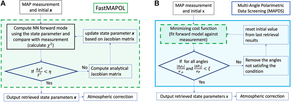
FIGURE 1. Flowcharts for (A) FastMAPOL retrievals and (B) retrievals with the multi-angle polarimetric data screening (MAPDS). In panel (A), $\mathrm{\Delta }{\chi }^2=|{\chi }_i^2-{\chi }_{i-1}^2|$ indicates the changes of the cost function between two iterations with η as threshold (Eq. 6). In panel (B), Δρ_t and ΔP_t indicate the difference between forward model and measurements for reflectance and DoLP with ξ as threshold (Eq. 8). The dashed box in (B) represents the same retrieval process as shown in the dashed box in (A). A maximum three passes (indicated by the loop in (B)) are used in the data screening process.

The total uncertainties of the reflectance and DoLP used in the algorithm are denoted by σ_ρ and σ_P, respectively. These include contributions from the instrument uncertainties σ_ins, the NN forward model uncertainties σ_NN, and the radiative transfer simulation uncertainties σ_RT used to train the NN:

$\begin{array}{ccc}\hfill {\sigma }_{\rho }^2& =\hfill & {\sigma }_{\rho ,ins}^2+{\sigma }_{\rho ,NN}^2+{\sigma }_{\rho ,RT}^2\hfill \end{array}(4)$

$\begin{array}{ccc}\hfill {\sigma }_P^2& =\hfill & {\sigma }_{P,ins}^2+{\sigma }_{P,NN}^2+{\sigma }_{P,RT}^2\hfill \end{array}(5)$

Table 2 summarizes the uncertainties used in this study; the values of σ_ρ,NN and σ_ρ,RT were determined in Gao et al. (2021) with the same NN models as used in this study. Note that, at present, uncertainties are assumed spectrally and angularly uncorrelated.

TABLE 2

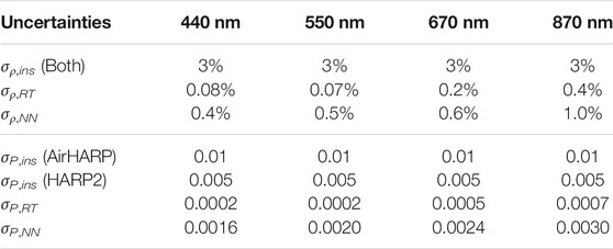
TABLE 2. Uncertainties for reflectance (ρ) and DoLP (P) for both measurement and forward model used in this study including instrument uncertainty (σ_ins), the radiative transfer simulation uncertainty (σ_RT), and the NN uncertainty (σ_NN). Different σ_P,ins is used for AirHARP and HARP2 but with the same σ_ρ,ins.

The FastMAPOL retrieval follows the flow chart in Figure 1A. In each iteration, if χ² is larger than a threshold, the state parameter x is updated to compute both ${\rho }_t^f$ and $P_t^f$, and a new value of cost will be computed. The Jacobian matrix (the gradient of the cost function with respect to $\mathbf{x}\left.\right)$) is used to determine the magnitude and direction for the updated estimate of x. This process iterates until the convergence criterion is met:

$\frac{|{\chi }_i^2-{\chi }_{i-1}^2|}{{\chi }_i^2}<\eta (6)$

where i is the iteration index in optimization, and ϵ is the convergence tolerance, taken as 0.01 in this study.

The convergence of the retrievals can be examined by the cost function histogram over an ensemble of retrievals (more discussion in the next section). If the retrievals converge well, the normalized cost function histogram can be represented by the theoretical probability density function (PDF) of the χ² distribution:

$f({\chi }^2,k)=\frac{{({\chi }^2)}^{k/2-1}{k}^{k/2}{e}^{-{\chi }^{2}k/2}}{2^{k/2}\mathrm{\Gamma }(k/2)}(7)$

where χ² is the cost function (Eq. 3), k is the degree of freedom (DOF), Γ(k/2) denotes the gamma function (James, 2006). The PDF is useful in understanding the behavior of the retrieval cost function distributions with different numbers of measurements used. After neglecting potential correlation between measurement uncertainties, we can approximate the DOF by the total number of measurements N, which shows good representation as demonstrated in the next section. Note that the DOF refers to the retrieval residuals in the cost function (Eq. 3), which are mostly contributed by the noise and uncertainties in the measurements and forward model. The DOF is likely between N and N-11, where 11 is the total number of retrieval parameters. The actual number of DOF can be determined from the Jacobian matrix and error covariance matrix (Rodgers, 2000).

2.2 Adaptive Data Screening

Based on the FastMAPOL retrieval algorithm, the MAPDS data screening approach, which conducts automatic data quality analysis and data screening, is summarized in the flowchart of Figure 1B. After each converged FastMAPOL retrieval, the residuals between each measurement and the forward model prediction are used to evaluate the data quality under the criteria:

$\frac{|\mathrm{\Delta }{\rho }_t|}{{\sigma }_{\rho }}<\xi ,\frac{|\mathrm{\Delta }{P}_t|}{{\sigma }_P}<\xi (8)$

where the residuals are compared with the uncertainty model defined in the cost function of Eq. 3, and ξ is a threshold. When either the reflectance or DoLP does not satisfy the criteria, the corresponding measurement is excluded from the cost function calculation (i.e., the view angle which cannot be represented well by the forward model is removed), and a new FastMAPOL retrieval is performed. In practice, additional screening rules based on the criteria may be used depending on the data quality of the field measurements (illustrated with an example later in Section 4). This process is repeated until all angles remaining satisfy Eq. 8. Note that the whole data screening process will include several retrieval passes, each involving multiple iterations until convergence. At the end of each retrieval pass based on the new forward model fittings, all measurements used in the retrieval are evaluated through Eq. 8 and subsequently excluded from the next round if they failed to pass. The data screening approach is an adaptive process, since it depends on the fitting at each iteration for each pixel. A threshold value of ξ = 3 is used in this study, which can be further tuned when more data is available. We found at most three passes of retrievals are sufficient to remove most of the problematic angles. Since the retrieved parameters from last retrieval can be used as the initial values to the next retrieval as shown in Figure 1, the total speed to conduct data screening are usually less than three times of the single round retrieval.

2.3 The NN Forward Model and Automatic Differentiation

The MAP retrievals are often computationally expensive due to their high dimensionality and iterative nature, with multiple forward model and Jacobian calculations. The data screening approach developed here further increases the demand for CPU computations because the retrieval must be repeated several times. Therefore, fast forward model and Jacobian matrix calculations are advantageous for efficient processing, which was a motivation for the use of NN forward models for AirHARP in (Gao et al., 2021). In this work we further improve the efficiency through automatic differentiation to compute the Jacobian matrix analytically (as opposed to numerically through finite differencing), exploiting the differentiable properties of the NN models.

The NN forward model developed in Gao et al. (2021) is a feed-forward neural network as defined in Table 3, where h₀ = x is the input layer that contains all 15 forward model parameters. Two sets of weight matrix W_p+1 and bias vector b_p+1 have been determined from the NN training process for reflectance and DoLP respectively (Gao et al., 2021), both with three hidden layers (k = 3) of 1,024, 256 and 128 nodes. Correspondingly, y is the output layer for either reflectance or DoLP at the four AirHARP bands.

TABLE 3

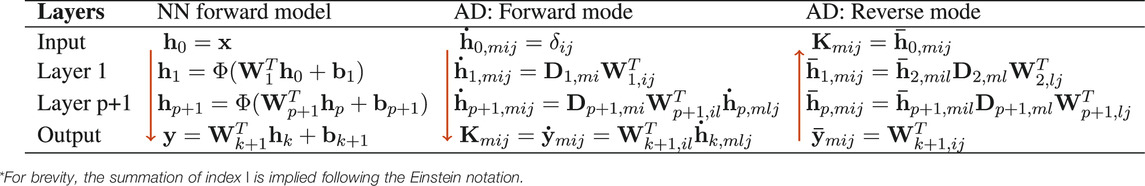
TABLE 3. NN forward model and its Jacobian matrix computed by the forward mode and reverse mode of automatic differentiation (AD). The arrows indicate the order of steps for each process.

For application to multi-angle measurements, the NN needs to be called to simulate y for each set of viewing and solar geometries for the state vector x. Elements of the Jacobian matrix are defined as follows:

${\mathbf{K}}_{mij}=\frac{\partial {\mathbf{y}}_{mi}}{\partial {\mathbf{x}}_{mj}}(9)$

Here index m indicates the viewing and solar angles, index i indicates the wavelength, and index j indicates the state parameter. Table 3 illustrates the structure of the NN and how the Jacobian matrix is calculated based on the trained weights. In that table, the nonlinear activation function Φ is the LeakyReLU function, which is defined as

$\mathrm{\Phi }{(\mathbf{Z})}_{mi}=\mathit{max}(0,{\mathbf{Z}}_{mi})+\alpha \times \mathit{min}(0,{\mathbf{Z}}_{mi}).(10)$

where α = 0.01, and Z is a matrix with m and i as its indices. The derivative with respect to each element in Φ is defined:

${\mathbf{D}}_{mi}=\frac{\partial \mathrm{\Phi }{(\mathbf{Z})}_{mi}}{{\partial \mathbf{Z}}_{mi}}=\left\{\begin{array}{c}1\text{\hspace{0.17em}\hspace{0.17em}if\hspace{0.17em}\hspace{0.17em}}{\mathbf{Z}}_{mi}>0\hfill \\ \alpha \text{\hspace{0.17em}\hspace{0.17em}if\hspace{0.17em}\hspace{0.17em}}{\mathbf{Z}}_{mi}<0\hfill \end{array}\right.(11)$

The finite difference (FD) method was used to compute the Jacobian matrix in FastMAPOL in (Gao et al., 2021), where the NN forward model was called twice per input parameter under the central difference approximation of derivatives. To reduce the computational cost, the Jacobian matrix can be derived analytically from the NN forward model using AD based on the chain rule of differentiation (Baydin et al., 2018). Two recursive relations are obtained to compute the Jacobian matrix as shown in Table 3, where the forward mode indicates the evaluation sequence from the first layer to the last layer, and the reverse mode indicates the evaluation sequence from the last layer to the first layer. To represent the recursive relations, we define ${\dot{\mathbf{h}}}_p$ (tangent) and ${\bar{\mathbf{h}}}_p$ (adjoint) as follows:

$\begin{array}{ccc}\hfill {\dot{\mathbf{h}}}_{p,mij}& =\hfill & \frac{\partial {\mathbf{h}}_{p,mi}}{\partial {\mathbf{x}}_{mj}},\hfill \end{array}(12)$

$\begin{array}{ccc}\hfill {\bar{\mathbf{h}}}_{p,mij}& =\hfill & \frac{\partial {\mathbf{y}}_{mi}}{\partial {\mathbf{h}}_{p,mj}}\hfill \end{array}(13)$

Note that h is defined in Table 3 (left column) as the output from each hidden layer of the NN. The Jacobian matrix can be represented by AD with either the tangent or the adjoint forms as the last step in Table 3:

$\begin{array}{ccc}\hfill {\mathbf{K}}_{mij}& =\hfill & {\dot{\mathbf{y}}}_{mij},\hfill \end{array}(14)$

$\begin{array}{ccc}\hfill {\mathbf{K}}_{mij}& =\hfill & {\bar{\mathbf{h}}}_{0,mij},\hfill \end{array}(15)$

where Eqs. 14, 15 are computed from the forward and reverse mode AD, respectively. Forward and reverse AD produce identical results, but differ in computational efficiency due to the different sequence of matrix operations and NN architecture. For optimal efficiency, we implemented AD directly based on the formalism summarized in Table 3 using the Pytorch library (Paszke et al., 2019). The arrows in the table indicate the order of calculation steps. NN forward model can be computed layer by layer, with the output from the previous layer as the input to the next layer. The forward mode AD can be computed in the same sequence as the NN forward model as shown in Table 3. The reverse mode AD is computed from the last layer backward to the first layer. Note that AD in both modes requires the values of matrix D as defined in Eq. 11, which is determined by the output of the NN forward model at each layer.

For the NN used in this study, AD in reverse mode provides the highest efficiency as investigated further in the next section. The AD methods are efficient and accurate in computing the Jacobian matrix, providing a convenient way to accelerate algorithms like FastMAPOL with a large number of retrieval parameters, making them more suitable for practical applications.

3 Synthetic AirHARP and HARP2 Data Retrievals

3.1 Synthetic Data

We performed radiative transfer simulations to generate 1,000 sets of synthetic polarized reflectances for a coupled atmosphere and ocean system as discussed in Section 2 and Gao et al. (2021). Here, we use a fixed solar zenith angle of 50° as this is approximately the solar zenith angle in the AirHARP field campaign data used in Section 4. Input parameters and their range are listed in Table 4; Chla is randomly sampled from a log-uniform distribution, AOD at 550 nm is sampled uniformly within [0,0.5], and the fine-mode volume fraction is sampled uniformly within [0, 1]. All the other parameters in Table 4 are sampled uniformly, except aerosol volume densities (which are determined by AOD and fine mode volume fraction). Simulations are performed with a view angle sampling of 1°. Random noise is added to the measurement according to the instrument uncertainties shown in Table 2.

TABLE 4

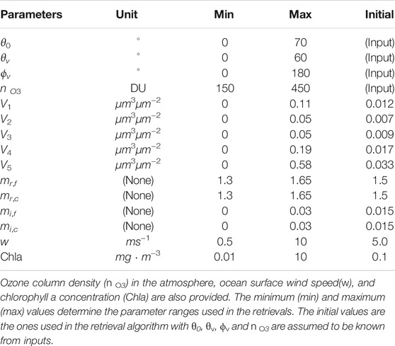
TABLE 4. Parameters used to represent the radiative transfer of the atmosphere and ocean system. θ₀ and θ_v are the solar and viewing zenith angles. ϕ_v is the relative viewing azimuth angle. V_i denote the volume densities for the five aerosol submodes. m_r and m_i are the real and imaginary parts of the refractive index. Subscripts f and c refer to fine and coarse mode.

In order to generate realistic viewing geometries we represent the orbit geometry as shown in Figure 2, where the viewing angles (θ_v, ϕ_v) can be sampled according to the along-track and cross-track angles indicated in the figure.

$\begin{array}{ccc}\hfill \tan {\varphi }_v& =\hfill & \frac{\tan {\theta }_c}{\tan {\theta }_a},\hfill \end{array}(16)$

$\begin{array}{ccc}\hfill \tan {\theta }_v& =\hfill & \frac{\tan {\theta }_c}{\cos {\varphi }_v},\hfill \end{array}(17)$

where θ_a and θ_c are the along-track and cross-track viewing angles. We use a set of predefined θ_a values (120 angles for AirHARP, 90 for HARP2) and then randomly sampled θ_c within ±47° according to HARP instrument characteristics. The resulting example geometries are shown in Figure 3A. Sunglint with view angles within a conservative angle of 40° relative to the direction of specular reflection are excluded as indicated in Figure 3. The simulated reflectance and DoLP are interpolated into this viewing geometry, each with a random value of θ_c. Note that Figure 2 is a simplified PACE orbit geometry with the solar azimuth angle in the along-track direction; the curvature of Earth’s surface is neglected.

FIGURE 2

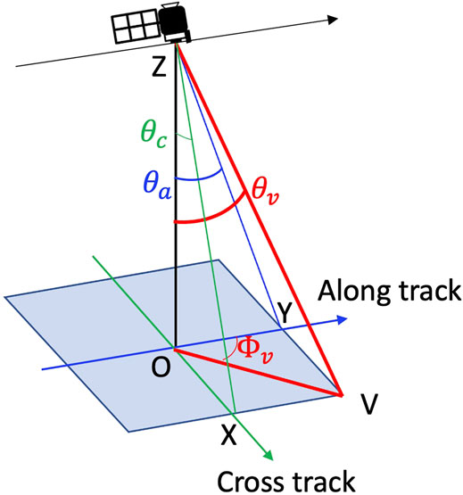
FIGURE 2. The observing geometry of the instrument at Z. The direction to an arbitrary location on the ground V can be determined by the along-track (OX direction) zenith angles θ_a, and the cross-track (OY direction) zenith angle θ_c. The viewing zenith and azimuth angles (θ_v, ϕ_v) can be derived through θ_a and θ_c as shown in Eqs 16, 17.

FIGURE 3

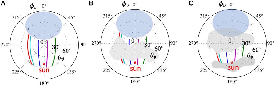
FIGURE 3. The sampled viewing directions (θ_v, ϕ_v) in the polar plot (four examples are shown with different color lines): (A) with all angles after excluding sunglint (the blue oval); (B) cloud blocking the central region; (C) cloud blocking both sides. When the cloud sizes are smaller enough, both b) and c) approach to (A). The asterisk indicate the antisolar point.

To evaluate the retrieval uncertainties using different numbers of viewing angles, we reduce the number of available viewing angles by assuming the MAP measurements are blocked randomly by clouds. Two cloud configuration schemes are considered:

1. Cloud blocking the center part of the measurements, leaving available angles on both sides. Cloud location can move randomly from one side to another side as shown in Figure 3B.

2. Clouds blocking both sides of the measurements, leaving the middle part of cloud-free angles available which can also move randomly from one side to another side as shown in Figure 3C.

We generate viewing geometries with the same total number of viewing angles (N_v) for both schemes as shown in Figures 3B,C. We chose 11 different cases with N_v of 5, 8, 10, 15, 20, 25, 30, 40, 50, 60, and 75 for AirHARP, and similarly for HARP2 with the two largest values as 56 and 58 instead. The largest averaged N_v value for both AirHARP and HARP2 corresponds to the case shown in Figure 3A with only sunglint removed and no cloud present. For the same number of N_v, Scheme 1 will result in a larger average range of scattering angles than Scheme 2. As shown in Table 1, the angular range of HARP2 and AirHARP measurements is 114°, therefore the cloud angular size (as viewed from ground) used to block the synthetic data can be estimated as 114° − N_v × 114°/90 for HARP2, and 114° − N_v × 114°/120 for AirHARP. Their physical size depends on both their angular size and height.

The retrievals are conducted for both AirHARP and HARP2 with their measurement uncertainties summarized in Table 2. This provides a total of 44,000 retrievals: 1,000 (RT simulation cases) × 2 (cloud schemes) × 2 (HARP2 and AirHARP) × 11 (total variations in angle number). Note that the total number of measurements N equals 10 for the case with N_v = 5, lower than the total 11 retrieval parameters, and therefore for that case the inverse problem is ill-posed with non-unique solutions.

3.2 Retrieval Efficiency Using FD and AD

The performance using FD with central difference is compared with the forward mode and reverse mode of AD as shown in Table 3 in Section 2. Figure 4 compares the retrieval χ² histogram and the retrieval time for the FD and AD methods. The results converge to similar χ² distributions; the χ² histograms change with respect to the available number of viewing angles, but can be well represented by the theoretical χ² distributions from Eq.7 with the same degree of freedom as the total number of measurements (N = 2N_v).

FIGURE 4

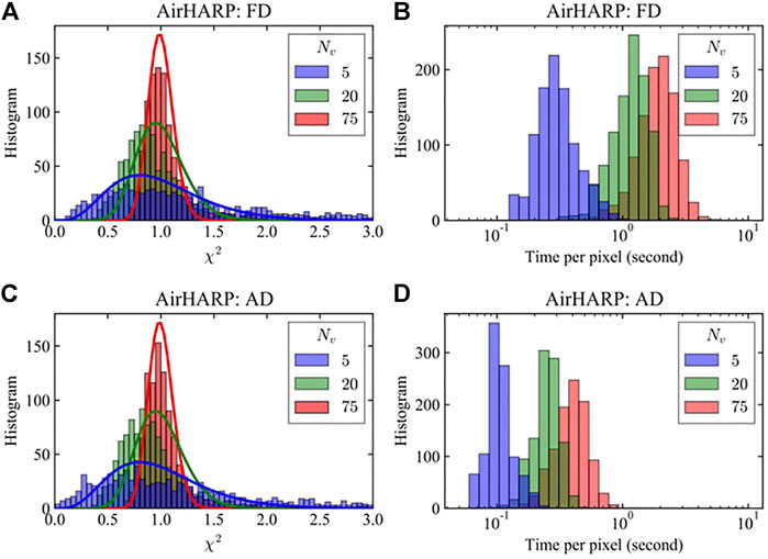
FIGURE 4. Histograms of χ² (A and C) and retrieval processing time (B and D) for synthetic retrievals and varying number of viewing angles (N_v) used. Solid lines in (A) and (C) indicate the χ² distributions with the appropriate DOF equal to the total number of measurements (2N_v). FD with central difference and AD with reverse mode are compared for both χ² and processing time. Viewing angles geometries are based on Figure 3C.

Retrievals using conventional radiative transfer simulation with FD usually took 1 hour to converge on a CPU (AMD EPYC Processor). Using neural network forward models, the averaged retrieval time decreased to 3 s using the same FD method and CPU. With forward and reverse modes of AD, a further decrease to 0.6 and 0.3 s respectively was achieved, which is an increase of speed by a factor of 5–10. With GPU processing (GeForce GTX 1060), the retrieval times were 0.08 and 0.05 s, another factor of 6 faster than CPU. AD in reverse mode provides the highest efficiency and will be used in the following discussions as the default method.

3.3 Aerosol Retrievals

In this section, we compare the retrieval error as a function of the number of available viewing angles. The retrieval error (except Chla), shown in Figure 5, is defined as the root mean square error (RMSE) between the retrieval results and the simulated truth. The retrieval error of Chla is represented by the Mean Averaged Error (MAE) in log scale which is a better metric for Chla as recommended by Seegers et al. (2018), and indicates the averaged ratio between the retrieval and truth values. The definition and performance of the retrieval error under different Chla range can be found in Gao et al. (2021). While it is well known that retrieval uncertainties depend on the aerosol loading (cf. Gao et al. (2021) for AirHARP data), for the convenience of discussion here, the retrieval errors are averaged over all cases with AOD within [0.01, 0.5]. The cloud blocking generally produces smaller errors than which has a smaller range of scattering angles. However, coarse mode v_eff seems less sensitive to the number of viewing angles and does not have a clear advantage between S1 and S2. Errors for HARP2 are also smaller than AirHARP due to the lower expected DoLP calibration uncertainty in HARP2.

FIGURE 5

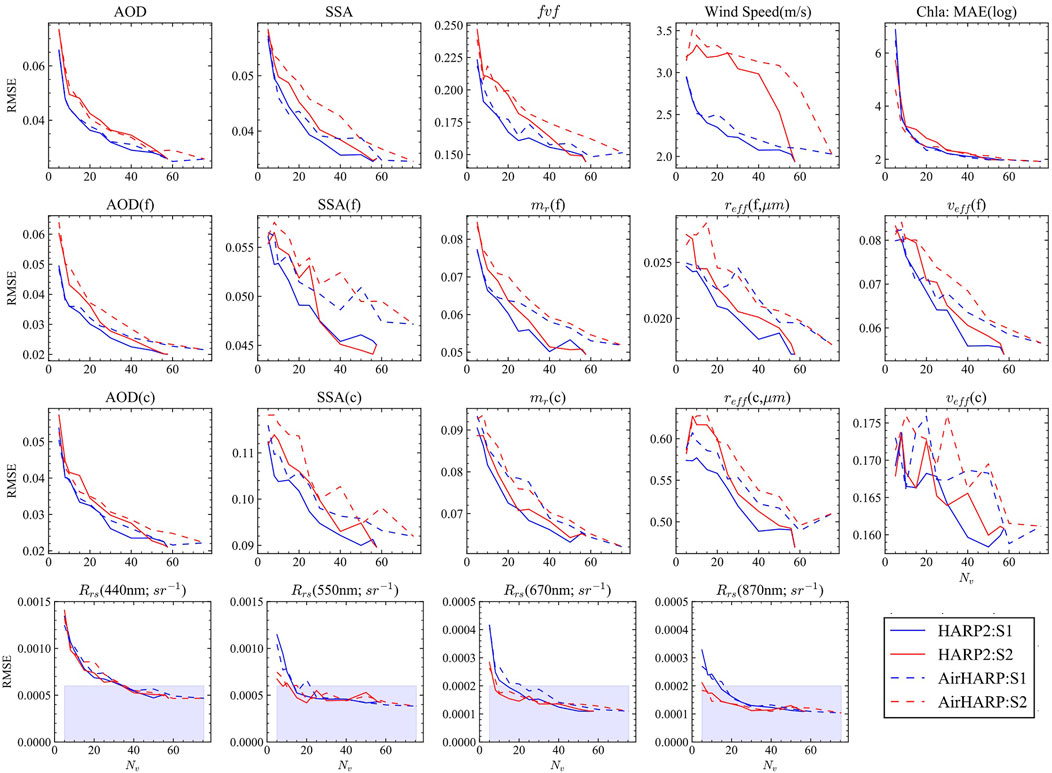
FIGURE 5. Retrieval errors in terms of root mean square error (RMSE) from the retrieval of 1,000 cases for AirHARP and HARP2, and with the two schemes of angle screening as shown in Figure 3. AOD and SSA RMSE are for the wavelength of 550 nm. Note that the retrieval errors for Chla is represented by the MAE error of Chla in log scale as used in Gao et al. (2021), which is different from other quantities. R_rs RMSE at all the four wavelengths with AOD (550 nm) $<0.2$ are shown in the last row with shaded area indicating the PACE mission R_rs uncertainty goal. The horizontal axis, N_v, is the total number of angles used in the retrievals, which is equivalent to the total number of unique measurements of 2N_v including both reflectance and DoLP across four HARP bands as discussed in Section 3.1.

Generally, the errors decrease rapidly as the total number of angles increases to 20 (corresponding to 2 × 20 unique measurements including both reflectance and DoLP across four HARP bands). For HARP2, improvement continues for AOD, SSA, m_r, r_eff, v_eff up to 40–50 angles; Chla performance seems to plateau around 20 angles. AOD error decreases the most, by a factor of three from 0.06 to 0.02. The total SSA error also decreases by a factor of two (from 0.06 to 0.03), but for modal (either fine or coarse mode) SSA and m_r, r_eff and v_eff, it only reduces by about 1/3 of its maximum error. Due to the removal of sunglint, the wind speed errors are relatively large with a value of 2–3 ms⁻¹. For AirHARP data, the decrease of the error is less pronounced due to the larger DoLP uncertainties of this sensor (Table 4), and 30 angles are generally needed, with marginal improvement after reaching 40 or more angles. Therefore a total 20–30 angles across all bands, i.e. five to eight viewing angles per band on average, seem sufficient to achieve good retrieval performance. As an example of having 30 continuous angles available for HARP2 measurements, the cloud angular size can be estimated to be 76° following the discussion in Section 3.1.

3.4 Remote Sensing Reflectance

The ocean signals are represented by the remote sensing reflectance, defined as the ratio between upwelling water-leaving radiance and the downwelling irradiance just above the ocean surface (Mobley et al., 2016). Through atmospheric correction, the remote sensing reflectance can be derived as:

$R_{rs}=\frac{({\rho }_t-{\rho }_{t,at{m}_{s}fc}^f)}{\pi }\left[\frac{C_{BRDF}}{T_d^{f,+}{t}_d^{f,+}}\right](18)$

where the reflectance contributed by the atmosphere and ocean surface $({\rho }_{atm+sfc}^f)$ and the transmittance and BRDF corrections ($C_{BRDF}/T_d^{f,+}{t}_u^{f,+}$) can be evaluated using the NN model in Gao et al. (2021) based on the retrieved aerosol and ocean properties. The viewing angle closest to nadir is used to compute R_rs.

Comparing the retrieved R_rs with the truth data computed from radiative transfer simulation with Sun at zenith and viewing angle at nadir, the last row in Figure 5 shows R_rs uncertainties in terms of RMSE for those simulations with AOD (550 nm) $<0.2$. Note that the R_rs uncertainties do not include the contribution from the additional random noise added in the synthetic data, therefore it is only used to represent the impacts from the aerosol and ocean surface property retrievals. For the application to PACE data, the calibration uncertainties for OCI is less than 0.5%, which can also be used to cross-calibrate PACE MAP measurements and therefore reduce the impacts of the MAP calibration uncertainties in R_rs evaluation. To achieve the PACE mission R_rs uncertainty goals (shown in Figure 5), the results suggest we need at least a total of 30 unique HARP angles for R_rs at 440 nm, approximately 10–20 angles for all other bands. With larger AOD in the range of [0.3,0.5], the errors increase up to 0.001 even when all angles are used (not shown) as accurate atmospheric correction becomes more challenging due to the increased signal from aerosols.

4 AirHARP Field Data Retrievals

The ACEPOL field campaign conducted aerosol and cloud measurements from the NASA high altitude ER-2 aircraft from October to November of 2017 over a variety of scenes including oceans, urban areas, intensive agriculture, forests and high desert around California, Nevada and Arizona (Knobelspiesse et al., 2020). The field campaign involved four MAP instruments including AirHARP, AirMSPI, SPEX airborne, and RSP (Table 1), as well as two lidar sensors–HSRL-2 (Burton et al., 2015) and CPL (the Cloud Physics Lidar) (McGill et al., 2002). Aerosol retrievals have been conducted based on the MAP measurements from ACEPOL (Fu et al., 2020; Gao et al., 2020; Puthukkudy et al., 2020; Gao et al., 2021; Hannadige et al., 2021). Simultaneous aerosol and ocean color retrievals have been performed over three AirHARP scenes (Gao et al., 2021). In this study we focus on AirHARP Scene where cirrus clouds were reported to impact the aerosol retrievals. A portion of AirHARP viewing angles impacted by the water condensation on the instrument front lens has been removed from the dataset.

The RGB images of AirHARP scene at three different viewing directions with θ_a = − 20°, 0°, 20° are shown in Figure 7A1–C1. Two cloud patches are indicated in Figure 6 as A and B. Due to the parallax effect (the data are geolocated to the surface while the clouds are elevated), A and B appear at different locations when viewed from the three angles. Since our data screening criteria are applied to each angle and wavelength combination, the approach is not affected by the data being geolocated to an altitude other than cloud top. As discussed in the next section, a multi-angle cloud mask can be developed based on data geolocated at the surface.

FIGURE 6

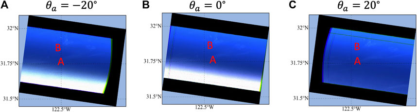
FIGURE 6. (A-C) RGB images of the AirHARP measurements at 10/23/2017 at three different along track viewing angles$\left({\theta }_a\right.=-20°,0°,20°$).Two cloud patches are indicated by A and B.

4.1 Adaptive Data Screening

To identify and remove cloud-affected view angles, we apply the data screening approach (MAPDS) as explained in Figure 1B. Figure 7 provides an example comparing the measurement and fitted reflectance and DoLP from one pixel near cloud A after the first pass of retrievals. Here σ_ρ and σ_P indicate the uncertainties used in the cost function, Δρ_t and ΔP_t indicate the residuals (difference between the forward model and measurements), and Δρ_t/σ_ρ and ΔP_t/σ_P the normalized residuals as used in the cost function (Eq. 3).

FIGURE 7

FIGURE 7. (A,B) Fitted reflectance and DoLP (circles) and AirHARP measurements (dots) for a pixel near cloud A after the first pass of retrievals; (C,D) uncertainty model as defined in Eqs 4 and 5; (E,F) fitting residuals; (G,H) normalized fitting residuals. The blue shaded region was identified by the data screening method as cloud-contaminated. Most DoLP measurements at 440 and 870 nm at viewing angles larger than 0° are also removed. Measurements within the red shaded region were removed due to water condensation on the instrument lens.

The blue shaded region was identified as cloud contaminated due to the relatively large ρ_t/σ_ρ at all bands (with the largest at 870 nm), and the large ΔP_t/σ_P, at the 670 nm band. As a further buffer, we removed any angles within 4° of angles screened by either reflectance or DoLP criteria at 550 or 670 nm bands. In this way, both reflectance and DoLP measurements in the blue shaded region are excluded. We chose 550 and 670 nm bands as reference based on their higher data quality comparing with other bands (Gao et al., 2021) which can be adjusted for application to other datasets. For 440 and 870 nm bands outside of the blue and red shaded region, the screening criteria from Eq. 8 are still applied independently for reflectance and DoLP, which results in mostly DoLP angles removed. The final retrieval (at the third retrieval pass) is done using the remaining measurements after data screening and resulted in a value of χ² reduced from 4.98 to 0.6, and the retrieved total AOD reduced from 0.064 to 0.052.

For the AirHARP data used in Gao et al. (2021), the measurement uncertainties were larger than expected at 440 and 870 nm. In that study, DoLP measurements from the 440 nm band were excluded manually. In this study, the adaptive screening approach is able to automatically identify and remove the problematic angles at 440 nm band, providing an automatic data quality control mechanism.

4.2 Retrieval Results

Figure 8 shows retrieval results with and without the adaptive data screening. As seen in Figure 8A1, the maximum number of total viewing angles is 120 around the center upper region. The elongated region with large χ² values in Figure 8C1 is due to the impacts of the cirrus cloud (Figure 7). Clouds can be viewed from a broader range of pixels in the along-track direction, which impacts the retrieval performance. The retrieved AOD at 550 nm in Figure 8D1 has a clear covariation with χ² with the highest AOD around clouds A and B. The R_rs at 550 nm are mostly smooth with small variations that seems to also relate to cloud patterns. Therefore, the maximum number of viewing angles for DoLP is around 100 as shown in Figure 8B1 (recall as discussed above DoLP at 440 nm was excluded from retrievals in Figure 8). Figure 8A2–E2 applied the criteria of N_v > 30 and χ² < 2 to ensure the retrieval quality, removing most of the pixels around the clouds due to the large χ² values and leaving an elongated holes in the retrieved AOD and R_rs.

FIGURE 8

FIGURE 8. Retrievals on the AirHARP scene over ocean without data screening (all angles, first and second columns) and with MAPDS (third and fourth columns). Panels show the number of viewing angles (N_v) for the reflectance (A1–A4) and DoLP (B1–B4), retrieval cost function $\left({\chi }^2\right.$, C1–C4), retrieved AOD (D1–D4) and retrieved $R_{rs}(s{r}^{-1}$, E1–D4). The first and third columns show all retrieved pixels; the second and the fourth columns show pixel satisfying criteria of N_v >30 and χ²<2, respectively. The HSRL AOD at 532 nm is indicated as colored dots in the AOD plots (D1–D4). Same as Figure 6, two cloud patches are indicated by A and B.

After applying the MAPDS screening process, the number of available angles around clouds are reduced (Figure 8A3, B3) and χ² (Figure 8C3) becomes much more uniform. Similarly, as seen in Figure 8D3, the prominent large AOD regions around points A and B are reduced. Most of the cirrus cloud features for R_rs from Figure 8E1 are removed as shown in Figure 8E3. There are still minor remaining artifacts for R_rs in Figure 8E3 which can be further reduced by choosing a smaller χ² threshold in the analysis. Note that the data screening process also removed some of the original viewing angles closest to nadir and the new R_rs can be computed using an angle further away which helps reduce the impacts of cirrus cloud on R_rs. Future improvement may require using multiple angles to analyze R_rs. After applying the criteria of N_v > 30 and χ² < 2 in Figure 8A4–E4, the pixels removed are mostly around the edge of the image due to the small number of available viewing angles. The N_v criterion is important to ensure a sufficient number of measurements used in the retrievals.

As shown in Figure 8D2, the criteria N_v > 30 and χ² < 2 result in many retrievals being discarded when all angles are used in the processing. After applying the data screening, the χ² are greatly reduced; this reduction in χ² outweighs the decrease in N_v, with the effect that most of these discarded retrievals are now retained (Figure 8D4). The valid retrieval pixels almost doubled after MAPDS. These pixels mostly have N_v larger than 50; synthetic retrievals in Figure 5 imply an AOD retrieval uncertainty of 0.03 for AOD up to 0.5. For smaller AOD around 0.1, the retrieval uncertainty can be as low as 0.01 (Gao et al., 2021).

The retrieved AirHARP AOD at 550 nm is compared with the HSRL AOD at 532 nm in Figure 9 for two lines (A1–A2) across point A, and (B1–B2) across point B. The mean and standard deviation after averaging 4 × 4 pixels (2.2 km × 2.2 km) areas are used in the comparison, and only pixels satisfying N_v > 30 and χ² < 2 are considered. To mitigate the influence from atmospheric turbulence in the field measurement, the HSRL AOD is estimated by multiplying an assumed lidar ratio of 40sr with the aerosol backscatter coefficient derived from the HSRL technique, and the corresponding AOD systematic uncertainty is estimated to be 50% (Fu et al., 2020). An additional cirrus cloud mask, which uses thresholds of backscatter ratio greater than 1 (backscatter ratio is the ratio of the particulate backscatter to molecular backscatter) and particulate depolarization greater than 0.2 above 8 km, has been applied on the HSRL-2 data. The AirHARP AOD fills in the data gaps due to the cirrus cloud mask between HSRL AOD results with a few overlapped pixels. The retrievals with all angles in Figure 9B1 show differences of 0.019 between the averaged AOD from AirHARP and HSRL, but after applying the data screening, these differences reduce to 0.005 in Figure 9B2. The averaged difference shown in (a1) and (a2) are similar to each other with a value of 0.01. However, a peak in Figure 9A1 with a magnitude of 0.17 is reduced to a value of 0.07 after the angles influenced by cloud are removed in Figure 9A2. Similarly, the peaks in Figure 9B1 with a value up to 0.15 is reduced to below 0.09 as shown in Figure 9B2.

FIGURE 9

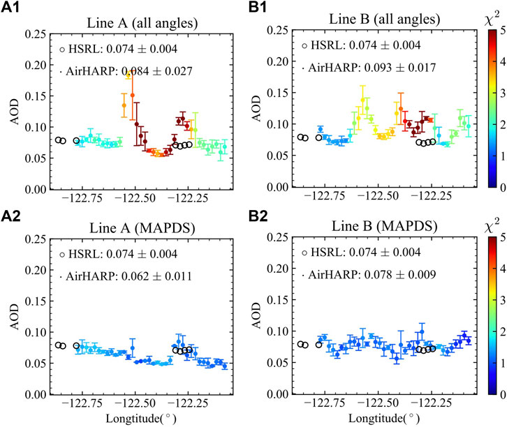
FIGURE 9. Mean (colored dots) and standard deviation (bars) of the retrieved AirHARP AOD at 550 nm averaged over 4×4 pixels (2.2km ×2.2 km) for two along track lines across cloud patch A (line A, A1–A2) and cloud patch B (line B, B1–B2). HSRL AODs at 532 nm are indicated by circles. For the retrieval results with all angles (A1–B1), most pixels converge into χ² values larger than 2, but for retrievals with MAPDS (A2–B2) most pixels converged within χ²<2. The χ² value for the corresponding AirHARP AODs are indicated by its color label in the plots.

However, there are small variations of the retrieved AOD in the vicinity of cloud locations, which may be related to light scattering from the 3D structure of cloud and/or aerosol humidification effects. The small inhomogeneity of R_rs near clouds may be due to the artifacts from the aerosol retrievals or the presence of cirrus clouds. The pixels which are influenced by the cirrus cloud can be identified from the remaining number of measurement angles (N_v).

5 Discussion

5.1 Retrieval Uncertainties and Cost Function

Retrieval uncertainties can be evaluated in two ways: 1) the truth-in and truth-out studies as for the synthetic data in Section 3, where the retrieval errors are evaluated by comparing the retrieval results with the truth data in the synthetic data; 2) Using error propagation based on the Jacobian matrix. The second method is effective to evaluate the retrieval uncertainties and have been used to study MAP measurements (Knobelspiesse et al., 2020) and more broadly in aerosol remote sensing (Sayer et al. (2020) for a review). However, it represents a best-case uncertainty, as it is based on various assumptions including that our knowledge on the uncertainty models in the cost function (Eq. 3) are accurate, that the retrievals converge to their global minimum, and that the forward model is close to linear near the solution (see Povey and Grainger (2015) for a review). Retrieval first guesses are important, as convergence to local minima when starting from different initial values can be a problem for high-dimensional retrievals (Gao et al., 2020)

The histogram of χ² for retrievals with all angles and with the adaptive screening are shown in Figure 10, with most probable values of 1.85 and 1.35 respectively. Because these values are larger than 1, the retrieval uncertainty budget for σ_ρ and σ_P (Table 2) may underestimate the real total uncertainties. The total number of reflectance and DoLP measurements used in the retrieval are 112 and 85 on average according to Figure 8A1, B1, and Figure 8A3, B3, respectively. The theoretical χ² distribution from Eq. 7 with degree of freedom of 85 can represent the histogram for MAPDS well after normalizing its most probable value to the same value of 1.35 as for the histogram. However, the width is slightly smaller, which may indicate overfitting of the data relating to the uncertainty correlation between angles. The retrieval results using all angles have a much wider distribution which cannot be approximated by theoretical χ² distribution. The fact that the histogram after adaptive screening matches the theoretical expectation more closely indicates that the rejected angles led to outliers as they did not fit the assumed forward model and (Gaussian) uncertainty assumption. To evaluate retrieval uncertainties using error propagation in future studies, the total uncertainties may need to be multiplied by a factor of 1.35 due to this cost mismatch. A further complication, not widely addressed in the remote sensing community, is that this work (and many others) assumes no spectral or angular correlation between measurement/forward model uncertainties, or between errors in nearby pixels. As discussed by Sayer et al. (2020), this has consequences in terms of uncertainty estimates and cost function when these correlations exist in the real world. However, these correlations are hard to incorporate into retrievals because their magnitudes are, in most cases, poorly known. The presence of correlations also complicates the theoretical χ² distribution, and a more complex generalized χ² distribution should ideally be used to determine optimal cost thresholds for data filtering, if correlations can be determined.

FIGURE 10

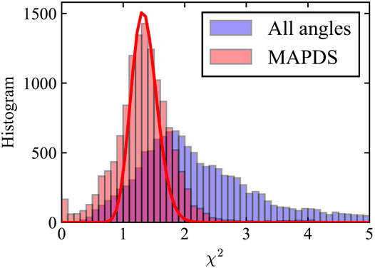
FIGURE 10. Histogram of the χ² for Figure 8 (C1) (with all angles) and (C2) (with MAPDS) with its most probable values of 1.85 and 1.35 respectively. The average number of measurements including both reflectance and DoLP used in the retrievals are 112 and 85 respectively. The theoretical curve (red line) is for 85 degrees of freedom, shifted to the same most probable value of 1.35 as the histogram.

5.2 MAPDS as a Multi-Angle Cirrus Cloud Mask

The RGB images in Figure 6 indicated two cloud patches, which can be identified and removed by MAPDS. In this sense the screening can serve as an angle-by-angle cloud mask for multi-angle data. Figure 11A1–C1 shows the reflectance at 670 nm for the same three viewing angles of Figure 6, and indicates the angles identified by MAPDS at 670 nm, which correspond to clouds A and B very well. The lengths for cloud A and B in the along-track direction are estimated to be around 5–8 km. The displacement between the cloud A locations in Figure 11A2, C2 is estimated through the cross correlation of the masked reflectance from Figure 11A2, C2 in the along-track lines, which shows a change of distance (Δd) of 7–9 km. With the angular span of 2 × 20°, the height of the cloud can be estimated as ctan (20°) ×Δd/2 which is 10–12 km. This assumes no significant cloud motion in the along-track direction during the time interval between the measurements at the two viewing directions. Note that we have assumed the cloud is not moving during the time interval when conducting measurements at the two viewing directions. A more precise treatment considering cloud motion may be conducted by involving more viewing angles at different observing times.

FIGURE 11

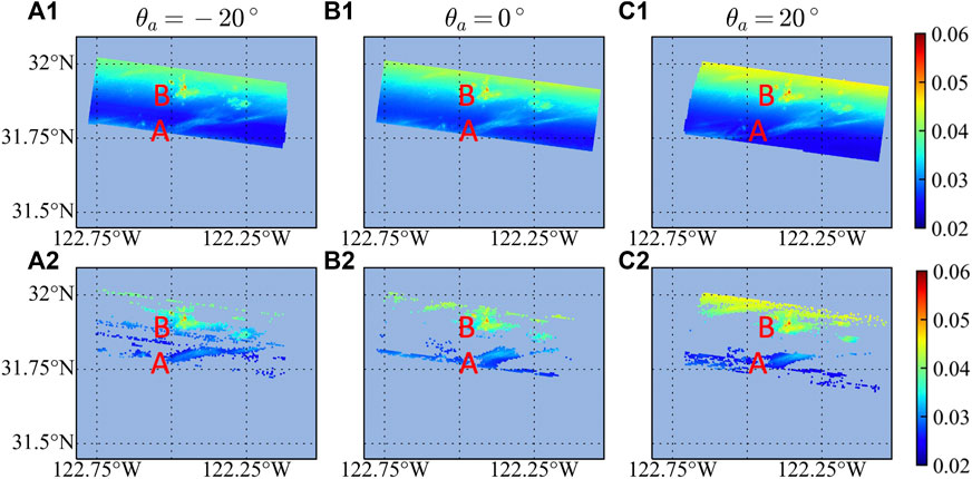
FIGURE 11. Same as Figure 6 but for the reflectance for the red (670 nm) band after sunglint angles are removed (A1–C1), and the identified cloudy pixels by MAPDS (A2–C2). Two cloud patches are indicated by A and B. The linear feature may be due to an artifact from water condensation on the instrument lens.

The screening could be used to generate a cloud fraction by dividing the number of viewing angles impacted by clouds by the total number of angles. For PACE, OCI’s viewing angle will be 20°, and SPEXone viewing angles include both ±20° viewing angles (and other three angles), therefore a HARP2-derived MAPDS cloud mask could be used to complement cloud masks generated by OCI and/or SPEXone. This possibility will be assessed in future studies when PACE data are available.

5.3 Data Quality Control

In this study, we discussed the removal of angles for the HARP measurements by filtering out view angles that are problematic for aerosol retrievals to improve data quality. Analogous concepts may be applied to other instruments, such as in the hyperspectral rather than angular domains for OCI and SPEXone. The removed measurements can also be used to identify instrument artifacts or cases involving excess amounts of sunglint due to insufficient information on wind direction, surface slopes, and other factors (Gao et al., 2019). The data with better-modeled glint characteristics can then be used for further analysis in simultaneous aerosol and glint retrievals (Knobelspiesse et al., 2021).

6 Conclusion

In this study we developed and analyzed a data thinning technique to improve performance of aerosol and ocean color retrievals from hyper-angular MAPs by screening and removing problematic measurements affected by cloud and other anomalies. We investigated the impact of the number of viewing angles on retrieval uncertainty for the AirHARP and HARP2 instruments based on synthetic data, finding that a total of 20–30 unique angles across all bands (five to eight viewing angles per band in average) were sufficient to achieve good retrieval performance. Therefore, the total number of viewing angles of HARP2 (90) and AirHARP (120) allows for some screening while retaining sufficient observations for high-quality retrievals.

We further developed and applied an automatic adaptive data screening approach called MAPDS to the AirHARP field measurements. We found that it effectively identified and removed angles influenced by thin cirrus clouds, increasing the level of agreement with independent AOD data from airborne HSRL-2, and providing an additional angle-by-angle cloud mask. We also found that this screening resulted in a better match of retrieval cost to theoretical χ² distributions. To improve processing efficiency and accuracy, deep learning techniques including neural network and automatic differentiation are explored. The FastMAPOL algorithm using neural network has demonstrated a factor of 1,000 speed improvement. After we replaced numerical calculation of Jacobians with automatic differentiation of the neural network forward model, the retrieval speed is improved by another factor of 10, more than compensating for the additional overhead of the screening process. The FastMAPOL algorithm and the adaptive screening approach provide efficient ways to process multi-angle polarimetric measurements for NASA’s Plankton, Aerosol, Cloud, ocean Ecosystem (PACE) mission, and can be applied to other modern remote sensing studies where a large amount of data collected.

Data Availability Statement

The AirHARP and HSRL-2 data used in this study are available from the ACEPOL data portal (https://doi.org/10.5067/SUBORBITAL/ACEPOL2017/DATA001, ACEPOL Science Team, 2017). The FastMAPOL retrieval results are available from NASA Open Data Portal without data screening (https://data.nasa.gov/Earth-Science/FastMAPOL_ACEPOL_AIRHARP_L2/8b9y-7rgh) and with data screening (https://data.nasa.gov/Earth-Science/MAPDS/tn52-gr4h).

Author Contributions

MG, KK, BF, and P-WZ formulated the original concept for this study. MG developed the algorithm and generated the scientific data. P-WZ developed the radiative transfer code used to train the NN model. KK, AS, and OH advised on the uncertainty analysis and cloud mask. BF, AI and P-WZ advised on the ocean products. KK, P-WZ, AS, BC and YH advised on the aerosol products. VM and XX provided and advised on the AirHARP data. RF, SB, and MF provided and advised on the HSRL-2 data. All authors provided critical feedback and contributed to the final manuscript.

Funding

MG, KK, BF, BC, AI, AS, and P-WZ have been supported by the NASA PACE project. P-W has been supported by NASA (grants 80NSSC18K0345 and 80NSSC20M0227). Funding for the ACEPOL field campaign came from NASA (ACE and CALIPSO missions) and SRON. Part of this work has been funded by the NWO/NSO project ACEPOL (project no. ALWGO/16-09). The ACEPOL campaign has been supported by the NASA Radiation Sciences Program.

Conflict of Interest

Author MG was employed by Science Systems and Applications, Inc.

The remaining authors declare that the research was conducted in the absence of any commercial or financial relationships that could be construed as a potential conflict of interest.

Publisher’s Note

All claims expressed in this article are solely those of the authors and do not necessarily represent those of their affiliated organizations, or those of the publisher, the editors and the reviewers. Any product that may be evaluated in this article, or claim that may be made by its manufacturer, is not guaranteed or endorsed by the publisher.

Acknowledgments

The authors would like to thank the ACEPOL science team for conducting the field campaign and HARP and HSRL teams for providing the data. We thank the NASA Ocean Biology Processing Group (OBPG) system team for supports in the high-performance computing (HPC). We appreciate the constructive discussions with Feng Xu, Jason Xuan and Sean Foley.

References

Baydin, A. G., Pearlmutter, B. A., Radul, A. A., and Siskind, J. M. (2018). Automatic Differentiation in Machine Learning: a Survey. J. Machine Learn. Res. 18, 1–43.

Google Scholar

Boucher, O., Randall, D., Artaxo, P., Bretherton, C., Feingold, G., Forster, P., et al. (2013). “Clouds and Aerosols,” in Climate Change 2013: The Physical Science Basis. Editors T. F. Stocker, D. Qin, G.-K. Plattner, M. Tignor, S. K. Allen, J. Boschunget al. (Cambridge, United Kingdom and New York, NY, USA): Cambridge University Press), 571–658. Contribution of Working Group Ito the Fifth Assessment Report of the Intergovernmental Panel on Climate Change. doi:10.1017/CBO9781107415324.016

CrossRef Full Text | Google Scholar

Burton, S. P., Hair, J. W., Kahnert, M., Ferrare, R. A., Hostetler, C. A., Cook, A. L., et al. (2015). Observations of the Spectral Dependence of Linear Particle Depolarization Ratio of Aerosols Using Nasa langley Airborne High Spectral Resolution Lidar. Atmos. Chem. Phys. 15, 13453–13473. doi:10.5194/acp-15-13453-2015

CrossRef Full Text | Google Scholar

Cairns, B., Russell, E. E., and Travis, L. D. (1999). Research Scanning Polarimeter: Calibration and Ground-Based Measurements. Proc.SPIE 3754, 186–196. doi:10.1117/12.366329

CrossRef Full Text | Google Scholar

Chen, C., Dubovik, O., Fuertes, D., Litvinov, P., Lapyonok, T., Lopatin, A., et al. (2020). Validation of Grasp Algorithm Product from Polder/parasol Data and Assessment of Multi-Angular Polarimetry Potential for Aerosol Monitoring. Earth Syst. Sci. Data 12, 3573–3620. doi:10.5194/essd-12-3573-2020

CrossRef Full Text | Google Scholar

Chowdhary, J., Cairns, B., Mishchenko, M., and Travis, L. (2001). Retrieval of Aerosol Properties over the Ocean Using Multispectral and Multiangle Photopolarimetric Measurements from the Research Scanning Polarimeter. Geophys. Res. Lett. 28, 243–246. doi:10.1029/2000GL011783

CrossRef Full Text | Google Scholar

Chowdhary, J., Cairns, B., Mishchenko, M. I., Hobbs, P. V., Cota, G. F., Redemann, J., et al. (2005). Retrieval of Aerosol Scattering and Absorption Properties from Photopolarimetric Observations over the Ocean during the Clams experiment. J. Atmos. Sci. 62, 1093–1117. doi:10.1175/JAS3389.1

CrossRef Full Text | Google Scholar

Cox, C., and Munk, W. (1954). Measurement of the Roughness of the Sea Surface from Photographs of the Sun's Glitter. J. Opt. Soc. Am. 44, 838–850. doi:10.1364/josa.44.000838

CrossRef Full Text | Google Scholar

Deschamps, P.-Y., Breon, F.-M., Leroy, M., Podaire, A., Bricaud, A., Buriez, J.-C., et al. (1994). The Polder mission: Instrument Characteristics and Scientific Objectives. IEEE Trans. Geosci. Remote Sens. 32, 598–615. doi:10.1109/36.297978

CrossRef Full Text | Google Scholar

Di Noia, A., and Hasekamp, O. P. (2018). Neural Networks and Support Vector Machines and Their Application to Aerosol and Cloud Remote Sensing: A Review. Cham: Springer International Publishing, 279–329. doi:10.1007/978-3-319-70796-9_4

CrossRef Full Text | Google Scholar

Di Noia, A., Hasekamp, O. P., van Harten, G., Rietjens, J. H. H., Smit, J. M., Snik, F., et al. (2015). Use of Neural Networks in Ground-Based Aerosol Retrievals from Multi-Angle Spectropolarimetric Observations. Atmos. Meas. Tech. 8, 281–299. doi:10.5194/amt-8-281-2015

CrossRef Full Text | Google Scholar

Diner, D. J., Boland, S. W., Brauer, M., Bruegge, C., Burke, K. A., Chipman, R., et al. (2018). Advances in Multiangle Satellite Remote Sensing of Speciated Airborne Particulate Matter and Association with Adverse Health Effects: from MISR to MAIA. J. Appl. Rem. Sens. 12, 1–22. doi:10.1117/1.JRS.12.042603

CrossRef Full Text | Google Scholar

Doerffer, R., and Schiller, H. (2007). The Meris Case 2 Water Algorithm. Int. J. Remote Sens. 28, 517–535. doi:10.1080/01431160600821127

CrossRef Full Text | Google Scholar

Dubovik, O., Li, Z., Mishchenko, M. I., Tanré, D., Karol, Y., Bojkov, B., et al. (2019). Polarimetric Remote Sensing of Atmospheric Aerosols: Instruments, Methodologies, Results, and Perspectives. J. Quant. Spectrosc. Radiat. Transfer 224, 474–511. doi:10.1016/j.jqsrt.2018.11.024

CrossRef Full Text | Google Scholar

Fan, C., Fu, G., Di Noia, A., Smit, M., Rietjens, J. H. H., Ferrare, R. A., et al. (2019). Use of a Neural Network-Based Ocean Body Radiative Transfer Model for Aerosol Retrievals from Multi-Angle Polarimetric Measurements. Remote Sens. 11, 2877. doi:10.3390/rs11232877

CrossRef Full Text | Google Scholar

Fan, Y., Li, W., Chen, N., Ahn, J.-H., Park, Y.-J., Kratzer, S., et al. (2021). Oc-smart: A Machine Learning Based Data Analysis Platform for Satellite Ocean Color Sensors. Remote Sens. Environ. 253, 112236. doi:10.1016/j.rse.2020.112236

CrossRef Full Text | Google Scholar

Fougnie, B., Marbach, T., Lacan, A., Lang, R., Schlüssel, P., Poli, G., et al. (2018). The Multi-Viewing Multi-Channel Multi-Polarisation Imager - Overview of the 3MI Polarimetric mission for Aerosol and Cloud Characterization. J. Quant. Spectrosc. Radiat. Transfer 219, 23–32. doi:10.1016/j.jqsrt.2018.07.008

CrossRef Full Text | Google Scholar

Frouin, R. J., Franz, B. A., Ibrahim, A., Knobelspiesse, K., Ahmad, Z., Cairns, B., et al. (2019). Atmospheric Correction of Satellite Ocean-Color Imagery during the Pace Era. Front. Earth Sci. 7, 145. doi:10.3389/feart.2019.00145

PubMed Abstract | CrossRef Full Text | Google Scholar

Fu, G., Hasekamp, O., Rietjens, J., Smit, M., Di Noia, A., Cairns, B., et al. (2020). Aerosol Retrievals from Different Polarimeters during the ACEPOL Campaign Using a Common Retrieval Algorithm. Atmos. Meas. Tech. 13, 553–573. doi:10.5194/amt-13-553-2020

CrossRef Full Text | Google Scholar

Gao, M., Zhai, P.-W., Franz, B., Hu, Y., Knobelspiesse, K., Werdell, P. J., et al. (2018). Retrieval of Aerosol Properties and Water-Leaving Reflectance from Multi-Angular Polarimetric Measurements over Coastal Waters. Opt. Express 26, 8968–8989. doi:10.1364/OE.26.008968

PubMed Abstract | CrossRef Full Text | Google Scholar

Gao, M., Zhai, P.-W., Franz, B. A., Hu, Y., Knobelspiesse, K., Werdell, P. J., et al. (2019). Inversion of Multiangular Polarimetric Measurements over Open and Coastal Ocean Waters: a Joint Retrieval Algorithm for Aerosol and Water-Leaving Radiance Properties. Atmos. Meas. Tech. 12, 3921–3941. doi:10.5194/amt-12-3921-2019

CrossRef Full Text | Google Scholar

Gao, M., Zhai, P.-W., Franz, B. A., Knobelspiesse, K., Ibrahim, A., Cairns, B., et al. (2020). Inversion of Multiangular Polarimetric Measurements from the Acepol Campaign: an Application of Improving Aerosol Property and Hyperspectral Ocean Color Retrievals. Atmos. Meas. Tech. 13, 3939–3956. doi:10.5194/amt-13-3939-2020

CrossRef Full Text | Google Scholar

Gao, M., Franz, B. A., Knobelspiesse, K., Zhai, P.-W., Martins, V., Burton, S., et al. (2021). Efficient Multi-Angle Polarimetric Inversion of Aerosols and Ocean Color Powered by a Deep Neural Network Forward Model. Atmos. Meas. Tech. 14, 4083–4110. doi:10.5194/amt-14-4083-2021

CrossRef Full Text | Google Scholar

Garay, M. J., Witek, M. L., Kahn, R. A., Seidel, F. C., Limbacher, J. A., Bull, M. A., et al. (2020). Introducing the 4.4 Km Spatial Resolution Multi-Angle Imaging SpectroRadiometer (MISR) Aerosol Product. Atmos. Meas. Tech. 13, 593–628. doi:10.5194/amt-13-593-2020

CrossRef Full Text | Google Scholar

Groom, S., Sathyendranath, S., Ban, Y., Bernard, S., Brewin, R., Brotas, V., et al. (2019). Satellite Ocean Colour: Current Status and Future Perspective. Front. Mar. Sci. 6, 485. doi:10.3389/fmars.2019.00485

CrossRef Full Text | Google Scholar

Hannadige, N. K., Zhai, P.-W., Gao, M., Franz, B. A., Hu, Y., Knobelspiesse, K., et al. (2021). Atmospheric Correction over the Ocean for Hyperspectral Radiometers Using Multi-Angle Polarimetric Retrievals. Opt. Express 29, 4504–4522. doi:10.1364/OE.408467

PubMed Abstract | CrossRef Full Text | Google Scholar

Hasekamp, O. P., and Landgraf, J. (2007). Retrieval of Aerosol Properties over Land Surfaces: Capabilities of Multiple-Viewing-Angle Intensity and Polarization Measurements. Appl. Opt. 46, 3332–3344. doi:10.1364/AO.46.003332

PubMed Abstract | CrossRef Full Text | Google Scholar

Hasekamp, O. P., Litvinov, P., and Butz, A. (2011). Aerosol Properties over the Ocean from PARASOL Multiangle Photopolarimetric Measurements. J. Geophys. Res. 116, D14204. doi:10.1029/2010JD015469

CrossRef Full Text | Google Scholar

Hasekamp, O. P., Fu, G., Rusli, S. P., Wu, L., Di Noia, A., Brugh, J. a. d., et al. (2019). Aerosol Measurements by Spexone on the Nasa Pace mission: Expected Retrieval Capabilities. J. Quant. Spectrosc. Radiat. Transfer 227, 170–184. doi:10.1016/j.jqsrt.2019.02.006

CrossRef Full Text | Google Scholar

Hasekamp, O. P. (2010). Capability of Multi-Viewing-Angle Photo-Polarimetric Measurements for the Simultaneous Retrieval of Aerosol and Cloud Properties. Atmos. Meas. Tech. 3, 839–851. doi:10.5194/amt-3-839-2010

CrossRef Full Text | Google Scholar

James, F. (2006). Statistical Methods in Experimental Physics. Singapore: World Scientific.

Google Scholar

Knobelspiesse, K., Cairns, B., Mishchenko, M., Chowdhary, J., Tsigaridis, K., van Diedenhoven, B., et al. (2012). Analysis of fine-mode Aerosol Retrieval Capabilities by Different Passive Remote Sensing Instrument Designs. Opt. Express 20, 21457–21484. doi:10.1364/OE.20.021457

PubMed Abstract | CrossRef Full Text | Google Scholar

Knobelspiesse, K., Barbosa, H. M. J., Bradley, C., Bruegge, C., Cairns, B., Chen, G., et al. (2020). The Aerosol Characterization from Polarimeter and Lidar (Acepol) Airborne Field Campaign. Earth Syst. Sci. Data Discuss. 2020, 1–38. doi:10.5194/essd-2020-76

CrossRef Full Text | Google Scholar

Knobelspiesse, K., Ibrahim, A., Franz, B., Bailey, S., Levy, R., Ahmad, Z., et al. (2021). Analysis of Simultaneous Aerosol and Ocean Glint Retrieval Using Multi-Angle Observations. Atmos. Meas. Tech. 14, 3233–3252. doi:10.5194/amt-14-3233-2021

CrossRef Full Text | Google Scholar

Martins, J. V., Fernandez-Borda, R., McBride, B., Remer, L., and Barbosa, H. M. J. (2018). “The Harp Hype Ran Gular Imaging Polarimeter and the Need for Small Satellite Payloads with High Science Payoff for Earth Science Remote Sensing,” in IGARSS 2018 - 2018 IEEE International Geoscience and Remote Sensing Symposium, Valencia, Spain, July 22-27, 2018, 6304–6307. doi:10.1109/IGARSS.2018.8518823

CrossRef Full Text | Google Scholar

McBride, B. A., Martins, J. V., Barbosa, H. M. J., Birmingham, W., and Remer, L. A. (2020). Spatial Distribution of Cloud Droplet Size Properties from Airborne Hyper-Angular Rainbow Polarimeter (Airharp) Measurements. Atmos. Meas. Tech. 13, 1777–1796. doi:10.5194/amt-13-1777-2020

CrossRef Full Text | Google Scholar

McGill, M., Hlavka, D., Hart, W., Scott, V. S., Spinhirne, J., and Schmid, B. (2002). Cloud Physics Lidar: Instrument Description and Initial Measurement Results. Appl. Opt. 41, 3725–3734. doi:10.1364/AO.41.003725

PubMed Abstract | CrossRef Full Text | Google Scholar

Mishchenko, M. I., and Travis, L. D. (1997). Satellite Retrieval of Aerosol Properties over the Ocean Using Polarization as Well as Intensity of Reflected Sunlight. J. Geophys. Res. 102, 16989–17013. doi:10.1029/96JD02425

CrossRef Full Text | Google Scholar

Mishchenko, M. I., Cairns, B., Kopp, G., Schueler, C. F., Fafaul, B. A., Hansen, J. E., et al. (2007). Accurate Monitoring of Terrestrial Aerosols and Total Solar Irradiance: Introducing the Glory mission. Bull. Am. Meteorol. Soc. 88, 677–692. doi:10.1175/BAMS-88-5-677

CrossRef Full Text | Google Scholar

Mobley, C. D., Werdell, J., Franz, B., Ahmad, Z., and Bailey, S. (2016). Atmospheric Correction for Satellite Ocean Color Radiometry. Washington, D.C.United States: National Aeronautics and Space Administration.

Google Scholar

Mukherjee, L., Zhai, P.-W., Gao, M., Hu, Y., A. Franz, B. B., and Werdell, P. J. (2020). Neural Network Reflectance Prediction Model for Both Open Ocean and Coastal Waters. Remote Sens. 12, 1421. doi:10.3390/rs12091421

CrossRef Full Text | Google Scholar

Paszke, A., Gross, S., Massa, F., Lerer, A., Bradbury, J., Chanan, G., et al. (2019). Pytorch: An Imperative Style, High-Performance Deep Learning Library. Adv. Neural Inf. Process. Syst. 32, 8024–8035.

Google Scholar

Povey, A. C., and Grainger, R. G. (2015). Known and Unknown Unknowns: Uncertainty Estimation in Satellite Remote Sensing. Atmos. Meas. Tech. 8, 4699–4718. doi:10.5194/amt-8-4699-2015

CrossRef Full Text | Google Scholar

Puthukkudy, A., Martins, J. V., Remer, L. A., Xu, X., Dubovik, O., Litvinov, P., et al. (2020). Retrieval of Aerosol Properties from Airborne Hyper-Angular Rainbow Polarimeter (AirHARP) Observations during ACEPOL 2017. Atmos. Meas. Tech. 13, 5207–5236. doi:10.5194/amt-13-5207-2020

CrossRef Full Text | Google Scholar

Remer, L. A., Davis, A. B., Mattoo, S., Levy, R. C., Kalashnikova, O. V., Coddington, O., et al. (2019a). Retrieving Aerosol Characteristics from the Pace mission, Part 1: Ocean Color Instrument. Front. Earth Sci. 7, 152. doi:10.3389/feart.2019.00152

CrossRef Full Text | Google Scholar

Remer, L. A., Knobelspiesse, K., Zhai, P.-W., Xu, F., Kalashnikova, O. V., Chowdhary, J., et al. (2019b). Retrieving Aerosol Characteristics from the Pace mission, Part 2: Multi-Angle and Polarimetry. Front. Environ. Sci. 7, 94. doi:10.3389/fenvs.2019.00094

CrossRef Full Text | Google Scholar

Rodgers, C. (2000). Inverse Methods for Atmospheric Sounding:Theory and Practice. Singapore: World Scientific World Scientific Publishing.

Google Scholar

Sayer, A. M., Govaerts, Y., Kolmonen, P., Lipponen, A., Luffarelli, M., Mielonen, T., et al. (2020). A Review and Framework for the Evaluation of Pixel-Level Uncertainty Estimates in Satellite Aerosol Remote Sensing. Atmos. Meas. Tech. 13, 373–404. doi:10.5194/amt-13-373-2020

CrossRef Full Text | Google Scholar

Schepers, D., aan de Brugh, J. M. J., Hahne, P., Butz, A., Hasekamp, O. P., and Landgraf, J. (2014). Lintran v2.0: A Linearised Vector Radiative Transfer Model for Efficient Simulation of Satellite-Born Nadir-Viewing Reflection Measurements of Cloudy Atmospheres. J. Quant. Spectrosc. Radiat. Transfer 149, 347–359. doi:10.1016/j.jqsrt.2014.08.019

CrossRef Full Text | Google Scholar

Seegers, B. N., Stumpf, R. P., Schaeffer, B. A., Loftin, K. A., and Werdell, P. J. (2018). Performance Metrics for the Assessment of Satellite Data Products: an Ocean Color Case Study. Opt. Express 26, 7404–7422. doi:10.1364/OE.26.007404

PubMed Abstract | CrossRef Full Text | Google Scholar

Smit, J. M., Rietjens, J. H. H., van Harten, G., Di Noia, A., Laauwen, W., Rheingans, B. E., et al. (2019). Spex Airborne Spectropolarimeter Calibration and Performance. Appl. Opt. 58, 5695–5719. doi:10.1364/AO.58.005695

PubMed Abstract | CrossRef Full Text | Google Scholar

Spurr, R. (2008). LIDORT and VLIDORT: Linearized Pseudo-spherical Scalar and Vector Discrete Ordinate Radiative Transfer Models for Use in Remote Sensing Retrieval Problems. Light Scattering Rev. 3, 229–275. doi:10.1007/978-3-540-48546-9_7

CrossRef Full Text | Google Scholar

Stamnes, S., Hostetler, C., Ferrare, R., Burton, S., Liu, X., Hair, J., et al. (2018). Simultaneous Polarimeter Retrievals of Microphysical Aerosol and Ocean Color Parameters from the "MAPP" Algorithm with Comparison to High-Spectral-Resolution Lidar Aerosol and Ocean Products. Appl. Opt. 57, 2394–2413. doi:10.1364/AO.57.002394

PubMed Abstract | CrossRef Full Text | Google Scholar

Stap, F. A., Hasekamp, O. P., and Röckmann, T. (2015). Sensitivity of Parasol Multi-Angle Photopolarimetric Aerosol Retrievals to Cloud Contamination. Atmos. Meas. Tech. 8, 1287–1301. doi:10.5194/amt-8-1287-2015

CrossRef Full Text | Google Scholar

Stap, F. A., Hasekamp, O. P., Emde, C., and Röckmann, T. (2016). Multiangle Photopolarimetric Aerosol Retrievals in the Vicinity of Clouds: Synthetic Study Based on a Large Eddy Simulation. J. Geophys. Res. Atmos. 121, 12,914–12,935. doi:10.1002/2016JD024787

CrossRef Full Text | Google Scholar

Tanré, D., Bréon, F. M., Deuzé, J. L., Dubovik, O., Ducos, F., François, P., et al. (2011). Remote Sensing of Aerosols by Using Polarized, Directional and Spectral Measurements within the A-Train: the Parasol mission. Atmos. Meas. Tech. 4, 1383–1395. doi:10.5194/amt-4-1383-2011

CrossRef Full Text | Google Scholar

Waquet, F., Riedi, J., Labonnote, L. C., Goloub, P., Cairns, B., Deuzé, J.-L., et al. (2009). Aerosol Remote Sensing over Clouds Using A-Train Observations. J. Atmos. Sci. 66, 2468–2480. doi:10.1175/2009jas3026.1

CrossRef Full Text | Google Scholar

Werdell, P. J., Behrenfeld, M. J., Bontempi, P. S., Boss, E., Cairns, B., Davis, G. T., et al. (2019). The Plankton, Aerosol, Cloud, Ocean Ecosystem mission: Status, Science, Advances. Bull. Am. Meteorol. Soc. 100, 1775–1794. doi:10.1175/BAMS-D-18-0056.1

CrossRef Full Text | Google Scholar

Wu, L., Hasekamp, O., van Diedenhoven, B., and Cairns, B. (2015). Aerosol Retrieval from Multiangle, Multispectral Photopolarimetric Measurements: Importance of Spectral Range and Angular Resolution. Atmos. Meas. Tech. 8, 2625–2638. doi:10.5194/amt-8-2625-2015

CrossRef Full Text | Google Scholar

Xu, F., Dubovik, O., Zhai, P.-W., Diner, D. J., Kalashnikova, O. V., Seidel, F. C., et al. (2016). Joint Retrieval of Aerosol and Water-Leaving Radiance from Multispectral, Multiangular and Polarimetric Measurements over Ocean. Atmos. Meas. Tech. 9, 2877–2907. doi:10.5194/amt-9-2877-2016

CrossRef Full Text | Google Scholar

Xu, F., van Harten, G., Diner, D. J., Kalashnikova, O. V., Seidel, F. C., Bruegge, C. J., et al. (2017). Coupled Retrieval of Aerosol Properties and Land Surface Reflection Using the Airborne Multiangle Spectropolarimetric Imager. J. Geophys. Res. Atmos. 122, 7004–7026. doi:10.1002/2017JD026776

CrossRef Full Text | Google Scholar

Zhai, P.-W., Hu, Y., Trepte, C. R., and Lucker, P. L. (2009). A Vector Radiative Transfer Model for Coupled Atmosphere and Ocean Systems Based on Successive Order of Scattering Method. Opt. Express 17, 2057–2079. doi:10.1364/oe.17.002057

PubMed Abstract | CrossRef Full Text | Google Scholar

Zhai, P.-W., Hu, Y., Chowdhary, J., Trepte, C. R., Lucker, P. L., and Josset, D. B. (2010). A Vector Radiative Transfer Model for Coupled Atmosphere and Ocean Systems with a Rough Interface. J. Quant. Spectrosc. Radiat. Transfer 111, 1025–1040. doi:10.1016/j.jqsrt.2009.12.005

CrossRef Full Text | Google Scholar