Retrieving Heterogeneous Surface Soil Moisture at 100 m Across the Globe via Fusion of Remote Sensing and Land Surface Parameters

Huang, Jingyi; Desai, Ankur R.; Zhu, Jun; Hartemink, Alfred E.; Stoy, Paul C.; Loheide, Steven P.; Bogena, Heye R.; Zhang, Yakun; Zhang, Zhou; Arriaga, Francisco

doi:10.3389/frwa.2020.578367

ORIGINAL RESEARCH article

Front. Water, 28 October 2020

Sec. Water and Hydrocomplexity

Volume 2 - 2020 | https://doi.org/10.3389/frwa.2020.578367

Retrieving Heterogeneous Surface Soil Moisture at 100 m Across the Globe via Fusion of Remote Sensing and Land Surface Parameters

$\nJingyi Huang$ Jingyi Huang¹^*

Ankur R. Desai²

Jun Zhu³

Alfred E. Hartemink¹

Paul C. Stoy⁴

Steven P. Loheide II⁵

Heye R. Bogena⁶

Yakun Zhang¹

Zhou Zhang⁴

Francisco Arriaga¹

¹Department of Soil Science, University of Wisconsin-Madison, Madison, WI, United States
²Department of Atmospheric and Oceanic Sciences, University of Wisconsin-Madison, Madison, WI, United States
³Departments of Statistics and Entomology, University of Wisconsin-Madison, Madison, WI, United States
⁴Department of Biological Systems Engineering, University of Wisconsin-Madison, Madison, WI, United States
⁵Department of Civil & Environmental Engineering, University of Wisconsin, Madison, WI, United States
⁶Agrosphere Institute (Institute of Bio- and Geosciences), Forschungszentrum Jülich, Jülich, Germany

Successful monitoring of soil moisture dynamics at high spatio-temporal resolutions globally is hampered by the heterogeneity of soil hydraulic properties in space and complex interactions between water and the environmental variables that control it. Current soil moisture monitoring schemes via in situ station networks are sparsely distributed while remote sensing satellite soil moisture maps have a very coarse spatial resolution. In this study, an empirical surface soil moisture (SSM) model was established via fusion of in situ continental and regional scale soil moisture networks, remote sensing data (SMAP and Sentinel-1) and high-resolution land surface parameters (e.g., soil texture, terrain) using a quantile random forest (QRF) algorithm. The model had a spatial resolution of 100 m and performed well under cultivated, herbaceous, forest, and shrub soils (overall R² = 0.524, RMSE = 0.07 m³ m⁻³). It has a relatively good transferability at the regional scale among different soil moisture networks (mean RMSE = 0.08–0.10 m³ m⁻³). The global model was applied to map SSM dynamics at 30–100 m across a field-scale soil moisture network (TERENO-Wüstebach) and an 80-ha cultivated cropland in Wisconsin, USA. Without the use of local training data, the model was able to delineate the variations in SSM at the field scale but contained large bias. With the addition of 10% local training datasets (“spiking”), the bias of the model was significantly reduced. The QRF model was relatively insensitive to the resolution of Sentinel-1 data but was affected by the resolution and accuracy of soil maps. It was concluded that the empirical model has the potential to be applied elsewhere across the globe to map SSM at the regional to field scales for research and applications. Future research is required to improve the performance of the model by incorporating more field-scale soil moisture sensor networks and assimilation with process-based models.

Introduction

Water plays a fundamental role in terrestrial ecosystems and human society. Soil moisture is a critical factor for many terrestrial biochemical, climate, and atmospheric processes and is the source of water for most of the crops (Vereecken et al., 2014). Monitoring and forecasting soil moisture and fluxes (e.g., evapotranspiration) are essential for maintaining global food security (Hoekstra and Mekonnen, 2012) and understanding hydrological, meteorological, and ecosystem processes under climate change (Porporato et al., 2004; Seneviratne et al., 2010; Escriva-Bou et al., 2018; Trugman et al., 2018; Stoy et al., 2019).

Successful monitoring and forecasting soil moisture dynamics at high spatio-temporal resolutions globally are hampered by many factors, including heterogeneity of soil hydraulic properties in space (Robinson et al., 2008), complex interactions between water, environment, and human activities (Vereecken et al., 2014), and computational challenges (Chaney et al., 2018). Current regional and continental soil water monitoring networks are too sparsely distributed (e.g., ~100 km) to be used for field-scale research and application (e.g., irrigation) while remote sensing soil moisture missions often have a coarse spatial resolution (>1 km) (Ochsner et al., 2013).

Recent technological advances provide a potential solution to mapping soil moisture variability at the field scale. First, remote sensing satellite missions have been launched to monitor coarse-resolution soil water dynamics and high-resolution land surface parameters (e.g., vegetation, terrain, and soil properties) have become available (Reuter et al., 2007; Friedl et al., 2010; Hengl et al., 2017; Fisher et al., 2020), which characterize the heterogeneity of land cover, soil, and terrain features at the field scale. Second, machine learning and supercomputers have been increasingly used to model complex interactions between water content and fluxes with environmental variables (Lu et al., 2015, 2017; Adeyemi et al., 2018; Chaney et al., 2018; Prasad et al., 2018). It may be feasible to combine these remote sensing and land surface datasets for improved delineation of soil moisture variability at the field scale across the globe.

Over the past decades, many methods have been proposed to downscale coarse-resolution surface soil moisture (SSM) maps. As reviewed by Peng et al. (2017), the methods can be classified into three categories: satellite-based, model-based, and geo-information based. Although these methods have shown success in downscaling SSM from the field to global scales, currently there are few operational high-resolution (<500 m) SSM products across the globe that can be directly used for field-scale research and applications (Table 1, refer to Peng et al., 2017 for details). In terms of the satellite-based methods, the accuracy of the downscaled SSM maps is affected by the accuracy of the coarse passive SSM data and the “speckle effect” of the active microwave data prohibits further mapping of SSM at a higher resolution (<500 m) (e.g., Bauer-Marschallinger et al., 2018). Although optical/thermal band fusion methods can achieve a high resolution (~30 m), they are only applicable under clear-sky conditions. For model-based methods (including data assimilation), they either require in situ SSM measurements (not applicable in regions with sparse measurements) or rely on hydrological models that are computationally inefficient across the globe at a high resolution (e.g., Chaney et al., 2016; Reichle et al., 2019; Vergopolan et al., 2020). Existing geo-information data based methods use land surface parameters (e.g., terrain parameters, soil properties, land cover) and meteorological forcing (e.g., precipitation) as covariates in statistical or machine learning models for downscaling SSM, which are either dependent on a coarse SSM product or in situ SSM measurements. The former is globally applicable but is largely affected by the accuracy of the coarse SSM product and precipitation (the only dynamic variables) and it often has a coarse resolution (~1 km) (e.g., Abbaszadeh et al., 2019; Guevara and Vargas, 2019). The latter needs in situ real-time SSM sensor networks to operate and is not available in regions with sparse SSM measurements (e.g., Ochsner et al., 2019; Zhang et al., 2019).

TABLE 1

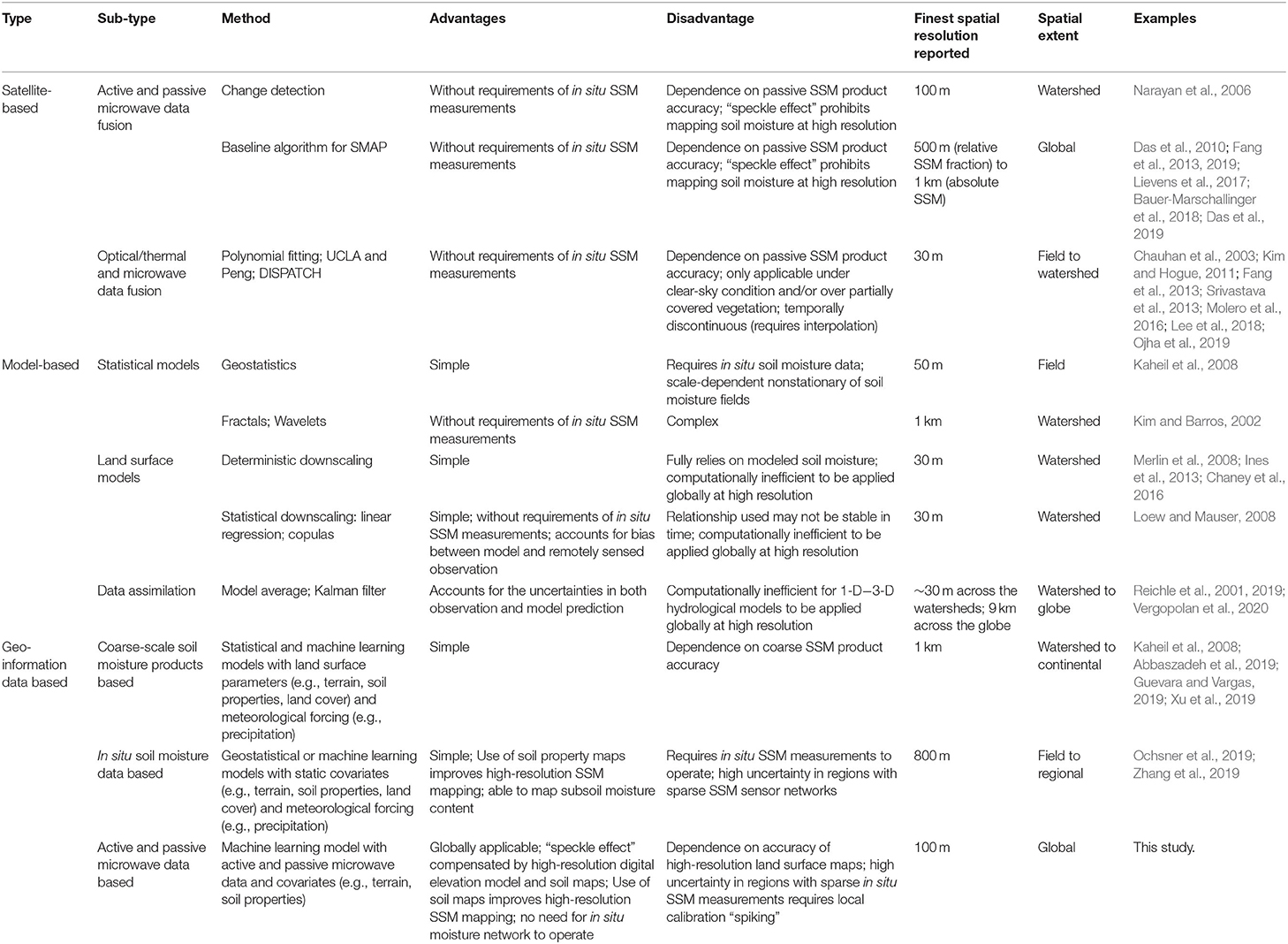
Table 1. A brief summary of spatial downscaling methods for surface soil moisture—SSM (modified from Peng et al., 2017).

In this study, we explore a new global SSM downscaling method that uses machine learning (quantile random forest) to fuse in situ soil moisture network data across the globe, remote sensing data from SMAP, and Sentinel-1, and high-resolution land surface parameters (i.e., terrain parameters, soil properties). Compared with other methods, this geo-information data based approach relies on active and passive microwave data to operate (similar to the change detection method) but it also uses high-resolution land surface parameters (terrain parameters and soil maps) and in situ SSM measurements to improve the model performance by compensating the “speckle effect” of active microwave data.

Our working hypotheses are: (1) a combination of active and passive microwave remote sensing and high-resolution land surface parameters can improve the delineation of SSM at the regional scale (100 m) compared to that established using any one individual dataset with high-resolution land surface parameters compensating the “speckle effect” of backscatter data, and (2) the global model can be used to delineate SSM variations at the field scale (i.e., 10–100 m) with the addition of a small number of field-scale in situ SSM measurements.

Our research questions are: (1) How well can an empirical machine learning model map regional field-scale (100-m) SSM at a 6–12 day interval? (2) How does model performance vary by different continental/regional monitoring systems and land cover types across the globe? (3) How well will a global empirical model established using continental/regional datasets perform at the field scale with and without in situ field-scale soil moisture network measurements? (4) How will the spatial resolution of Sentinel-1 data and the spatial-resolution and accuracy of input soil property maps affect the predicted SSM at the field scale?

Materials and Methods

Remote Sensing and Land Surface Data

Ground in situ SSM measurements from various soil moisture networks were used as training and validation data for the remote sensing and land surface data that were used as covariates to retrieve SSM across the globe. Both remote sensing and land surface datasets were spatially explicit with the remote sensing data time-varying and the land surface datasets time-constant (Figure 2 and Table 2).

TABLE 2

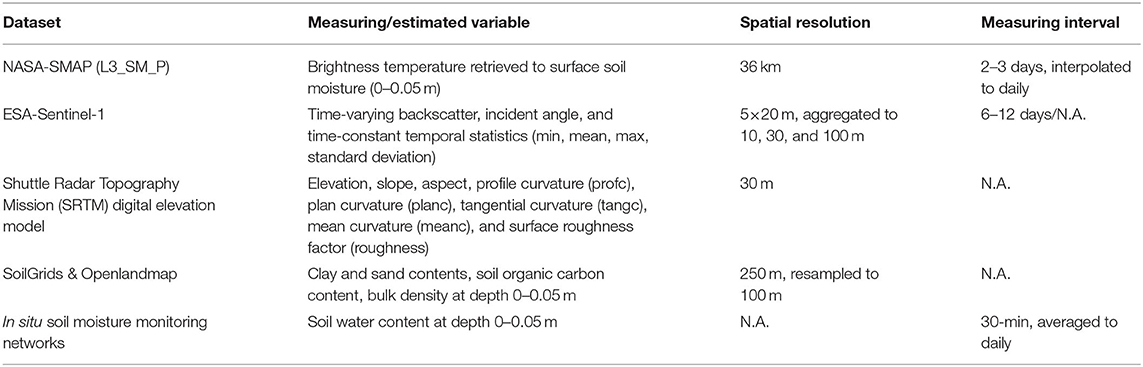
Table 2. Remote sensing and land surface datasets used for modeling surface soil moisture (SSM).

NASA SMAP Mission

The SMAP mission was launched by the NASA, which provides land surface measurements across the globe with a revisit time of 2–3 days. It relies on the simultaneous measurements of L-band backscatter from an active synthetic-aperture radar (SAR) and brightness temperature from a passive L-band radiometer to retrieve SSM (Lievens et al., 2017). The sensors operate at a constant incidence angle. The use of L-band microwave signals enables detection of land surface moisture under moderate vegetation cover, through cloud cover, and during day and night. Since the failure of the radar in 2015, the SMAP mission can only retrieve SSM based on the passive radiometer. In this study, the SMAP_L3_SM_P product was used, which retrieves SSM at 0–0.05 m with a resampled spatial resolution of 36 km × 36 km and a revisit time of 2-3 days across the globe based on a physical model using brightness temperature and ancillary datasets (O'Neill et al., 2015).

SMAP data were downloaded from Earth Data (https://earthdata.nasa.gov/) using the R platform (Version 3.6.0) with the package “smapr” (Version 0.2.1) from March 1st to October 1st between 2016 and 2019. The period was selected to avoid frozen soils within the various soil moisture networks because of the poor performance of SSM retrieval over frozen ground. Afterward, the data were gap-filled pixel-wise using a simple temporal moving average with a window size of 3 days using the “imputeTS” package. The small window size was selected to avoid the smoothing of SSM due to its strong variability over time. This generated SSM estimates at a 36 km × 36 km resolution on a daily basis during the study period, which were used as time-varying covariates for modeling SSM.

ESA Sentinel-1 Mission

Sentinel-1 mission was launched by the European Space Agency (ESA), which consists of C-band SARs situated at a two-satellite constellation operating at dual polarizations: single co-polarization with vertical transmit/vertical receive (abbreviated as VV) and dual-band cross-polarization with vertical transmit/horizontal receive (abbreviated as VH). It measures the land surface backscatter intensity at VV and VH polarizations with a varying incidence angle with a spatial resolution of 5 m × 20 m and a revisit time of 6–12 days. The use of a C-band microwave signal leads to a reduced penetration depth of Sentinel-1's sensors under moderate vegetation cover compared to SMAP. The relationship between SAR backscatter and the dielectric constant of the soil (a function of soil moisture) enables retrieval of SSM from the Sentinel-1 data (Paloscia et al., 2013; Fang et al., 2019). Because the existing global empirical model of the Sentinel-1 mission only retrieves relative SSM instead of absolute soil volumetric water content (Bauer-Marschallinger et al., 2018), and because the physical retrieval model is currently under development (Lievens et al., 2017), the backscatter and incidence angle data were selected as covariates. Here, classical physical models (e.g., Oh et al., 1992; Fung, 1994; Dubois et al., 1995) were not used to retrieve SSM from the Sentinel-1 data because researchers have reported poor performance of the physical models when SSM is large and land surface roughness is high (Merzouki et al., 2011; Lievens et al., 2017).

The backscatter data were preprocessed using the Sentinel-1 Toolbox (https://sentinel.esa.int/web/sentinel/toolboxes/sentinel-1) within the Google Earth Engine platform (https://developers.google.com/earth-engine/sentinel1), which involves thermal noise removal, radiometric calibration, and terrain correction using Shuttle Radar Topography Mission (SRTM) 30-m digital elevation model (Rabus et al., 2003). To minimize the speckle effects of the resampled Sentinel-1 radar data (Gao et al., 2017), additional preprocessing procedures were applied using the Google Earth Engine platform (Gorelick et al., 2017). This was suggested by Bauer-Marschallinger et al. (2018) and involved dynamic masking the extreme backscatter values outside the normal ranges for VV (−5 to −25 dB) and VH (−10 to −30 dB), spatial aggregating to 100 m × 100 m, and filtering with a 3 × 3 Gaussian filter. The processed Sentinel-1 data included backscatter data and incidence angle values at a 100 m × 100 m resolution with a revisit time of 6–12 days, which were used as time-varying covariates for modeling SSM.

To facilitate the retrieving of SSM from Sentinel-1 data, several temporal indices were calculated from the processed Sentinel-1 backscatter images pixel-wise to account for the land surface characteristics, such as temporal minimum, mean, maximum, and standard deviation (SD) of the backscatter data. These temporal statistics of the sensor measurements over time contain characteristics of the soil and vegetation in the field (Huang et al., 2019) and were used as time-constant covariates for modeling SSM.

Terrain Parameters

In addition to remote sensing datasets that can be directed used to retrieve SSM, terrain parameters that characterize topography have been used to indirectly model or downscale SSM (Entekhabi et al., 2010; Malone et al., 2012; Guevara and Vargas, 2019). In this study, a 30-m Shuttle Radar Topography Mission (SRTM) Digital Elevation Model (DEM) was used to calculate several primary and secondary terrain parameters, including slope, aspect, profile curvature (profc), plan curvature (planc), tangential curvature (tangc), mean curvature (meanc), and surface roughness factor (roughness) following (Olaya, 2009; Csillik and Drăguţ, 2018).

Soil Properties

Soil physical and chemical properties affect soil water retention and redistribution in space and time (Mohanty and Skaggs, 2001). Although finer-resolution maps of soil properties are available in many countries where the soil moisture networks are installed (e.g., Grundy et al., 2015; Ramcharan et al., 2018; Chaney et al., 2019), a global map of soil properties was used for here given its consistency across the world. In this study, 250-m resolution maps of soil properties were used, which include clay and sand content, bulk density (BD), soil organic carbon content from the SoilGrids (Hengl et al., 2017). To avoid artifacts in final SSM maps caused by the 250-m input soil property maps, these soil maps were resampled to 100-m using bilinear interpolation using Google Earth Engine.

Land Cover

Land surface characteristics vary with different LC types and had different impacts on the spatial and temporal variations of SSM and the performance of SSM models (Entekhabi et al., 2010). To facilitate the interpretation of the SSM models, a 100-m global land cover (LC) data were downloaded during 2016 from the Copernicus Global Land Service (epoch 2015). Five merged LC types were selected, including cultivated, herbaceous, forest, shrub, and bare land. The LC type was not used as covariates for retrieving SSM because it was not selected as the important variable by the empirical quantile random forest model (results not shown here).

In situ Soil Moisture Monitoring Networks

In situ soil moisture networks have been established across the world to provide long-term climate reference measurements for meteorological monitoring, hydrological modeling, and validating of remote sensing products (Dorigo et al., 2011; Quiring et al., 2016; Bogena et al., 2018). Here, three types of soil moisture networks were used in this study: continental-, regional-, and field- scale networks (Figure 1). A summary of the number of stations used in this study is provided in Table 3. Details about the site characterization of these networks can be found in the references mentioned above.

FIGURE 1

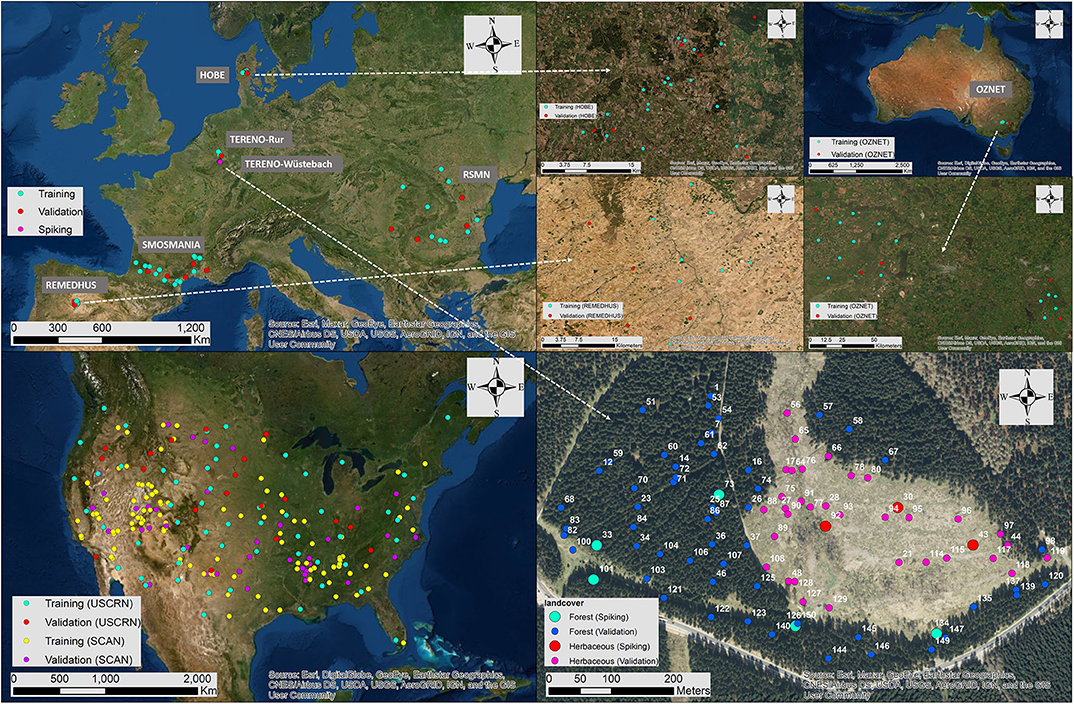
Figure 1. Locations of continental—(SCAN, USCRN), regional—(HOBE, OZNET, REMEDHUS, RSMN, SMOSMANIA, TERENO-Rur), and field—(TERENO-Wüstebach) scale soil moisture networks. Training and validation stations from the continental- and regional- scale networks were highlighted in different colors and the local training (“spiking”) and validation stations from the field-scale network were marked in large and small solid circles, respectively.

TABLE 3

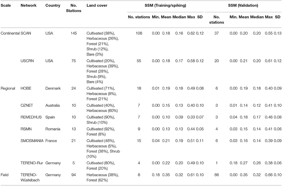
Table 3. Summary statistics of land cover types and surface soil moisture (SSM) at continental—(SCAN, USCRN), regional—HOBE, OZNET, REMEDHUS, RSMN, SMOSMANIA, TERENO-Rur), and field—(TERENO-Wüstebach) scale soil moisture monitoring networks for training/spiking and validation datasets.

Continental-scale soil moisture networks consist of National Oceanic and Atmospheric Administration sponsored US Climate Reference Network (USCRN, Bell et al., 2013) and the United States Department of Agriculture Natural Resources Conservation Service soil climate analysis network (SCAN, Schaefer et al., 2007). These networks are sparsely situated across the USA with several stations within each state, but they cover a variety of climate regimes, terrain parameters, land cover types, and soil texture classes. It was expected that the use of these widely spread networks can provide information on the relationship between climate regimes, terrain parameters, land cover types, and soil texture classes with SSM and improve the robustness and transferability of the SSM model.

Regional-scale soil moisture networks consist of the Danish hydrological observatory (HOBE) in Denmark (Jensen and Illangasekare, 2011), Murrumbidgee soil moisture monitoring networks of the OZNET in New South Wales, Australia (Smith et al., 2012), Soil Moisture Measurement Stations Network of the University of Salamanca, Spain (REMEDHUS) (Martínez-Fernández and Ceballos, 2005), Romania Soil Moisture Network (RSMN) (Haggard et al., 2010), SMOSMANIA network in France (Calvet et al., 2007), and a subset of the TERrestrial ENvironmental Observatories in Germany (TERENO-Rur) (Bogena et al., 2018). These networks were selected because they were located at the regional scale (<50,000 km²) and can be used to characterize variations of surface soil moisture within catchments, and span a variety of soil moisture and climatic regimes each with significant spatial variability. It was expected that soil moisture measurements from these regional-scale networks can provide detailed information for retrieving SSM within the coarse pixels of the SMAP SSM product (36 km). Although there are other in situ soil moisture networks across the globe, we did not use them because either there are too few stations (<4) within the network/too few measurements available during 2016–2019, or the soil moisture sensors had a large measuring footprint (>100 m) such as the cosmic-ray neutron probes.

Establishing Empirical SSM Retrieval Models

Unlike previous studies that downscaled coarse-resolution SSM products (e.g., SMAP, SMOS) using change detection algorithms with fine-resolutions remote sensing data (e.g., Fang et al., 2019; Ojha et al., 2019) or a high-resolution digital elevation model (Guevara and Vargas, 2019), we applied an empirical modeling approach to retrieve SSM from in situ soil moisture network measurements. Although this approach required a large number of training datasets, it may help account for bias within the input covariates (e.g., SMAP SSM) during the modeling process.

Here, a quantile random forest algorithm was used to establish the empirical model. Random Forest is a nonparametric model based on similarities among observations to fit decision trees (Breiman, 2001). To determine a split at a node in a tree, a random subsample of predictor variables is taken to select the predictor that minimizes the regression error. Nodes continue to be split until no further improvement in error is achieved. The prediction is achieved with an adaptive neighborhood classification and regression. Omitted observations, termed the “out-of-bag” sample, are used to compute the regression errors for trees (Breiman, 2001; Hastie et al., 2009). To estimate the quantiles of the predictions, the Quantile Random Forest (QRF) algorithm was applied using the R “quantregForest” package (Version 1.3-7, Meinshausen and Meinshausen, 2017), which estimates the conditional distribution based on a weighted distribution of observed model response values (Meinshausen, 2006). The “train” function from the “caret” function was used to estimate the model parameters based on 5-fold cross-validation with “root mean squared error” as the selection metrics. To avoid overfitting, we compared the models established using 10, 20, 50, and 100 trees with the minimum size of the terminal nodes of 5 and 10. Based on the root mean square error and R² on the training and validation data, the maximum number of trees and minimum size of the terminal nodes were empirically set to 50 and 10, respectively, so that a further increase of the number of “trees” did not significantly improve the model performance for the training dataset and the difference between the root mean square errors of the training and validation dataset was small.

To train the QRF model and evaluate the model performance at the regional scale, two types of validation methods were used. First, the evaluation was done for different LC types with randomly selected 75% stations from all soil moisture networks as the training dataset and the remaining 25% stations from all soil moisture networks as the validation dataset (as shown in Figure 1). Secondly, the evaluation was performed on individual soil moisture networks. To achieve this, the model was trained using coupled SSM measurements and covariates from the continental networks (USCRN and SCAN) and then applied onto the regional networks (HOBE, OZNET, REMEDHUS, RSMN, SMOSMANIA, TERENO-Rur) for validation.

For both evaluation methods, the coefficient of determination (R²), Pearsons' correlation coefficient (r), mean error (ME, bias), and root mean squared error (RMSE, accuracy) were calculated for both calibration (5-fold cross-validation results) and validation datasets using the measured SSM at the stations and predicted SSM from the QRF models.

The SMAP SSM estimates on the training and validation SSM network stations were also used for evaluating the performance of the QRF model. For brevity, we called it the “SMAP model.” It should be noted that we did not validate the performance of SMAP data at the regional scale using individual continental/regional soil moisture sensor networks because there was only one station with the 36-km pixel of SMAP data. Instead, the use of SMAP data was to provide a reference point for assessing the variations of SSM at the regional scale. This is reasonable given that similar benchmarking analyses have been carried in other studies to assess the performance of SMAP and other SSM products when dense soil moisture networks are not available (Lievens et al., 2017; Bauer-Marschallinger et al., 2018; Das et al., 2019; Guevara and Vargas, 2019; Reichle et al., 2019).

Evaluating the Effects of Different Covariates

To evaluate the effects of different input covariates, two methods were used. First, variable importance of the QRF model was calculated based on the mean increase in node purity (IncNodePurity), representing the decrease in the sum of squares by including each covariate. A large IncNodePurity indicates the covariate is more important in the model than others. Second, different types of covariates were dropped in turn (e.g., SMAP, Sentinel-1, terrain parameters, soil properties) to fit the QRF models. The performance of these reduced QRF models was compared against the full model to understand the relative importance of each covariate.

Evaluating the Global SSM Model at the Field Scale With and Without “Spiking” Samples From a Dense Soil Moisture Network

SSM was predicted using the global model onto one field-scale soil moisture network (TERENO-Wüstebach, Germany). The global model used was established with 75% training soil moisture stations across different networks (countries) to account for the hetereogeneity in land surface (Figure 2). The field-scale network consists of ~150 soil sensor stations across a hillslope with elevation increasing from 595 m in the north to 628 m in the south (Bogena et al., 2018). Soil moisture is measured with EC5 and 5TE sensors (Decagon, Devices Inc., Pullman, WA, USA). The mean annual precipitation is about 1,100–1,200 mm and the main vegetation is Norway Spruce (Stockinger et al., 2014). During the late summer of 2013, Spruce trees were clear-cut in an area of 9 ha to initiate the regeneration of near-natural beech forest (Figure 1, Wiekenkamp et al., 2020). In this study, daily averaged SSM data were used from 94 stations from 2016 to 2018. These SSM stations were split into a local training dataset consisting of ~10% randomly selected stations from the total stations (5 under forest and 3 under herbaceous soils) and an independent validation dataset with the remaining stations.

FIGURE 2

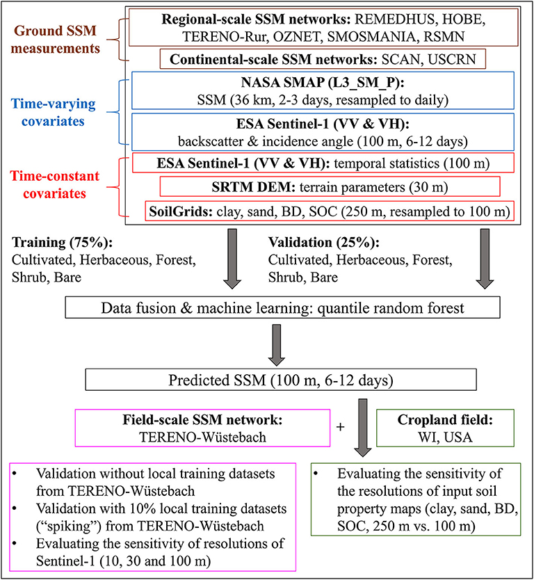
Figure 2. Flowchart of the global surface soil water model established using data fusion and machine learning and different evaluation approaches.

First, we evaluated the performance of the global SSM on the validation dataset without using any local training data. Secondly, we incorporated the 10% local training dataset into the continental and regional dataset and refitted the QRF models before evaluation on the remaining validation dataset. The use of local training dataset for calibrating empirical models (sometimes termed as “spiking”) has been adopted in many other fields such as the soil spectroscopy libraries established using datasets collected from different countries or instruments (Guerrero et al., 2010; Wetterlind and Stenberg, 2010; Viscarra Rossel et al., 2016). This is particularly useful when the empirical models have low transferability where the feature spaces (e.g., land surface parameters) of training and validation datasets vary greatly.

Last, we also evaluated the effects of the resolution of Sentinel-1 data on the model performance and predicted SSM at the field scale. To achieve this, we calculated Sentinel-1 data and their temporal statistics at 10, 30, and 100 m resolutions and used them to refit the QRF models with and without in situ soil sensor measurements. The model performance and the spatial patterns of predicted SSM maps were compared. This analysis was done to assess the sensitivity of Sentinel-1 data on the model performance at the field scale.

Evaluating the Global SSM Model at the Field Scale Using Soil Property Maps With Different Resolutions

The global model established using 75% training soil moisture networks across all the networks was also evaluated ono an 80-ha cropland field in Wisconsin, USA (42.5742° N, 9.1151° W) during the early growing season (cropped with corn) in 2018. Here, the global model was not “spiked” with local soil moisture measurements because field-scale soil moisture networks were not available. Instead, the fitted global model was directly applied to the cropland field. We compared the SSM maps predicted using soil property maps at a 250-m resolution (obtained from Hengl et al., 2017, resampled via bilinear interpolation to 100 m to avoid artifacts) and a 100-m resolution (obtained from Ramcharan et al., 2018). SSM was predicted across the entire field on wet (2018/06/16) and dry (2018/06/28) soil conditions for comparison. The resolution of Sentinel-1 data was held as 100 m (Figure 2). This analysis was done to evaluate the effects of the resolution and accuracy of soil property maps on mapping SSM at the field scale.

Results

Model Performance of the QRF and SMAP Product and Variable Importance

The model performance of the fitted QRF model is presented in Figure 3. The model has an ME of −0.00 m³ m⁻³, RMSE of 0.05 m³ m⁻³, and R² of 0.784 for the training dataset based on 5-fold cross-validation and reduced performance with an ME of 0.00 m³ m⁻³, RMSE of 0.07 m³ m⁻³, and R² of 0.524 for the validation dataset. This indicates that the model was slightly overfitting. The SSM estimates from SMAP had an overall similar performance (no significant difference) for the same validation dataset with an ME of −0.01 m³ m⁻³, RMSE of 0.08 m³ m⁻³, and R² of 0.508. It should be noted that this comparison was only based on the continental to regional soil moisture networks (see sections Delineating SSM Variations at the Field-Scale via Data Fusion, The Effect of “Spiking” on the Global SSM Model, The Effect of Resolutions of Soil Property Maps on the SSM Model for comparison at the field scale).

FIGURE 3

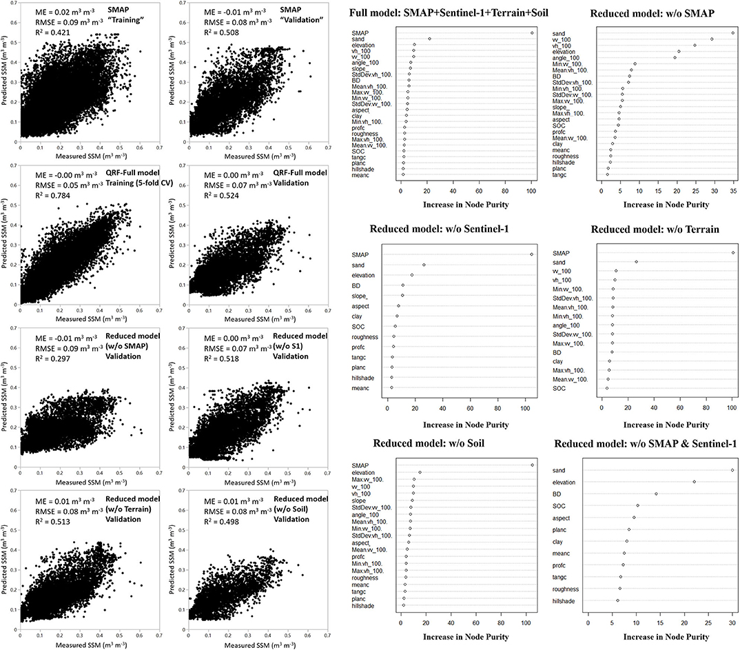
Figure 3. Comparison of the performance and variable importance of quantile random forest (QRF) models on regional- and continental- scale training (70% of the stations from all networks) and validation (remaining 30% stations from all networks) datasets. The models were established using different combinations of input covariates. R2, coefficient of determination; ME, mean error; RMSE, root mean squared error.

The importance of the variables is presented in Figure 3. SMAP was ranked as the most important time-varying variable, followed by Sentinel-1 backscatter data measured at VH and VV polarizations, and incidence angle of the Sentinel-1. In terms of the time-constant variables, sand content was most important, followed by elevation, slope, the temporal SD of VH backscatter data, bulk density, temporal mean of VH backscatter data, and other variables.

The importance of different variables was also demonstrated after dropping each of the covariates from the full model. As shown in Figure 3, the reduced models had worse performance compared to the full model. Particularly, dropping SMAP data significantly reduced the model performance, followed by soil properties and terrain parameters. It is noted that at the continental to regional scales, the reduced model established without Sentinel-1 data and their temporal statistics only had a slightly worse performance than the full model (Reduced model: ME = 0.00 m³ m⁻³, RMSE = 0.07 m³ m⁻³, R² = 0.518).

Model Performance of the QRF and SMAP Product Within Different Land Cover Types

Pearson's r, ME, and RMSE calculated between measured SSM from the in situ soil moisture networks and predicted SSM from the QRF model or SMAP were used to evaluate the model performance within different land cover types at each of the validation soil moisture stations (see Table 4 for summary statistics of the training and validation datasets). As shown in Figure 4, the empirical QRF full model established via a combination of SMAP, Sentinel-1 (aggregated at 100 m) and land surface parameters have similar performance (non-significant difference) compared to the SMAP SSM estimates at the continental to regional scales.

TABLE 4

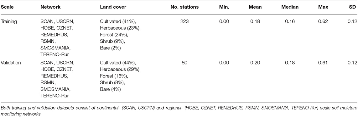
Table 4. Summary statistics of land cover and surface soil moisture (SSM) at the training and validation datasets evaluated by land cover types.

FIGURE 4

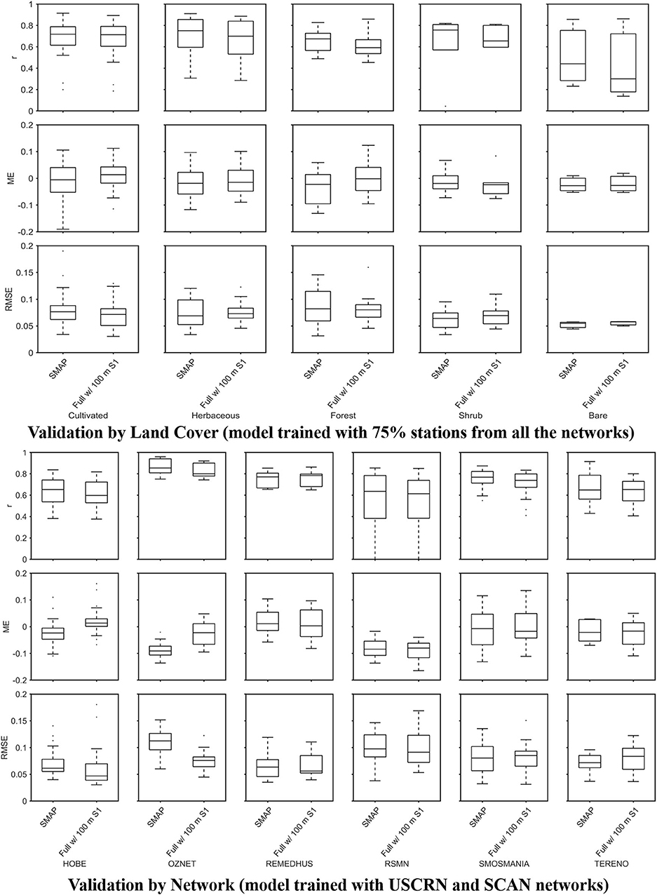
Figure 4. Boxplots of the performance of SMAP L3 product (SMAP) and quantile random forest (QRF) models on individual regional- and continental- scale validation station evaluated by land cover (trained and validated using 70 and 30% of stations from all networks) and by network (trained using continental networks—USCRN and SCAN and validated using other regional networks). The QRF models were established using all input covariates with Sentinel-1 data aggregated at 100 m (Full w/100 m S1). R2, coefficient of determination; ME, mean error; RMSE, root mean squared error.

However, the performance of both SSM models varied greatly across the LC types. It was evident that the full QRF and SMAP models were more accurate under herbaceous (mean r = 0.682 vs. 0.696, RMSE = 0.08 vs. 0.07 m³ m⁻³) and cultivated (mean r = 0.624 vs. 0.621, RMSE = 0.07 vs. 0.08 m³ m⁻³), than shrub (mean r = 0.583 vs. 0.626, RMSE = 0.07 vs. 0.06 m³ m⁻³), forest (mean r = 0.611 vs. 0.654, RMSE = 0.08 vs. 0.09 m³ m⁻³), and bare soils (mean r = 0.433 vs. 0.510, RMSE = 0.06 vs. 0.05 m³ m⁻³).

It should also be noted that large variations of model performance (i.e., Pearson's r, ME, RMSE) were observed for all land cover types among different ground SSM stations, indicating strong heterogeneity of land surface parameters at the field scale that cannot be captured by the resolution of the input remote sensing or land surface parameters. In summary, we note that both the full QRF model and SMAP were able to retrieve SSM dynamics under herbaceous, cultivated, shrub, and forest soils at the continental to regional scales with a moderate level of uncertainty (a global performance of ME of 0.00 m³ m⁻³, RMSE of 0.07 m³ m⁻³, and R² of 0.524 for the QRF model and ME of −0.01 m³ m⁻³, RMSE of 0.08 m³ m⁻³, and R² of 0.508 for the SMAP model).

Model Performance of the QRF and SMAP Product Within Different Networks

The model performance was also evaluated for different soil moisture networks with the continental-scale USCRN and SCAN networks as the training datasets and the remaining regional-scale networks as the validation dataset. As shown in Figure 4, the model performance varies with the network. Both the full QRF and SMAP models performed well in REMEDHUS (mean r = 0.754 vs. 0.747, RMSE = 0.07 vs. 0.07 m³ m⁻³), followed by SMOSMANIA (mean r = 0.707 vs. 0.754, RMSE = 0.08 vs. 0.08 m³ m⁻³), HOBE (mean r = 0.616 vs. 0.645, RMSE = 0.06 vs. 0.07 m³ m⁻³), TERENO (mean r = 0.632 vs. 0.669, RMSE = 0.08 vs. 0.07 m³ m⁻³), and moderately well in RSMN (mean r = 0.538 vs. 0.538, RMSE = 0.10 vs. 0.10 m³ m⁻³). Interestingly, the QRF model outperformed SMAP model in OZNET (mean r = 0.827 vs. 0.859, RMSE = 0.08 vs. 0.11 m³ m⁻³). These results indicated that the empirical QRF model has a relatively good transferability across the different networks and can be used to estimate SSM at the regional scales outside the USA. However, the performance of the models would vary in different regions, most likely due to the variability of land surface parameters such as LC types (Table 3).

Delineating SSM Variations at the Field-Scale via Data Fusion

Although the performance of the coarse-resolution SMAP model was similar to that of the QRF model at the regional to continental scales, the SMAP maps cannot reveal spatial SSM variations at the field scale. As shown in Figure 5, dropping any covariate from the full model (e.g., SMAP, Sentinel-1, terrain parameters, soil properties) would reduce the model performance evaluated at the field-scale soil moisture networks. The SMAP model was able to pick up the temporal variations of SSM across the field from 2016 to 2018 (Figure 6) and at relatively wet (2018/04/05) and dry (2018/04/23) soil moisture conditions (Figure 7) but it failed to delineate within-field variations in SSM across the TERENO-Wüstebach site. By comparison, the data fusion based full QRF model delineated both temporal dynamics in SSM and spatial variations across the field between forest and herbaceous soils and along the slope gradient (Figures 6, 7).

FIGURE 5

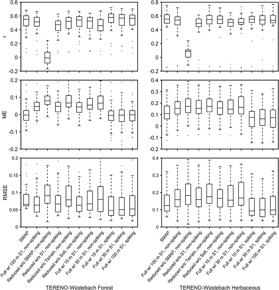
Figure 5. Boxplots of the performance of SMAP L3 product (SMAP) and quantile random forest (QRF) models on individual field-scale validation station (TERENO-Wüstebach) evaluated by land cover (forest vs. herbaceous). The QRF models were first established without local training datasets using different input covariates including full model with Sentinel-1 aggregated at 100 m (Full w/100 m S1, non-spiking) and the corresponding reduced models by dropping SMAP (Reduced w/o SMAP, non-spiking), Sentinel-1 (Reduced w/o S1, non-spiking), terrain parameters (Reduced w/o Terrain, non-spiking), or soil properties (Reduced w/o Soil), and full models with Sentinel-1 aggregated at 10 m (Full w/10 m S1, non-spiking) and 30 m (Full w/10 m S1, non-spiking). QRF models were also established by including 10% local training stations at TERENO-Wüstebach (5 forest stations and 3 herbaceous stations, see Figure 1) with different resolutions of Sentinel-1 data (e.g., Full w/10 m S1, spiking). R2, coefficient of determination; ME, mean error; RMSE, root mean squared error.

FIGURE 6

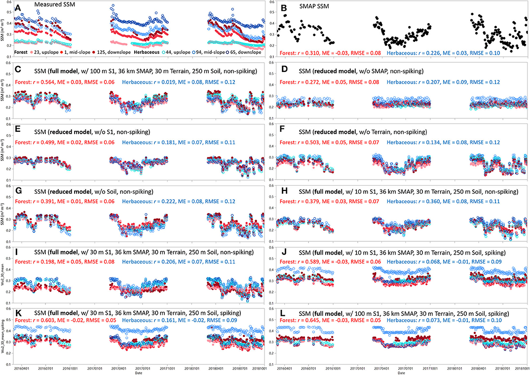
Figure 6. Measured (A) vs. predicted surface soil moisture (SSM, m³ m⁻³) from SMAP L3 product (SMAP, B) and the quantile random forest (QRF) models at selected stations of the field-scale soil moisture network (TERENO-Wüstebach). The QRF models were first established without local training datasets using different input covariates including full model with Sentinel-1 aggregated at 100 m (C) and the corresponding reduced models by dropping SMAP (D), Sentinel-1 (E), terrain parameters (F), or soil properties (G), and full models with Sentinel-1 aggregated at 10 m (H) and 30 m (I). QRF models were also established by including 10% local training stations with different resolutions of Sentinel-1 data at 10 m (J), 30 m (K), and 100 m (L). R2, coefficient of determination; ME, mean error; RMSE, root mean squared error. Validation stations under forest: 23 (upslope), 1 (mid-slope) and 125 (downslope); validation stations under herbaceous: 44 (upslope), 94 (mid-slope), and 65 (downslope).

FIGURE 7

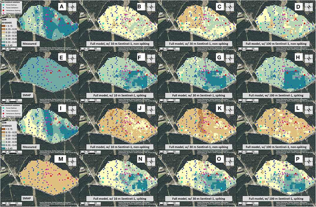
Figure 7. Measured (interpolated soil moisture network measurements using inverse distance weighing, A,I) vs. predicted surface soil moisture (SSM, m³ m⁻³) from the SMAP L3 product (SMAP, E,M) and quantile random forest (QRF) models on wet (2018/04/05, top) and dry (2018/04/23, bottom) soil moisture conditions across the field-scale TERENO-Wüstebach soil moisture network. The QRF models were established using different input covariates without (non-spiking, B–D,J–L) and with (spiking, F–H,N–P) local training datasets and using Sentinel-1 aggregated at 10, 30, and 100 m.

The effects of the spatial resolutions of the Sentinel-1 data (and their temporal statistics) were also presented. Although SSM maps generated with Sentinel-1 data aggregated at different resolutions showed differences in SSM at 10, 30, and 100 m resolutions (Figures 6, 7), the overall mean model performance evaluated at the independent field-scale soil moisture stations were not significantly different (Figure 5).

The Effect of “Spiking” on the Global SSM Model

The effect of incorporating local training dataset to the global SSM model (“spiking”) was presented. When the global SSM model was applied to the field without using any local training dataset, it can delineate the variations of SSM over time and across the field under forest and herbaceous soils and along the slope (e.g., Figures 6C, 7B–D,J–L). However, the global SSM models were largely biased with mean ME values of 0.07, 0.08, and 0.06 m³ m⁻³ under forest (0.00 m³ m⁻³ for SMAP) and mean ME values of 0.16, 0.16, and 0.15 m³ m⁻³ under herbaceous soils (0.10 m³ m⁻³ for SMAP) for full models established using 10, 30, and 100 m Sentinel-1, respectively. In addition, the spatial variations (spread) of SSM were smoothed without the use of any “spiking” datasets compared to measured SSM (Supplementary Figures 1–3). This suggested the transferability of the empirical model was poor from the regional scale to field scale without local calibration data.

After 10% of the local training data were added, the bias values of the global SSM models significantly reduced with mean ME values of −0.00, −0.01, and −0.01 m³ m⁻³ under forest (significantly different from non-spiking models with P < 0.001) and mean ME values of 0.07, 0.08, and 0.08 m³ m⁻³ under herbaceous soils (significantly different from non-spiking models with P < 0.05) (Figure 5). As shown in Figures 6J–L, 7F−H,N–P and Supplementary Figures 1–3, the predicted SSM from these “spiked” QRF models showed similar spatial patterns of SSM as measured by the in situ soil moisture sensors while SMAP SSM was uniform across the field on individual days. In addition, the spread of QRF models estimated SSM (as shown in histograms in Supplementary Figures 1–3) were also greatly improved after the “spiking” as compared to non-spiking models and the SMAP SSM. This suggests the transferability of the empirical model can be improved by including a small number of local training datasets into the model.

Here, we did not estimate the spatial structure of the measured SSM vs. predicted SSM across the field due to the small number of SSM stations used to generate the maps of measured SSM. This is because previous studies have suggested a minimum number of 100 sample points is required to accurately estimate the variogram parameters (Webster and Oliver, 1992). Instead, we plotted the measured SSM interpolated via inverse distance weighing using in situ soil moisture sensors vs. predicted SSM by the QRF model with 10-m Sentinel-1 and with the “spiking” dataset. As shown in Figure 8, from 2018/04/05 to 2018/04/23, both measured SSM and predicted SSM displayed a drying pattern across the field. The “spiked” QRF model was accurate for most parts of the field with an error of less than 0.05 m³ m⁻³, where “spiking” stations were located (Figure 8). However, the QRF model underestimated SSM in herbaceous soils in the center of the field and overestimated SSM in forest soils mostly in the western and eastern central regions of the field. The former may be caused by the distribution of sensors in the center of the field (e.g., a local valley), which led to small variations of SSM observed in the central region. The latter may be because no “spiking” samples were selected from these regions (Figure 8). To improve the performance of the empirical model in these regions, more training datasets are required to capture the feature spaces that have different soil moisture patterns due to different LC types, topography, soil properties, and climate patterns compared to the patterns observed in the existing regional and continental scale datasets.

FIGURE 8

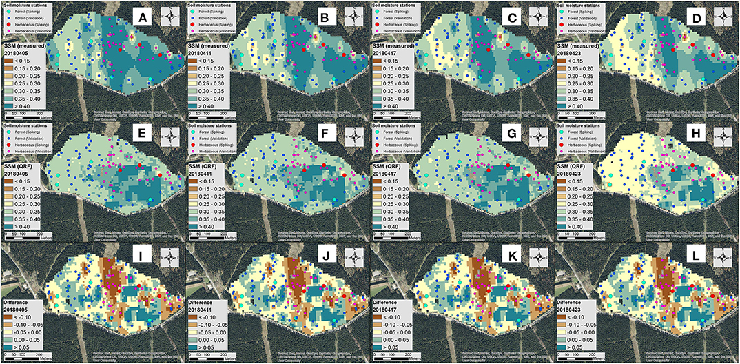
Figure 8. Measured (interpolated soil moisture network measurements using inverse distance weighing, A–D) vs. predicted surface soil moisture (SSM, m³ m⁻³) from the quantile random forest (QRF) model during a drying event from 2018/04/05 to 2018/04/23 across the field-scale TERENO-Wüstebach soil moisture network (E–H). The QRF model was established with local training datasets (spiking) and Sentinel-1 aggregated at 10 m. The differences were calculated by subtracting QRD model estimates pixel-wise with measured SSM values (I–L).

The Effect of Resolutions of Soil Property Maps on the SSM Model

The effects of the resolution and accuracy of soil property maps on predicting SSM at the field scale are presented in Figure 9. It was noted that the resampled 250-m sand content map (Figure 9A) presented a similar trend to the 100-m map (Figure 9B) but large differences were observed in the northwest and southeast corners of the field (larger than 9%, Figure 9C). Similar results were also identified for other properties and not shown here.

FIGURE 9

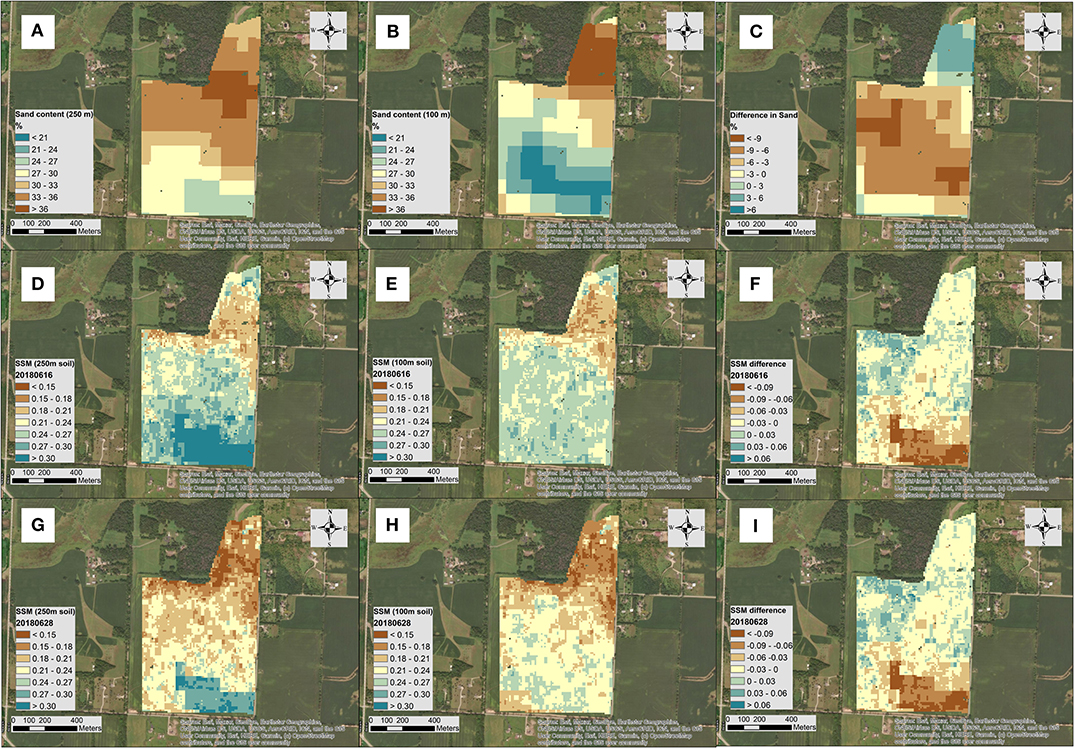
Figure 9. Maps of soil sand content (%) at 250 m (obtained from Hengl et al., 2017, resampled to 100 m with bilinear interpolation, A) and 100 m (obtained from Ramcharan et al., 2018, B) with the predicted surface soil moisture (SSM, m³ m⁻³) from the quantile random forest (QRF) model (without local calibration— “spiking”) using the 250 m (D,G) and 100 m (E,H) soil property maps on wet (2018/06/16) and dry (2018/06/28) soil conditions across a cropland in Wisconsin, USA. The differences in soil sand content (C) and differences in estimated SSM between 100 and 250 m soil property maps (F,I) are also presented.

SSM predicted from 250- and 100-m soil property maps (clay, sand, BD, and SOC) showed similar spatial patterns across the field. Under wet conditions, predicted SSM varied from 0.15 to larger than 0.30 m³ m⁻³ with the use of the 250-m soil maps (Figure 9D) and from 0.15 to 0.30 m³ m⁻³ with the 100-m soil maps (Figure 9E). Under dry conditions, predicted SSM varied from less than 0.15–0.30 m³ m⁻³ with the 250-m soil maps (Figure 9G) and less than 0.15–0.27 m³ m⁻³ with the 100-m soil maps (Figure 9E). For most parts of the field, the differences of SSM maps due to the use of different resolutions of soil maps were small (absolute difference <0.03 m³ m⁻³). However, compared to the maps established using 100-m soil data, use of 250-m soil property maps led to a slight under-estimation of SSM in the northwest corner (~0.06 m³ m⁻³) but a large over-estimation of SSM in the southeast corner (~0.09 m³ m⁻³). The regions of largest differences were consistent with the differences in input sand content maps.

Discussion

Model Performance in Different Land Cover and Networks

In terms of the model performance between different LC types, the empirical QRF model is similar to the 36-km SMAP_L3 SSM product under cultivated, herbaceous and bare soils. This indicates that the data fusion based model can retrieve SSM temporal dynamics well when the SMAP model performs well. A slightly better performance was observed in SMAP data under forest and shrub (Figure 4), which is most likely due to the use of a C-band microwave signal from Sentinel-1 that has a reduced penetration depth compared to the L-band SMAP passive microwave radiometer under moderate to dense vegetation cover conditions (Lievens et al., 2017). In terms of the overall mean r values for both SMAP and QRF models (0.433 vs. 0.510, Figure 4), this may be caused by the small number of training soil moisture stations (7 from USCRN and SCAN) and the overall dry land surface conditions at these sites.

The independent network-based validation results shown in Figure 4 suggest that the empirical SSM model can predict SSM outside the training stations across the globe. However, it should also be noted that the performance of the empirical model varies with locations. It can be concluded that the empirical SSM model performs well in OZNET, REMEDHUS, SMOSMANIA, HOBE, TERENO, and under similar land surface conditions to these networks. In terms of the moderate performance of the empirical model and the SMAP model in RSMN, this may be attributed to the complex land surface characteristics (terrain and soil types) within the mountainous regions of the Romania Soil Moisture Network (Haggard et al., 2010) that affect the relationships between SSM with backscatter and brightness temperature collected from Sentinel-1 and SMAP satellites.

Particularly, it should be noted that the empirical model outperforms the SMAP model in OZNET, which is consistent with the distribution of cultivated and herbaceous land in this region (no shrub or forest) (Table 3). This indicates that the empirical model approach can be potentially applied to agricultural regions for irrigation management where information about the field-scale variations of soil moisture is needed but cannot be obtained from coarse-resolution remote sensing platforms like SMAP. This needs to be further tested in the future with intensive ground soil moisture surveys or dense soil moisture networks installed during the crop growing seasons (Huang et al., 2019; Ojha et al., 2019).

A Tradeoff Between Spatial and Temporal Resolutions of Remote Sensing Soil Moisture Products

Current remote sensing soil moisture missions operating at the global scale are based on passive microwave (e.g., SMOS, SMAP, SMAR2, ASCAT), active microwave (e.g., Sentinel-1, RADARSAT-2) and gravity (GRACE). As shown in Figure 10 and summarized by others (Robinson et al., 2008; Wang and Qu, 2009; Ochsner et al., 2013; Vereecken et al., 2014), there is a tradeoff between the spatial and temporal resolutions of these satellites. In general, active microwave satellites have a fine spatial resolution less than 1 km but the temporal resolution (revisit time) is more than one week. By contrast, passive microwave satellites have a coarse spatial resolution larger than 10 km but the temporal resolution is higher (1–3 days). The gravity-based mission (GRACE) measures soil water in the deep profile and has a large spatial resolution (>100 km) with a temporal resolution of ~1 month (Scanlon et al., 2019).

FIGURE 10

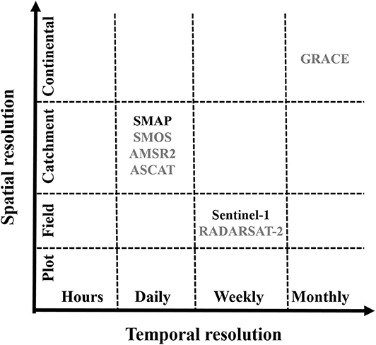
Figure 10. Spatial and temporal resolutions of current remote sensing soil moisture monitoring satellites. Satellites used in this study are highlighted in black and other satellites designed to monitor soil moisture are marked in gray.

The empirical SSM model established here has a spatial resolution of ~100 m and revisit time of 6–12 days (depending on the location of the study sites) across the globe. Many researchers have attempted to retrieve SSM at a similar (100 m) or higher (30 m) spatial resolution using Sentinel-1 data at the field scale using a larger number of ground-based SSM measurements (e.g., Alexakis et al., 2017; Gao et al., 2017; Attarzadeh et al., 2018). However, the model performance may deteriorate with increasing spatial resolution. Based on the work of Bauer-Marschallinger et al. (2018), the radar signal has a large noise (speckle effect) at the field scale due to the interference with heterogeneous vegetation, terrain surface, and soil properties. These authors suggested upscaling Sentinel-1 data to a larger spatial resolution (e.g., 500 m) to reduce the sensor's noise. Similarly, Ojha et al. (2019) explored the potential to use a stepwise disaggregation method with the disaggregation based on physical and theoretical scale change (DISPATCH) algorithm to map SSM using SMAP, MODIS, and Landsat data and found that an intermediate spatial resolution of aggregation is required to maximize the model performance.

In this study, we evaluated the effects of spatial resolutions of Sentinel-1 data on the performance of the global SSM model on the field-scale soil moisture network. It was found that the model performance did not vary significantly with each other when the resolutions of Sentinel-1 data changed from 10 to 30 m and 100 m. This was consistent with the finding of Fang et al. (2019) and was most likely attributed to the intrinsic variability and spatial dependence of SSM at the field scale across the field-scale network. In addition, the use of high-resolution terrain parameters and soil property maps may compensate for the loss of spatial information of land surface parameters (e.g., 30-m DEM) when the resolution of Sentinel-1 data changes.

The limitation of in situ soil moisture sensor networks used in this study should also be noted. In this study, all the soil moisture measurements used provide data at a local scale (<1 m²) while the Sentinel-1 data have an approximate resolution of 10 m. There are two potential solutions for future improvement. One approach is to use in situ soil moisture networks that can collect soil moisture information across a large radius [e.g., cosmic-ray neutron probes, refer to Franz et al., 2015; Montzka et al., 2017, for examples]. In addition, it is possible to generate “soil moisture observation data” that has a similar scale to the remote sensing data for building the SSM models using different upscaling approaches or land surface models (e.g., Crow et al., 2005, 2012; Qin et al., 2013; Wang et al., 2015).

Potential for Field-Scale Research and Applications

The relatively good transferability of the empirical QRF model at the continental to regional scales across different soil moisture networks (from USCRN and SCAN to others) shows its potential to predict SSM in regions where no in situ soil moisture measurements are available. However, care should be taken when applying this model to map SSM at the field scale because the performance can vary with the location. The retrieved SSM maps from the QRF at the field-scale soil moisture network delineate distinct patterns in SSM controlled by land cover and topography, which cannot be obtained from the coarse-resolution SMAP product. Without local calibration, the model may have a large bias compared to the SMAP product but can still delineate the distribution of SSM across the field and over time. When additional information about the study field is available, such as the a small number of local in situ soil moisture sensors, the global QRF model can be improved greatly using the “spiking” method illustrated in this study. Particularly, “spiking” improves the variability in mapped SSM, which better approximates the variability of the measured SSM (Figures 7, 8, and Supplementary Figures 1–3). In this regard, the empirical data fusion-based QRF model established here is an adaptable model and can be improved with the addition of localized SSM measurements from in situ soil moisture networks in the future (Liu et al., 2018). This is equivalent to the development of a global soil visible near-infrared spectroscopy library that can be adapted to field-scale studies with the addition of localized “spiking” dataset (Guerrero et al., 2010; Wetterlind and Stenberg, 2010; Viscarra Rossel et al., 2016).

Many researchers have proposed methods to downscale soil moisture products using empirical or statistical methods (e.g., Fang et al., 2013; Srivastava et al., 2013; Ojha et al., 2019; Xu et al., 2019), process models (e.g., Merlin et al., 2008), data assimilation methods (e.g., Reichle et al., 2019; Vergopolan et al., 2020) and more (Table 1 and Peng et al., 2017). As shown in this study, a combination of Sentinel-1 data and high-resolution land surface parameter maps outperformed the models established using a subset of these ancillary data. This demonstrates the importance of including high-resolution land surface parameters in the SSM models and using them to constrain the estimation of SSM when the accuracy of passive SSM products is low in certain regions across the globe. As demonstrated in previous studies, other high-resolution satellite data (e.g., optical bands from Landsat) have also been used to downscale soil moisture maps (e.g., Lee et al., 2018; Ojha et al., 2019). This indicates the potential to further downscale coarse-scale satellite soil moisture maps across the globe to a finer spatial resolution (e.g., 30–100 m) using a combination of high-resolution land surface parameters (e.g., digital elevation model, soil properties, leaf area index, land cover), high-resolution remote sensing data (e.g., Sentinel-1, Landsat), as well as in situ field-scale soil moisture networks.

Limitations and Future Work

In this study, a random selection of local training soil moisture sensor measurements was used to improve the empirical model at the field scale. Future research is needed to explore the best spatial sampling design for selecting “spiking” stations so that the variations in land surface parameters can be better accounted for in the ML model. It is also possible to assign different weights to the original and spiking datasets due to the limited number of field-scale in situ soil moisture stations across the world. Potential solutions to include applying bootstrapping sampling for the training datasets or other simulation-based approaches.

Our study demonstrates the importance of soil property map for mapping soil moisture variations. Here, the soil property maps were established from machine learning algorithms that may contain large uncertainty in regions where soil core/profile samples were not available, such as central Asia and central Australia (Hengl et al., 2017). The uncertainty of soil property maps may affect the accuracy of soil moisture maps in these regions. Furthermore, Hengl et al. (2017) reported that the R² values for predicted sand, clay, SOC, and BD at the 250-m resolution from SoilGrids were 0.79, 0.73, 0.64, and 0.76, respectively. Given that sand content has a strong contribution in our QRF model (~20% of increase in node purity of the full QRF model), it may cause a decrease of ~4% R² [20% × (1–0.79)] of the full QRF model for estimating SSM (without considering co-variance between other covariates). In our study, at the southeastern corner of the cropland field, soil sand content (Figure 9C) and bulk density (data not shown here) show large uncertainty between the 100-m and 250-m maps, which leads to large uncertainty in SSM maps (Figure 9). This suggests that an accurate soil property map is required when in situ SSM measurements are not available. In addition, previous studies have reported that the use of high-resolution soil maps can improve mapping soil moisture variations at the field scale via mechanistic models (e.g., Chaney et al., 2016; Vergopolan et al., 2020). Therefore, it is worth further investigating the effects and sensitivity of the resolution and uncertainty of soil property maps on mapping soil moisture at the field scale via empirical and mechanistic models. To achieve this, both high-resolution soil property maps and dense soil moisture sensor network measurements need to be collected.

Another disadvantage of the current empirical model is its temporal resolution, which is 6–12 days globally (more frequently in Europe) as controlled by Sentinel-1 data. Future research is required to gap-fill the SSM maps to obtain close to real-time SSM maps. This could be realized using space-time statistical method (Jost et al., 2005), assimilating other remote sensing data such as MODIS land surface temperature (e.g., Gao et al., 2006; Poggio and Gimona, 2017; Ojha et al., 2019) or geostationary satellite hourly surface reflectance (e.g., Yang et al., 2017; Lei et al., 2020), or via mechanistic modeling schemes (e.g., Or and Lehmann, 2019; Vergopolan et al., 2020).

In addition, future research is also required to map soil water content below the surface, particularly within the root zone, as soil water content often varies greatly with depth within the soil profile (Li et al., 2019). To achieve this, empirical and analytical models can be established based on the retrieved SSM maps over a long-term period (Arya et al., 1983; Jackson et al., 1987; Wagner et al., 1999; Gouweleeuw, 2000; Jackson, 2002; Ceballos et al., 2005; Albergel et al., 2008; Sadeghi et al., 2019a,b). Alternatively, ground-based proximal soil sensors can be used to provide estimates of soil texture and hydraulic properties at the field scale at depths (e.g., Robinson et al., 2008; Striegl and Loheide, 2012; Gibson and Franz, 2018). This high-resolution soil information can be included into the established QRF model in this study (similar to the cropland example) to provide estimates of SSM at the field scale and be further combined with mechanistic water balance models via data assimilation to model the movement of soil water within the vadose zone (e.g., Das and Mohanty, 2006; Vereecken et al., 2016; Huang et al., 2017).

Conclusions

An empirical surface soil moisture (SSM) model was established via data fusion of a number of in situ soil moisture networks at the continental and regional scales, active and passive microwave remote sensing data (Sentinel-1 and SMAP) and land surface parameters (e.g., terrain parameters, soil properties) using quantile random forest (QRF) algorithm. The model had a spatial resolution of 100 m and performed moderately well (R² = 0.52, RMSE = 0.07 m³ m⁻³) across the globe under cultivated, herbaceous, forest, and shrub soils. The model has a good transferability at the regional scale across different soil moisture networks. SSM was mapped using the empirical SSM model across a field-scale soil moisture network at the TERENO-Wüstebach site, Germany, and an 80-ha cropland field in Wisconsin, USA.

The QRF model was relatively insensitive to the resolution of Sentinel-1 data due to the use of land surface parameters but was affected by the resolution and accuracy of soil property maps. It is concluded that the empirical model can delineate variations of SSM at the field scale under forest, herbaceous, and cultivated soils under various soil moisture conditions with the bias greatly reduced after including local training datasets via “spiking”.

The SSM model is an adaptable model, which can be further improved by including a small number of in situ soil moisture measurements at the field scale for research and applications. Further research is required to improve the temporal resolution of the SSM model and map soil water content within the root zone.

Data Availability Statement

Publicly available datasets were analyzed in this study. This data can be found here: https://github.com/soilsensingmonitoring.

Author Contributions

JH: data downloading and processing, writing the manuscript, editing the manuscript, and experimental design. AD, JZ, AH, PS, SL, YZ, ZZ, and FA: writing the manuscript, editing the manuscript, and experimental design. HB: data downloading and processing and editing the manuscript. All authors: contributed to the article and approved the submitted version.

Conflict of Interest

The authors declare that the research was conducted in the absence of any commercial or financial relationships that could be construed as a potential conflict of interest.

Acknowledgments

We acknowledge the USDA Hatch project for providing support for the project. We acknowledge HOBE, OZNET, REMEDHUS, RSMN, SMOSMANIA, TERENO, SCAN, USCRN, National Soil Moisture Network, and International Soil Moisture Network for providing the surface soil moisture measurements. We acknowledge SoilGrids & Openlandmap, Ramcharan et al. (2018), NASA, and the US Geological Survey for providing maps of land surface parameters. We also acknowledge ESA and NASA for providing land surface and soil moisture products. We acknowledge the editor Dr. Jianzhi Dong and three reviewers for their constructive comments on improving the manuscript. The final model, training and validation datasets, R codes, along with the local training (spiking) data have been shared on the GitHub for other researchers to use for research and applications at the field scale (https://github.com/soilsensingmonitoring). Due to the heterogeneous nature of land surface parameters across the globe, we recommend the researchers to use the model established using 75% soil moisture stations across all continental/regional/field scale networks.

Supplementary Material

The Supplementary Material for this article can be found online at: https://www.frontiersin.org/articles/10.3389/frwa.2020.578367/full#supplementary-material

References

Abbaszadeh, P., Moradkhani, H., and Zhan, X. (2019). Downscaling SMAP radiometer soil moisture over the CONUS using an ensemble learning method. Water Resour. Res. 55, 324–344. doi: 10.1029/2018WR023354