Integrated Modelling to Support Analysis of COVID-19 Impacts on London's Water System and In-river Water Quality

Dobson, Barnaby; Jovanovic, Tijana; Chen, Yuting; Paschalis, Athanasios; Butler, Adrian; Mijic, Ana

doi:10.3389/frwa.2021.641462

ORIGINAL RESEARCH article

Front. Water, 23 April 2021

Sec. Water and Built Environment

Volume 3 - 2021 | https://doi.org/10.3389/frwa.2021.641462

This article is part of the Research Topic Assessment of the Impact of Covid-19 Pandemic on Water, Environment and Related Ecological and Human Systems View all 3 articles

Integrated Modelling to Support Analysis of COVID-19 Impacts on London's Water System and In-river Water Quality

$\nBarnaby Dobson$ Barnaby Dobson¹^*

Tijana Jovanovic²

Yuting Chen¹

Athanasios Paschalis¹

Adrian Butler¹

Ana Mijic¹

¹Department of Civil and Environmental Engineering, Imperial College London, London, United Kingdom
²British Geological Survey, Nottingham, United Kingdom

Due to the COVID-19 pandemic, citizens of the United Kingdom were required to stay at home for many months in 2020. In the weeks before and months following lockdown, including when it was not being enforced, citizens were advised to stay at home where possible. As a result, in a megacity such as London, where long-distance commuting is common, spatial and temporal changes to patterns of water demand are inevitable. This, in turn, may change where people's waste is treated and ultimately impact the in-river quality of effluent receiving waters. To assess large scale impacts, such as COVID-19, at the city scale, an integrated modelling approach that captures everything between households and rivers is needed. A framework to achieve this is presented in this study and used to explore changes in water use and the associated impacts on wastewater treatment and in-river quality as a result of government and societal responses to COVID-19. Our modelling results revealed significant changes to household water consumption under a range of impact scenarios, however, they only showed significant impacts on pollutant concentrations in household wastewater in central London. Pollutant concentrations in rivers simulated by the model were most sensitive in the tributaries of the River Thames, highlighting the vulnerability of smaller rivers and the important role that they play in diluting pollution. Modelled ammonia and phosphates were found to be the pollutants that rivers were most sensitive to because their main source in urban rivers is domestic wastewater that was significantly altered during the imposed mobility restrictions. A model evaluation showed that we can accurately validate individual model components (i.e., water demand generator) and emphasised need for continuous water quality measurements. Ultimatly, the work provides a basis for further developments of water systems integration approaches to project changes under never-before seen scenarios.

Introduction

Throughout 2020, countries around the world have been taking extensive anti-contagion measures to manage the impact of the COVID-19 pandemic (Hsiang et al., 2020). Many measures have led to reductions in mobility and economic activity with an associated improvement in the natural environment (Arora et al., 2020; Sharifi and Khavarian-Garmsir, 2020), particularly in air (Xiang et al., 2020) and water quality (Braga et al., 2020; Hallema et al., 2020). Changes around the behaviour of key urban infrastructures have also been reported (Connolly et al., 2020), such as an increase in residential (Mastropietro et al., 2020) but a decrease in overall electricity demand along with a decrease in water coolant demand at power stations (Roidt et al., 2020). Reductions in mobility may also change where and how people consume water, and thus change the treatment plant that receives their wastewater. Depending on the level of changes in water use locations, a large shift in the “population presence” of a city may consequently have knock-on impacts on the wider urban water cycle.

This study focuses specifically on the urban water cycle of London, UK, a city that has significant freshwater supply abstractions, which take place largely on the River Thames (typically around 1.5 gigalitres per day, Gl/d) and satisfy 80% of water demand (Thames Water, 2017). According to the “Lower Thames Operating Agreement” these abstractions may draw the river down to a flow of 0.8 Gl/d (Mortazavi-Naeini et al., 2019). Water is used within eight wastewater zones, and then processed by wastewater treatment plants, depicted in Figure 1a. The total population within these zones was 8.3 million during the 2011 census (Office for National Statistics, 2011) and they produce around 1Gl/d of effluent (Environment Agency, 2019). This effluent is treated and released onto the River Thames or its tributaries. As can be seen in the Figures 1b–g, water quality sampling sites downstream of these treatment plants (sites 4 and 7-9) have high concentrations of pollutants such as ammonia, and low dissolved oxygen (according to the national archive of water quality samples, WIMS; Environment Agency, 2020). Untreated sewage spills that occur during storms also play a significant role, both in the combined sewer systems of the Beckton and Crossness wastewater zones and in separate sewer networks when stormwaters infiltrate the foul sewer system.

FIGURE 1

Figure 1. (a) Map depicting London and the eight wastewater zones and treatment plants (WWTW) of the city, key water quality (WQ) sites along the lower River Thames are indicated with red crosses. (b–g) Boxplots displaying distribution of the most commonly sampled pollutants' concentrations at the key WQ sites. Samples come from the WIMS database from 2000 to 2020 (Environment Agency, 2020), red bars indicate the median sample value, boxes the interquartile range (IQR) and whiskers indicate the range of measurements that are ± IQR*1.5 within the upper and lower quartiles. Measurements that fall outside of the whiskers are not shown to improve the readability of plots.

To project how demand pattern changes may impact the whole urban water cycle, a modelling representation that considers both water quantity and quality is needed (Meng et al., 2016). This representation should also include river systems because the quantity and quality of effluent receiving waters play a critical role in diluting pollutants (Lau et al., 2002; Vanrolleghem et al., 2005; Dobson and Mijic, 2020b). Figure 1 illustrates this for London as the impact of wastewater treatment plants on water quality is lessened further downstream due to dilution from tidal waters. The tools required to model the entire urban water cycle are typically referred to as “integrated models” and they can represent distinct sub-systems within a coherent simulation framework (Belete et al., 2017). Although integrated urban water cycle modelling tools that consider both water quality and quantity do exist (e.g., Behzadian and Kapelan, 2015; Dobson and Mijic, 2020b), none have a spatially explicit representation of in-river flows, which, as seen in Figure 1, play a significant role in London and many other urban environments.

In central London (the Beckton wastewater zone in Figure 1) the population typically increases by over 1 million each day during working hours due to commuting (Office for National Statistics, 2011). However, COVID-19 lockdown measures reduced mobility by up to 80% (Hadjidemetriou et al., 2020), with potentially significant impacts on the operational and environmental performance of London's water infrastrcture. As Figure 1 highlights, increases or decreases in wastewater treatment plant effluent are likely to impact in-river quality differently, depending on where the changes take place. We thus expect that the activities that will drive changes in the urban water cycle during COVID-19 are the key water use activities carried out by people, e.g., toilet flushing, showering, dish washing (Almeida et al., 1999). Modelling water consumption that is disaggregated at this appliance scale is referred to as “end-use modelling” (Blokker et al., 2010), however, so far, no mega-city scale application of such a framework has been performed (Blokker et al., 2017).

To best assess the impact of the COVID-19 lockdown on London's rivers, we believe it is necessary to model household water use, starting with water consuming activities, which are then routed through a spatially explicit representation of the urban water cycle and its rivers to identify changes in pollutant concentrations. To do this, we present the novel CityWat-SemiDistributed integrated urban water cycle model of London that can simulate different population centres, their wastewater treatment plants, and the resulting in-river pollutant concentrations. This model is created and evaluated using mainly public data and the modelling software itself is open source (Dobson and Mijic, 2020a). In order to capture the impact of a changing population presence within the city, we also present an end-use water consumption model that builds on the state-of-the-art by being applied at scales not seen in the literature before (millions of people), and that is linked with openly available data to derive population and commuting numbers. By combining the integrated urban water cycle simulations with end-use modelling, we ultimately simulate impacts to in-river quality that result from the COVID-19 lockdown in both the River Thames and in smaller tributaries.

Materials and Methods

CityWat-SemiDistributed (CWSD) is an integrated model designed to model both flows and pollutant concentrations throughout the urban water cycle. In this study, we use it to test the impact of a COVID-19 lockdown on in-river quality starting from household water consumption. The model is an extended version of the existing CityWat model (Dobson and Mijic, 2020b), which represented the key processes in the urban water cycle: abstractions, supply storage, freshwater treatment, distribution, consumption, land runoff, sewer networks, wastewater treatment, and effluent receiving waters. To achieve this broad scope, analyses were aggregated to the city scale (e.g., combining all treatment plants into a single modelled treatment plant), showing comparable performance against more sophisticated reservoir models and observed water quality data.

However, the lumped approach limited the original version of CityWat for application in COVID-19 analysis as the model would not have been able to distinguish the changes in commuter patterns that took place during the lockdown. In section Development of CityWat-SemiDistributed Integrated Model, we present the changes that enable this and the resulting open-source software CWSD. The second limitation of the lumped CityWat model was a parsimonious method for simulating water demand, considering only “per-capita consumption” with a seasonal scaling factor. In section Stochastic Simulation of Water Demand we present an end-use model to generate water demand that builds on similar approaches (Blokker et al., 2010) and use it to represent plausible changed behaviour patterns of a lockdown scenario. In section Integrated Modelling Over London Scale we describe the application of CWSD to modelling London's urban water cycle. In section Modelling Evaluation, we describe the model evaluation that we perform that compares CWSD modelled water quality with in-river quality samples, and the evaluation of the end-use generator with metering data from both before and during the pandemic. We provide an illustration of a generic CWSD system with end-use modelling in Figure 2.

FIGURE 2

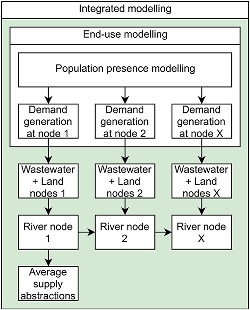
Figure 2. A generic illustration of the modelling domain for this study.

Development of CityWat-SemiDistributed Integrated Model

CWSD uses the physical representations presented in the CityWat integrated modelling framework and builds on the graph-based modelling philosophy exemplified by software such as CityDrain3 (Burger et al., 2016) to capture the spatial heterogeneity required for this study. A graph-based approach represents elements of interest as “nodes” that can be linked by “arcs.” Nodes do not have to be individual infrastructure works but can instead represent a strategic aggregation over an area (for example, a wastewater catchment) or over many works (for example, combining multiple river abstraction pumping stations). Arcs represent the flow of water; and are typically pipes or waterways. In CityDrain3 the graph formed by these nodes and arcs is “directed,” i.e., water flows from one node to the next in one direction, upstream to downstream. This can be thought of as “push-based” modelling, where each node pushes water to the next. Due to the importance of river abstractions on the River Thames, CWSD uses nodes that can both “push” and “pull” water along arcs. Push/pull modelling is common in the field of integrated modelling, and is the basis of many integration frameworks (e.g., OpenMI; Harpham et al., 2019). In this sense, the CWSD modelling philosophy adopts multiple model integration techniques and places them in a self-contained graph-based framework for simulation.

To expand the CityWat model from a lumped to a semi-distributed representation, we subdivided the area of interest into wastewater zones (each zone is a geographical area served by the same wastewater treatment plant, depicted in Figure 1) that can either be combined or separate sewer systems. The representation of surface runoff within each wastewater zone remained the same as in the original CityWat model, where the rational method was used to calculate the surface runoff and mass balance equations were used to calculate the flow (Dobson and Mijic, 2020b). In this study, to capture the spatial heterogeneities present in urban areas and to derive the runoff coefficients associated with each of the zones, we used a proprietary 2 m land cover dataset provided by the British Geological Survey. A wastewater zone's overall runoff coefficient was derived from first calculating the total amounts of each land cover class within the different zones and then applying the coefficient values presented in American Society of Civil Engineers and Water Pollution Control Federation (1986) to obtain the composite runoff coefficients. Other key physical assumptions relevant in this study that are also taken from the original CityWat model are instantaneous travel time of flows, representing sewer capacity with an “effective” drainage rate of 12 mm/h (based on Environment Agency guidance; Environment Agency, 2018) and a constant percentage reduction in pollutant concentration during treatment (described in section Integrated Modelling Over London Scale).

Alongside moving from a lumped to a semi-distributed representation, the most notable changes made to CityWat were around the representation of water quality. In the original study, water was considered to take one of three states: upstream river water, treated effluent and untreated sewage, and so to compare against measured water quality samples the model assumed each of the three states of water to have a fixed phosphorus concentration. In CWSD, due to the wide range of pollutants that exist in residential wastewater (Almeida et al., 1999), the concentration of a range of pollutants is tracked along arcs. Total pollutant concentration assumes well mixed conditions of river water, runoff, treated and untreated sewage. A sophisticated representation of biological, chemical, or fluid dynamical processes that influence pollutant concentrations was considered outside the scope of the study.

Integrated models of the environment are notoriously difficult to evaluate (Belete et al., 2017), particularly because performance of any specific sub-system is not necessarily indicative of the model as a whole (Voinov and Shugart, 2013). We believe that, until greater agreement has been reached around this issue, most applications of integrated models should be considered exploratory. With this in mind, a model evaluation is performed using openly available data (i.e., the WIMS database; Environment Agency, 2020) of pollutant concentrations. We do this on the basis that these variables should be the hardest to predict since they require high accuracy in both quantity and quality of all contributing processes within the model and also for the model boundaries. Instead of formal calibration, we select the values of the many parameters in the model based on data where possible and expert knowledge otherwise (described in Supplementary Material 1A–D, as are all parameters used in this study). The data used to do this are described in section Modelling Evaluation. Although calibration would likely provide higher “performance-metrics,” in a model so complex as presented in this study, there is no guarantee that the metrics would be improved for the “right reasons” (Kirchner, 2006). Since the purpose of the model in this study is for analysis of system changes under unprecedented conditions (i.e., COVID-19 scenarios), we favour potentially lower performance metrics but with defensible and transparent parameter values. We also acknowledge that the lack of formal model calibration limits the interpretation of results to inform operational decisions.

Stochastic Simulation of Water Demand

Simulating stochastic ensembles of water demand at scale can broadly be split into two required calculations, determining presence of the population in the area in question and then determining how much water they are consuming for different activities at a given time. We highlight the key steps in Figure 3.

FIGURE 3

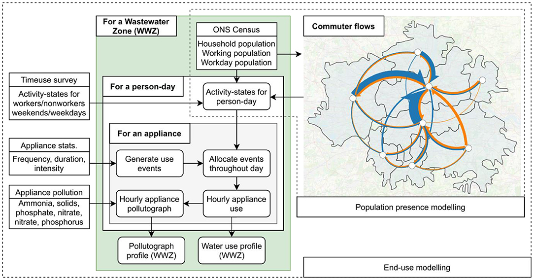
Figure 3. A flow chart demonstrating the key stages in the end-use modelling. The map depicts commuter flows between the eight wastewater zones in London. Flows with fewer than 5,000 people/day are not shown. Only commuting between zones is depicted for visibility, however commuting into/out of London is captured by the model. Arrow width is proportional to number of people per day, with the largest flow being 500,000 people/day. Arrows are coloured to highlight direction of flow.

A Population Presence Model for the UK

The key driver of household water consumption in an area is the total population. Census data are commonly used to inform household consumption in the context of wastewater (Blokker et al., 2010; Atinkpahoun et al., 2018). In addition, the UK census data is freely available anywhere in the UK (Office for National Statistics, 2011), and conducive toward reproducible research through the Office for National Statistics' API (Smith, 2017). Thus, census data is used to inform total household population, total number and size of households, and total population flows to/from an area due to commuting. Its high resolution enables accurate derivation of these values at a wastewater zone scale. The flow of commuters between different wastewater zones according to this census is displayed in Figure 3.

Although census data provides a reliable breakdown of the population in areas, it is a static view of the population (except for commuting numbers). The end-use modelling techniques described in the following section rely on within-day movements of the population, specifically determining when people are at home, away from home, asleep or at work (Blokker et al., 2010). To model behaviour in the baseline case (i.e., outside of COVID-19 scenarios) we use the “United Kingdom Time Use Survey 2014-2015” (Gershuny and Sullivan, 2017). For this survey, 11,000 randomly sampled people around the UK recorded their activities every 10 min for up to a week. While there are hundreds of different types of activity, we categorise them into four basic “activity states” to ensure each has a large sample size of associated timings. Following Blokker et al. (2010) these states are: sleep, home, away, work. Information about respondents such as region within the UK, employment status, household ownership, age, relationship status, education levels, and income are also included in the survey. Although many of these factors play a role in water use activity (Hussien et al., 2016), the relationship has not been quantified in a manner that would enable straightforward inclusion in our end-use model, thus we only account for employment status and region within the UK. The data also is further categorised based on “weekends” and “weekdays” for modelling purposes, since the time use patterns between the two are significantly different.

Pre-processing of census data provides population, worker and commuting numbers, while the time use survey provides respondent information in the region of interest. For each person in the wastewater zone, we sample a day from the time use survey. If the person is a worker (determined by the number of workers in the census survey) then we sample the day from an employed person in the survey, otherwise we sample a non-employed person. This will provide activity states at 10-min resolution for each person in the wastewater zone. Based on the commuting information in the census data, we split the workers into three groups: those who will be working and living in the wastewater zone, those who will be living in and working out of the zone and those who will only be working in the zone. For some cases, for example in central London where millions of people work, it is not computationally feasible to create presence information for each individual person; in these cases, we take as large a sample as possible and scale the information accordingly.

End-Use Modelling

End-use modelling describes a person or household's use of various appliances with statistical distributions and then uses Monte-Carlo simulation to derive a stochastic time-series of water demand. We use the appliances and activities presented in Blokker et al. (2010): baths, bathroom taps (washing and teeth brushing), dishwashers, kitchen taps (hand washing, dish washing, consumption), showering, washing machines, and toilet flushing. The key parameters to be estimated, typically via survey, are the frequency, intensity and duration of water consumption events. In this study, we use the parameters presented in Blokker et al. (2010), unless estimates that are tailored to the UK are available. These parameters and our sources for them are described in Supplementary Material 1C,D.

For each person-day, the number of events is generated, then, for each event, the intensity and duration are generated. These events are then distributed throughout the day and the location where water is consumed are based on the person's presence and activity-state, sleep/home/away/work (i.e., from section A Population Presence Model for the UK). Following Blokker et al. (2010), we assign a 1.5% probability of a given event occurring during the “sleep” activity-state, a 0% probability of occurring during the “away” activity-state and the remaining occurrences to occur during the “home” activity-state. If the person is a worker and working on a given day, the probability of using a toilet or bathroom tap at work is the same as at home (scaled in proportion to the number of hours at work/home). Finally, during the first morning period at home, there is an increased chance of using showers or bathroom taps such that there is a 50% probability that these occurrences take place during this period.

Our key motivation for using end-use modelling was its ability to link with the pollutant content of household effluent. There are a range of studies that document this information for specific water consuming activities (Almeida et al., 1999; Eriksson et al., 2002; Friedler, 2004; Li et al., 2009; Todt et al., 2015). These studies provided pollutant concentration estimates for chemical oxygen demand (COD), ammonia (NH₃), nitrite (NO₂), nitrate (NO₃), phosphate (PO₄), total phosphorus (P), and suspended solids (TSS), which are thus the pollutants we simulate in this work. The derivation of a pollutograph for total household effluent in CWSD is the proportional mixing of appliance pollutant concentration and appliance total flow, adding a novel application of the end-use modelling from a whole-water system perspective.

Integrated Modelling Over London Scale

The representation of London's urban water cycle used in CWSD is depicted in Figure 4. It captures all the significant inflows and abstractions from the River Thames and its tributaries using publicly available information ranging from 2004 to 2018. A detailed list of parameter values and sources can be found in Supplementary Material 1A,B. The spatial resolution for the model is river catchments (for inflow nodes), wastewater zones (for precipitation, demand, runoff, sewer networks, and wastewater treatment), and points (for river junctions and supply abstractions). The temporal resolution for the model is hourly to better capture time sensitive processes such as water consumption and runoff.

FIGURE 4

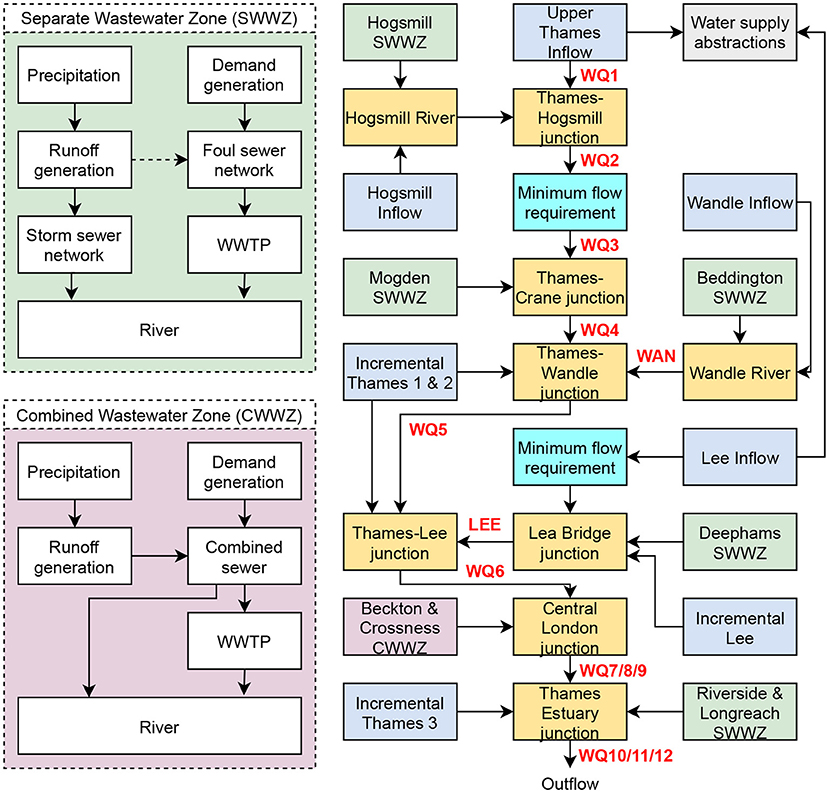
Figure 4. Schematic depicting nodes of the London model. Green nodes are separate wastewater zones, blue nodes are model inflows, gray is the water supply abstractions, orange nodes are junctions, cyan nodes are minimum flow requirements and purple is the two combined wastewater zones. WWTP stands for wastewater treatment plant. The dashed arrow in the Separate Wastewater Zone box (top left) represents infiltration into the foul sewer network. Water quality sampling sites are indicated in bold red and can be matched with the sites in Figure 1.

The two key data types used for the hourly forcing were river inflows and precipitation, with an overlap period of 2004-04-08 to 2018-09-30. Daily flow data was sourced from the National River Flow Archive (NRFA) (https://nrfa.ceh.ac.uk/, last accessed 2020-11-18) and hourly flow data for the Lee inflow and Thames inflow was obtained from the Environment Agency at 15-min resolution and processed to hourly. Incremental, Hogsmill and Wandle inflows each had suitable gauging stations from the NRFA to provide daily flows. These daily flows were downscaled to hourly by scaling from the Lee or Thames hourly flow data.

A weather radar product was used to create hourly precipitation forcing. The data is a radar composite from the operational C-band network of the UK Met Office (Met Office, 2003). The original resolution of the radar product is 1 km at 5-min intervals. The product has been post-processed and quality controlled by incorporating rain gauge data (Harrison et al., 2012). In the radar Quantitative Precipitation Estimation (QPE), a range of estimation errors still exist, related to ground clutter, beam blocking, bright band, and conversion between reflectivity and rain rate. However, for the study area, the radar QPE has shown to give a good estimation of annual precipitation (Fairman et al., 2015, Figure 5) and a more realistic diurnal pattern than other observation datasets (Fosser et al., 2020). To obtain the time series representing the areal rainfall observation in each wastewater zone, we spatially averaged the radar measurement covering the zone and then aggregated data to hourly. When more than 50% of data shows missing or abnormal in an averaging or aggregation, we performed a linear interpolation between adjacent timesteps.

FIGURE 5

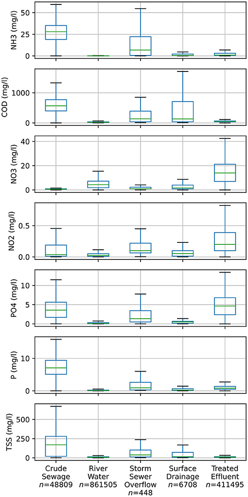
Figure 5. The pollution content of every sample in the WIMS database, sorted by sample material (i.e., each column) for the pollutants considered in this study (each pollutant is a row). Green bars indicate the median value, boxes the interquartile range (IQR) and whiskers indicate the range of measurements that are ± IQR*1.5 within the upper and lower quartiles. Measurements that fall outside of the whiskers are not shown to improve the readability of plots. The average number of samples across the presented pollutants is indicated for each sample material by “n”.

While pollutant concentration is produced as an output of the end-use modelling, a method was required to determine concentrations for inflow nodes and runoff generation, for which we used the WIMS database (Environment Agency, 2020). This database is a collection of Environment Agency water quality samples between 2000 and 2020. In Figure 5, we summarise the distribution of sample results for the pollutants used in our study across all samples in the database (i.e., that cover all of England), further sub-divided for each type of water that is being sampled (referred to as “sample material”) within each panel. The sample materials we depict here are: crude sewage, treated effluent, river water, storm sewer overflow discharge, and surface drainage. To create hourly forcing we performed linear interpolation between sample values at sampling sites near the river gauges that we used for streamflow. The frequency of samples for inflow points ranged between weekly and monthly, however the sampling periods did not generally cover the entire simulation period (2004-2018). We have extrapolated outside the sampled periods using the mean concentration for each pollutant at a given site. Although rivers are relatively well sampled in the database (with on average 850,000 measurements per pollutant nationwide), surface drainage is not (with only 7,000 measurements). Due to this scarcity of samples, we set surface drainage pollutant concentrations to the median values displayed in the fourth column of Figure 5. Because we envisage this summary of pollutant concentrations by sample material may be useful, we provide a table with more detailed statistics and a greater number of pollutant types in Supplemental Material 2.

As observed in previous studies (Almeida et al., 1999), in-sewer biological and chemical processes mean that the pollutant concentrations in household wastewater are significantly different from the sewage that reaches wastewater treatment plants. For example, the range of concentration in nitrate from the end-use generator is between 3 and 5 mg/l, while the concentrations in crude sewage seen in Figure 5 are closer to 0.6 mg/l (these values are similar to those reported in Almeida et al., 1999). To avoid further increasing the model complexity, we apply a linear correction factor on pollutant concentrations in sewers to account for these processes. We also use the concentration change between crude sewage and treated effluent in Figure 5 to inform the percentage reduction of each pollutant that takes place during the treatment process.

The ultimate purpose of the integrated modelling work in this study was to model changes in the urban water cycle that may occur under COVID-19, facilitated by the population presence and end-use modelling of water consumption. No data yet exists on changes in London's population due to COVID-19, nor what long lasting changes the pandemic may have had on it. Instead, we create three “hypothetical” scenarios to capture different types of impact:

• Work from home (WH). In this scenario, the number of people who follow “employed” time use patterns is reduced by 90%. Those people instead follow “non-employed” time use patterns and no longer commute to their work destinations.

• Lockdown (LD). Same as work from home, but all activity-states of “away from home” are set to “at home.”

• Population decrease (PD). The population of each zone is reduced by 15%, reflecting the potential movement out of London notionally reported in Wilson (2020). We model population changes at this citywide scale due to a lack of up-to-date information.

Modelling Evaluation

Evaluation of Integrated Modelling

As described in section Development of CityWat-SemiDistributed Integrated Model, we calculate performance metrics by comparing simulated pollutant concentrations against water quality data. The WIMS database contains both in-river samples and crude sewage samples at some of the WWTPs. Because the precise time at which samples are taken is recorded in WIMS, but the CWSD is run at an hourly timestep, we round WIMS sample time to the nearest hour to compare samples with model predictions. Following literature that compares simulated water quality against relatively sparse pollutant samples (Jackson-Blake et al., 2017), we evaluate the model using percentage bias, Nash-Sutcliffe efficiency and Spearman rank. We also provide plots that show simulation data against WIMS samples to highlight the complexity of validating integrated models of the urban water cycle.

River flow data from the WIMS archive is available for 2020, however it has a dramatically reduced sampling frequency; around a tenth of the 2000-2019 average rate for the same period. Disentangling so few samples from hydrological variability would not be possible for an informative comparison. Thus, we instead simulate these scenarios for the period of overlapping data (i.e., 2004-2018). This longer simulation period will also reduce the impact of hydrological and climate variability on results, ensuring that they are attributable to COVID-19 scenario choice only. We base our discussion on simulations of mean relative change in flows and pollutant concentrations for model arcs under each scenario.

Evaluation of End-Use Modelling

Because the end-use model presented in this study is a separate contribution, we provide an application to evaluate it. This application uses hourly metered household data from both before and during the COVID-19 pandemic. We test the end-use model in 11 separate supply distribution zones in a combination of rural villages and towns in England, assuming that a model evaluation in these areas can be representative across the UK. The population of each zone ranges from 200 to 9,000. The metre data consists of >400 million automated hourly readings. A basic pre-processing step is performed to remove readings that are not reflective of the household consumption patterns that this study aims to capture (i.e., zero variability in readings, zero consumption over record, measurements that are >10x a household's median consumption). We also remove non-domestic properties since the end-use model is intended for household water consumption only. Because this metre data is proprietry, we cannot share further information about it.

We run the end-use model using both normal settings and the “work from home” scenario described. From the model outputs we compare the mean per-capita diurnal consumption profile for each zone against metre data. We compare against the diurnal profile because the end-use model is stochastic, and so it would not be logical to compare against individual metre readings. We measure the performance using NSE values.

Results

Modelling Evaluation

In this section we provide a relevant selection of simulation results against available data. Integrated modelling evaluation results are presented in full and examined in detail in Appendix 1, where we compare the model simulations of water quality over the historic period with in-river water quality samples. Demand modelling evaluation results are presented in full in Appendix 2, where we compare end-use modelling generated demand profiles with metered data both before and during the COVID-19 pandemic.

Figure 6 demonstrates the mean percentage bias between CWSD simulated and WIMS sampled water quality data at wastewater effluent sampling sites and in-river sampling sites. We present percentage bias here because we examine the mean change in pollutant concentrations between the baseline and COVID-19 scenarios in section Analysis of London's Water System Under COVID-19, however NSE and SR are presented in Table A1, Appendix 1. In general Figure 6 shows better predictions in the tributaries and more upstream locations in the River Thames, while the two most downstream sites (two rightmost columns) are the hardest locations to predict. Suspended solids (top row) is overpredicted in tributaries and underpredicted in all sites in the River Thames except the most upstream. Phosphates, nitrites, and nitrates are overpredicted in treated effluent but slightly underpredicted in rivers. Ammonia is generally overpredicted at treatment plants, except for Longreach and Crossness where it is underpredicted (the WIMS samples for effluent at these plants has significantly higher ammonia concentrations than others). Meanwhile, phosphorus is underpredicted at all treatment plants except Deephams and Hogsmill (again, different plants produce significantly different concentrations of phosphorus in the WIMS sample database but not in CWSD).

FIGURE 6

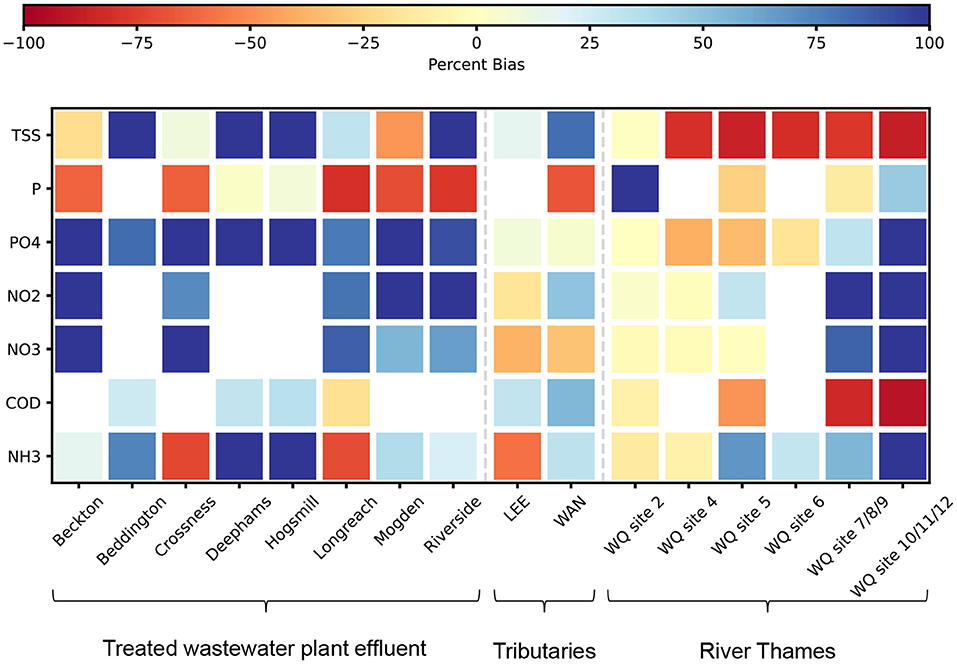
Figure 6. Percentage bias metric between simulated and sampled water quality values for treated effluent arcs (left side), in-river arcs for tributaries to the River Thames (central) and in-river arcs for the River Thames (right side). Cells that have been left blank have no recorded water quality samples. Values with a percent bias greater than ± 100% have been set to 100 to improve the visual interpretation of the plot. Locations for arcs can be matched to Figures 1, 4.

In Appendix 1, Figure A1 we plot a selection of simulated data and compare against in-river water quality samples to highlight difficulties in integrated modelling. Figure A1A shows phosphate concentrations in a tributary, highlighting that, although projections look qualitatively accurate, performance metrics do not reflect this due to the high intra-day variability in concentrations. Figure A1B plots suspended solids concentrations at a water treatment plant, demonstrating that the variability of samples is outside what is achievable by the model, indicating that the model is missing some key process(es), presumably in urban runoff or treatment plant representation. Chemical oxygen demand in a tributary, Figure A1C, shows how sampled “peaks” can be delayed from the simulated peaks, thus highlighting the impact of assuming instantaneous water travel-time in the model. Phosphate concentration at a treatment plant, Figure A1D, shows a consistent bias in simulations that is likely caused by parameter choices, however it is not clear whether parameters for phosphate influent levels or in treatment plant processes (or a combination) are responsible for the bias.

To characterise the performance of the demand modelling results, we present a plot (Figure 7) that shows the simulated hourly diurnal consumption profile (solid lines) in comparison to the metered consumption profile (dashed lines) for both weekdays (cyan) and weekends (magenta) for a metered area. This metered area was selected for display because it was the most populous of the available zones (with around 10,000 people). The modelling results show good agreement in general, with a NSE of 0.94 for weekdays and 0.89 for weekends. We see a “too-sharp” morning peak on weekdays, and a “too-low” morning peak on weekends – these deficiencies are common to all zones. As we demonstrate in Table A2, the method performs effectively for all metered areas and also during the COVID-19 lockdown.

FIGURE 7

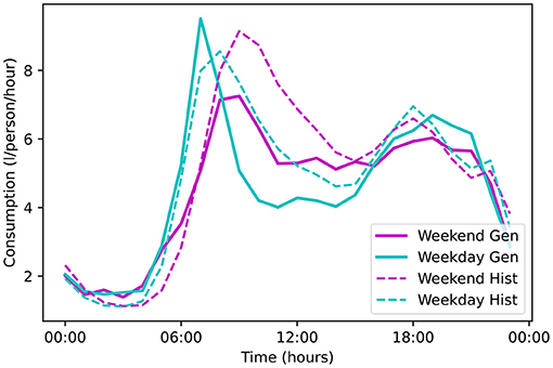
Figure 7. The hourly per capita diurnal water consumption profile for the most populous metered area in the survey. (Solid lines) Average water consumption for a given hour from the generator on weekdays (cyan) and weekends (magenta). (Dashed lines) Average water consumption for a given hour from the metre survey on weekdays (cyan) and weekends (magenta).

Analysis of London's Water System Under COVID-19

Changes in Population and Water Consumption

We show the wastewater zone scale changes to daily population that result from a 90% decrease in commuting (i.e., the population shift in both the lockdown and work from home scenarios) in Figure 8A. The central London wastewater zone (Beckton) experiences a 23% decrease in average weekday population and 10% decrease in average weekend population. This is a result of nearly 1 million commuters no longer travelling to and working in the area. In all other zones the reduction in commuting increases the population by between 4 and 10% for weekdays and 1–3% for weekends.

FIGURE 8

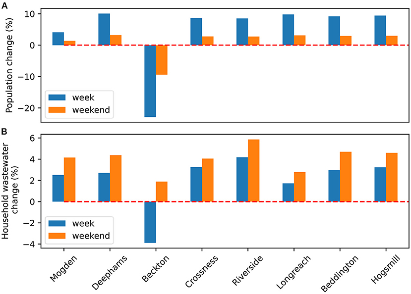
Figure 8. Population change during lockdown (A) and household wastewater flow change (B) on weekdays and weekends. Changes are the relative difference between the baseline scenario and lockdown scenario. Zero change is marked by the dashed red line.

Figure 8B shows changes in household water consumption that are being driven by two key mechanisms: changing population and time-use dynamics. The changing population impact is apparent in the Beckton zone, with its reduced wastewater production on weekdays. However, the reduction in wastewater is smaller than the reduction in population because the only significant water consumption activity at work is toilet flushing. For example, in the Beckton wastewater zone 12% of daily water consumption comes from workplace toilet flushing. Because 50% of the workplace population in Beckton are commuting from outside of the zone, a 90% decrease in office working will reduce total consumption by only 5%. Meanwhile, the time-use dynamics mechanisms are evident in a weekend-weekday comparison; observing that most zones have a larger increase in population on weekdays than weekends, but an opposite pattern with respect to wastewater flows. This occurs because people typically spend more time away from home on weekends than weekdays under normal conditions, leading to a larger relative in increase time spent at home on weekends due to lockdown. This greater amount of time spent at home translates into more time to perform water consuming activities and thus a larger relative impact of lockdown on weekends than weekdays that outweighs the population change pattern.

To provide a more detailed insight, we plot the change in diurnal water consumption profiles under lockdown, working from home and the population decrease scenarios in Figure 9. In Figures 9A,B we show the changes in the central London wastewater zone (Beckton) because it is the most populous zone containing London's central business districts. Due to the reduction in work-place toilet flushing from fewer commuters, the work from home scenario experiences a significant decrease in consumption during working hours of weekdays compared to baseline. The profile looks significantly different in the lockdown scenario because there are minimal work or other house-leaving activities to introduce variability in water consumption, resulting in the relatively constant consumption throughout the day. As expected, the population decrease scenario translates the profile to a reduced level of water use. To contrast against central London, we plot a more suburban wastewater zone (Hogsmill) in Figures 9C,D. This zone follows similar trends except for the work from home scenario in Figure 9C, where there is a slight increase during working hours rather than the large decrease that is seen in Beckton.

FIGURE 9

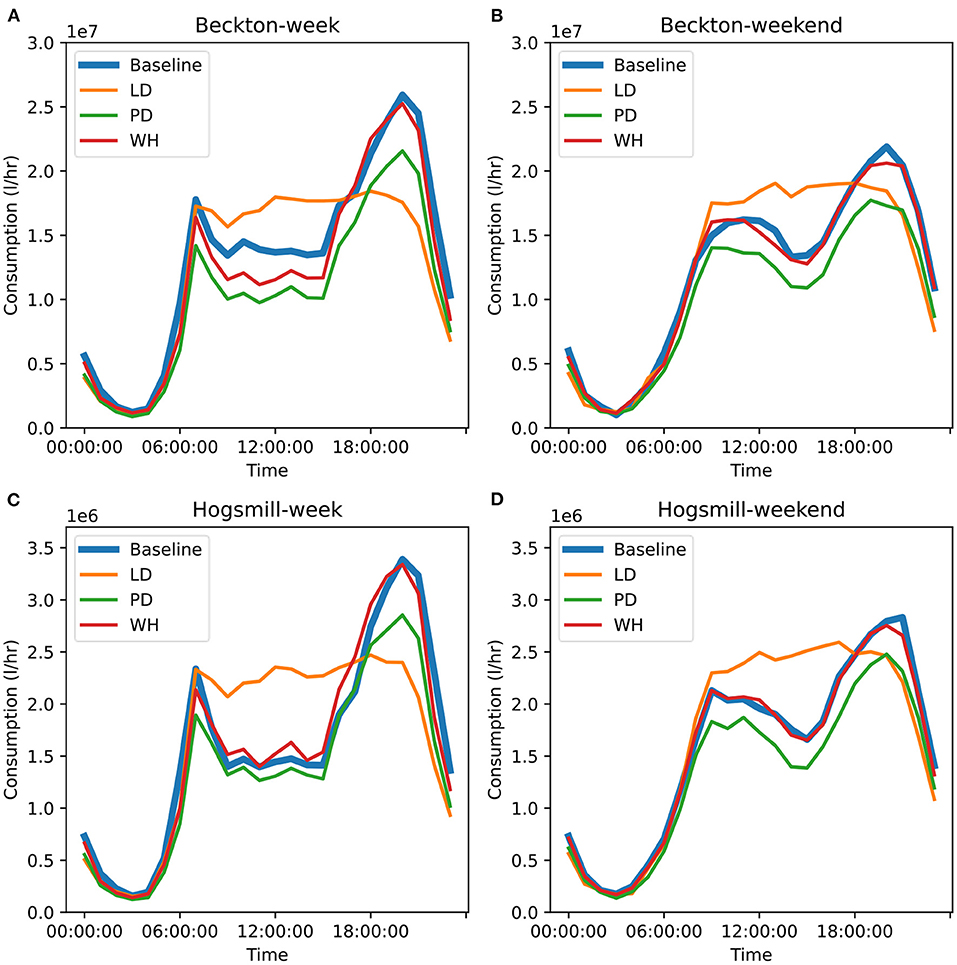
Figure 9. Change in daily consumption profile in the Beckton wastewater zone (A,B), and Hogsmill wastewater zone (C,D), for both weekdays (A,C) and weekends (B,D). Blue is baseline, orange is lockdown (LD), green is the population decrease (PD) scenario, red is work from home (WH).

Changes in Water Quality Throughout Integrated Water System

We have investigated changes at five points throughout the urban water cycle, including household waste, treated effluent, untreated sewage spills, and in-river concentrations.

In Figure 10 we plot the percentage change between pollutants and flow for each wastewater zone's household waste for each scenario. The most significant differences are in the Beckton wastewater zone. This can largely be attributed to the significant decrease in effluent that is made up by toilet flushing from the “missing” commuter population (i.e., the 20% daily population reduction seen in Figure 8). As noted in the previous section, this reduction in flushing does not significantly decrease the total effluent. However, because flushing is the primary source of ammonia and solids, we see a significant decrease in these concentrations. We also see an increase in nitrate and nitrite concentrations, which is because flushing has low concentrations of these pollutants and as flushing decreases it no longer dilutes the other household activities. Other zones have far smaller changes because their daily population changes due to commuting are proportionally smaller. In general, there is a slight increase in flow during lockdown not seen during the work from home scenario – this is because people spend significantly more time at home and have a greater chance to perform water consuming activities. The population decrease scenario expectedly decreases flows in each zone, albeit not uniformly because commuter patterns remain unchanged in this scenario. Increases in nitrite concentration in zones other than Beckton under the population decrease scenario are seen because the primary source of nitrite is from kitchen taps, which are more strongly tied to the number of households than total population. Thus, population decrease reduces other water consumption activities more quickly than kitchen tap usage.

FIGURE 10

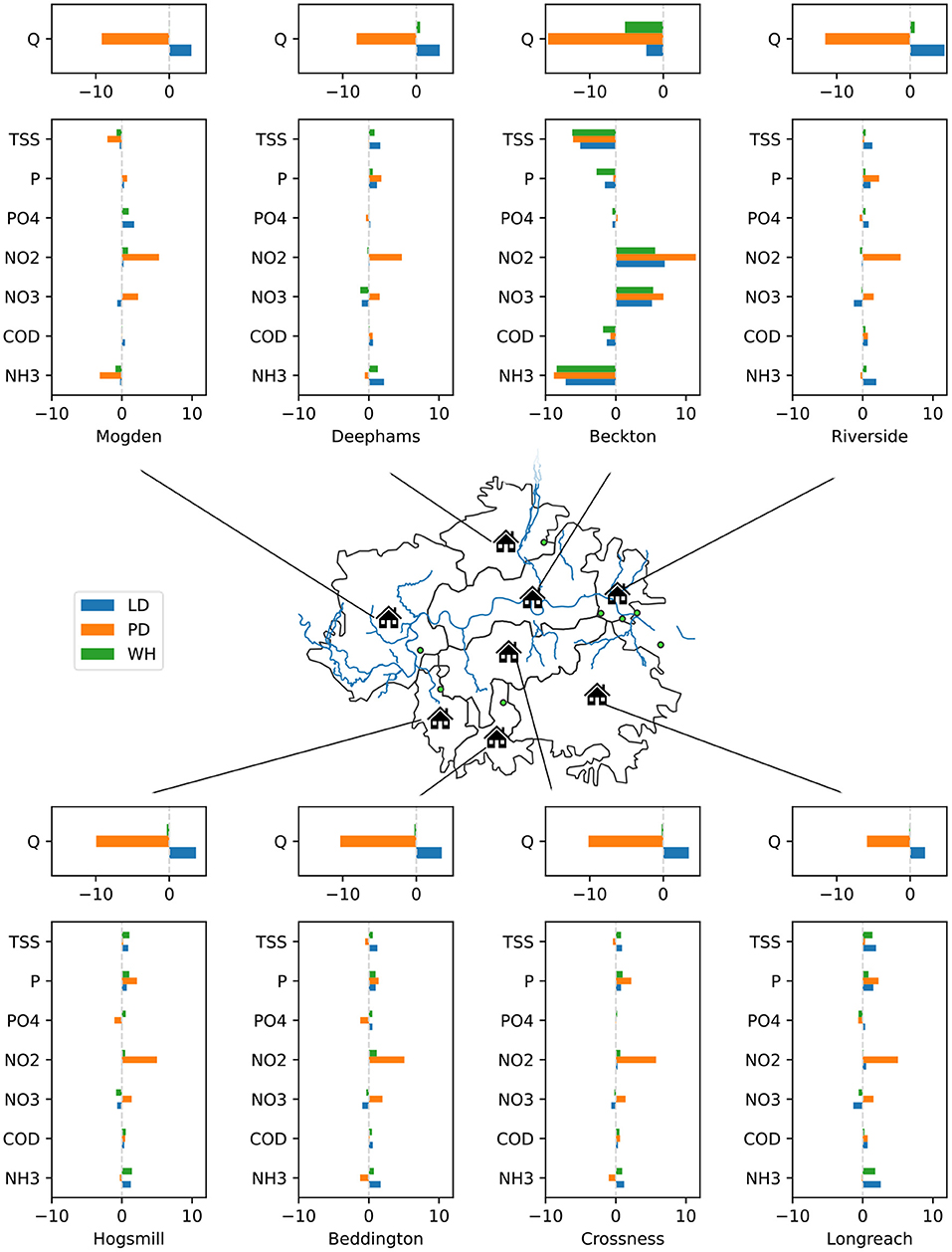
Figure 10. Map depicting percentage changes in household wastewater flow and pollutant concentration (these are the bars). LD stands for the lockdown scenario, PD stands for the population decrease scenario and WH stands for the work from home scenario.

To understand how these changes in effluent and pollutant concentration propagate through the water cycle, we show changes to treated effluent from wastewater treatment works in Supplementary Figure 1 in Supplementary Material 3. We do not present this in the main text because the patterns shown in Supplementary Figure 1 are similar to Figure 10, with only small changes resulting from surface runoff that is eventually treated and differences in how effectively different pollutants can be treated. The magnitude of differences for flows in Figure 10 are smaller than Supplementary Figure 1 due to surface runoff. The magnitude of differences for pollutants in Figure 10 are generally the same as in Supplementary Figure 1, except for the Beckton wastewater zone, which treats a greater proportion of rainfall than the other zones.

When treatment plants and their stormwater storage or combined sewer systems are at capacity, they are forced to spill untreated sewage directly into rivers. The changes during the COVID-19 scenarios are presented in Supplementary Figure 2 in Supplementary Material 3. We present this in the supplementary material because, besides those described below, there are minimal differences between different wastewater zones. We find minimal changes in the flow of these spills because these events are primarily driven by high precipitation and so population changes have little impact. However, household wastewater is still a primary source of some pollutants in these spills and so changes in household water consumption will impact pollutant concentrations. In the Beckton wastewater zone we find decreasing concentrations of suspended solids, phosphorus, phosphate, and ammonia for all scenarios due to the decreased population. Meanwhile, the other wastewater zones see decreases in concentration for the population decrease scenario and increases for the work from home and lockdown scenarios, again reflecting the changes in population. Nitrates, nitrites, and COD do not significantly change for any zones/scenarios because these pollutants are not significantly lower in surface runoff than they are in household waste.

Finally, in Figure 11 we show the changes in river quality, since ensuring a high level of environmental performance is one of the key motivations for integrated water cycle modelling. Changes, in general, are minimal, reflecting the significant role of the natural environment in regulating ecosystem services through the dilution capacity of rivers. Ammonia and phosphate are the variables most sensitive to the different scenarios, with nitrite to a lesser extent. This is because the concentrations of these pollutants are typically very low in natural rivers, with wastewater effluent being the main source of pollution. We can observe this in Figure 5, noting that these variables experience the largest difference between concentration in “treated effluent” and in “river water.” In Figure 11 we also see that the smaller tributaries to the River Thames (River Lee and River Wandle) are the most sensitive to the lockdown scenario, due to having less water to dilute the additional pollutants, with potentially significant implications for quality of environment for local residents.

FIGURE 11

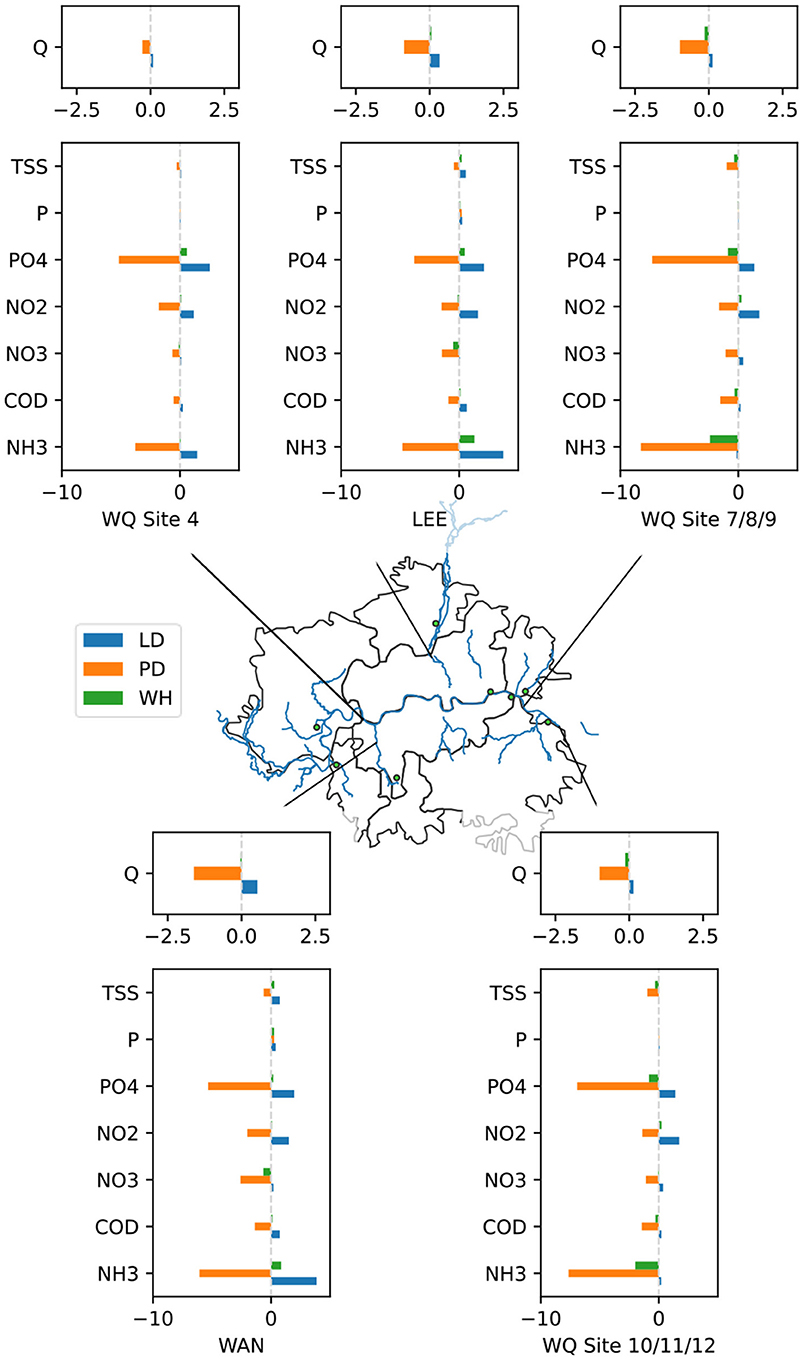
Figure 11. Map depicting percentage changes in river flow and pollutant concentration (these are the bars). LD stands for the lockdown scenario, PD stands for the population decrease scenario and WH stands for the work from home scenario.

Discussion

This study aimed to provide three key contributions; the first was expanding an existing integrated urban water cycle model to provide a more detailed spatial perspective. Figures 10, 11 and Supplementary Figures 1, 2 demonstrate how such a model can trace pollutants through the water cycle. The spatial perspective provides a range of benefits, for example quantifying the vulnerability of smaller rivers to changes and highlighting the importance of dilution for in-river pollution management (Figure 11). The in-river modelling capabilities highlighted how pollutants that increased most in the discharges from households (nitrites and nitrates in Figure 10) were not necessarily those that increased the most in rivers (ammonia and phosphate in Figure 11). This is due to the relatively high concentrations of nitrates/nitrites and low concentrations of ammonia/phosphate that occur naturally in rivers. These results could be particularly relevant for environmental regulators, water companies and NGOs, who could use the information to design targeted mitigation measures to deal with either local pollution or specific critical pollutants.

The second contribution was to create an end-use household consumption model that could easily be applied at large scales to any location in the UK by linking with census data and a national time use survey. Table A2 and Figure 7 demonstrated that the presented method worked effectively both before and during the COVID-19 period. Figure 8 indicated how, despite the dramatic changes in population that resulted from a lockdown scenario, changes in actual household consumption for London were not as substantial as might be anticipated and were driven not just by spatial redistribution of population but also by changes in time-use dynamics imposed by lockdown. This finding was only possible with an end-use model that separates appliance usage from households and workplaces. We believe this shows how an over-focus on statistical and data-driven approaches present in the demand forecasting literature (e.g., Donkor et al., 2014) may risk leading planners astray by missing the fundamental drivers of water demand. Future work may seek to inform COVID-19 scenarios by state-of-the-art in population-presence modelling, such as using mobile network traffic data (Khodabandelou et al., 2016), or to account for seasonal climatic sensitivities by explicit representations of outdoor spaces (Fox et al., 2009). Meanwhile, further developments in modelling non-household water demand (e.g., from industry) would be required for a more “complete” representation of urban water demand (Melville-Shreeve et al., 2021).

The ultimate goal of this study was to understand how water quality in London's urban water cycle may be changing due to mobility restrictions under emergency circumstances, such as COVID-19. Figure 9 shows how a lockdown scenario may cause sustained demand throughout the day and result in higher overall demand due to more time to perform water consuming activities. Figure 10 and Supplementary Figure 1 show that this will change the concentration of pollutants in places where commuters reside and where they work. These changes are not necessarily obvious without end-use modelling, for example Figure 10 shows that the decrease in toilet flushing will decrease ammonia and suspended solids concentrations but increase nitrate and nitrate concentrations up to 10%. The overall impact on in-river quality (Figure 11) shows a small but significant rise in ammonia and phosphate in the lockdown scenario on the Lee and Wandle (tributaries of the River Thames). Meanwhile, the population decrease scenario, which may be closer to what is happening based on anecdotal information, resulted in almost entirely positive impacts on in-river quality. These results are in line with other COVID-19 impact studies that generally report positive impacts on water quality (Braga et al., 2020; Hallema et al., 2020). A move towards a greater percentage of people working from home, which may be a longer-term outcome of the crisis, appears to have the least impact on London's rivers of all three investigated scenarios. Although this seems broadly positive, the authors caution that a possible resulting migration away from cities is likely to stress water infrastructures and potentially rivers by swelling the population of areas that are unprepared to cope with greater amounts of household consumption.

It is clear that the performance metrics presented in Figure 6 and Appendix 1 could have been improved through calibration of parameters. For example, the model underestimates the COD reduction that occurs at Deephams wastewater treatment plant (Figure A1C), while it overestimates the phosphates produced in the Longreach wastewater catchment (Figure A1D). However, we believe that changing these parameters without a basis for doing so runs the risk of creating seemingly accurate predictions that do not reflect reality (Kirchner, 2006). For example, any parametric correction that improves predictions seen in Figure A1B is likely to be artificial, and instead should be addressed by a more sophisticated representation of the land runoff and wastewater treatment processes. The model's application for detailed impact assessment or design is limited by sparcity of data available for evaluation, which is a common issue in integrated water cycle modelling (Belete et al., 2017). Thus, we have ensured results are interpreted at a high-level and are focused on the relative differences between scenarios. Having more accurate and spatially distributed data, in this case on water demand and the river water quality, would contribute to a stronger evaluation of the model simulations. This makes the dramatic reduction in water quality sampling observed in the WIMS database (a 90 percent reduction at sampling sites around England) all the more worrying; at times when the dynamics of the urban water cycle are most likely to be changing, we are collecting the fewest samples.

The future of integrated modelling of the urban water cycle lies in identifying where and why predictions are poor, and then finding ways to improve them and quantify their accuracy. Use of detailed physical models may provide insight about sub-systems' (e.g., wastewater network) behaviours, which can then be used to improve the representation of processes in an integrated model (Thrysøe et al., 2019). Accurate representations of human processes (e.g., river abstractions) will require working with stakeholders, including water companies, local authorities and citizens, to improve understanding and create better solutions for urban water management. Finally, as demonstrated by parsimonious water quality models performing similarly to more complex ones (Jackson-Blake et al., 2017), the question remains what the optimal balance between the model complexity, computational efficiency and accuracy is to support integrated water planning decisions.

Concluding Remarks

This study has demonstrated that integrated modelling of the urban water cycle in a spatially explicit manner is possible and necessary to provide evidence on the implications of unprecedented societal disruptions such as COVID-19. We find that the tributaries to the River Thames are more vulnerable than the Thames itself to potential changes that may have occurred under the COVID-19 anti-contagion measures, highlighting the important role that rivers play in diluting effluent. While more work is needed to ensure the accuracy of CWSD so that results can be used to inform operational decisions, it is clear that integrated modelling has great potential to profoundly change the way we plan and manage the urban water cycle. Such a tool may facilitate more seamless management of pollutants to better coordinate between water companies and environmental regulators, enabling them to “optimise for river quality” and determine the “hotspots” where placement monitoring equipment might provide the best value for information.

Data Availability Statement

The datasets generated for this study can be found in online repositories. The names of the repository/repositories and accession number(s) can be found in the article/Supplementary Material. The integrated modelling code and data used in this work is available at 10.5281/zenodo.4315110. The metre data used to evaluate end-use modelling is not available due to privacy concerns.

Author Contributions

BD and AM performed the demand modelling and integration framework. TJ performed the land use and runoff processing/modelling. YC performed the precipitation processing/modelling. AM, AP, and AB provided scope and discussion around COVID-19 impacts. All authors contributed to the manuscript writing and plots.

Funding

The research reported in this paper was taken as part of the CAMELLIA project (Community Water Management for a Liveable London), funded by the Natural Environment Research Council (NERC) under grant NE/S003495/1.

Disclaimer

The views expressed in this paper are those of the authors alone, and not the organisations for which they work.

Conflict of Interest

The authors declare that the research was conducted in the absence of any commercial or financial relationships that could be construed as a potential conflict of interest.

The reviewer SG declared a past co-authorship with one of the authors AM to the handling editor.

Acknowledgments

The authors are grateful to Gemma Coxon, University of Bristol, for providing the hourly river flow data used in this study. We also thank two reviewers and editor Boris M. Van Breukelen for their constructive comments that have improved the paper.

Supplementary Material

The Supplementary Material for this article can be found online at: https://www.frontiersin.org/articles/10.3389/frwa.2021.641462/full#supplementary-material

References

Almeida, M. C., Butler, D., and Friedler, E. (1999). At-source domestic wastewater quality. Urban Water 1, 49–55. doi: 10.1016/s1462-0758(99)00008-4