Global Solar Magnetic Field Evolution Over 4 Solar Cycles: Use of the McIntosh Archive

Introduction

Science Objectives

The magnetic field of the Sun is driven by its dynamo generated in the solar interior which emerges through its surface, and ultimately permeates the heliosphere. The evolution of this field is manifested in large-scale surface features such as filaments, active regions and sunspots, polarity boundaries, and coronal holes (CHs). Ongoing surface diffusion and transport yields an evolving pattern of positive and negative magnetic polarity regions that comprise the global magnetic field. Over solar-cycle (SC) time scales, these motions can help us understand the internal fluid dynamics of the Sun.

The Sun exhibits a few characteristic migration patterns of surface features. One is the equatorward movement of the latitude zone of sunspots, a fundamental feature of the 11-year activity cycle. Another is the movement toward the poles of high-latitude filaments/prominences and their related unipolar magnetic regions (UMRs). This involves the so-called “rush-to-the-poles,” a tracer of the solar polarity reversal process and the onset of the 22-year magnetic cycle (Babcock, 1961; Leighton, 1964, 1969). These migrations are also associated with zonal surface or near-surface flows such as torsional oscillations.

Recent observations of sunspots and other small-scale magnetic features (e.g., McIntosh et al., 2014; McIntosh et al., under review), as well as helioseismic studies of zonal flows (Howe, 2016) provide support for an “extended” cycle of solar activity (Cliver, 2014), e.g., from 17 to 22 years long. In addition, the polar field strength at activity minimum has been used to predict the following cycle's sunspot number peak (e.g., Munoz-Jarmillo et al., 2013). It is clear that observing the evolution of such surface features over long, SC-time scales is important for understanding the internal fluid dynamics of the Sun.

The overall science objective which is enabled by the newly processed McIntosh Archive (McA) maps is to investigate the long-term variability of solar surface features. Our work highlights understanding the sources and evolution of active regions, CHs, filaments and PILs, how the rotation rates of these features vary over SCs, and the long-term variation of the toroidal and poloidal components of the magnetic field and their connection to the interior dynamo (see also Webb et al., 2017).

History and Preservation¹

Toward this objective in 1964 during SC 20, Patrick McIntosh began making hand-drawn synoptic maps of solar activity, based initially on daily Hα images (Figure 1, top). These maps were unique in that they traced the polarity inversion lines (PILs, or neutral lines) that connected widely separated filaments, fibril patterns and active region corridors to disclose the large-scale pattern of the global magnetic field. In that epoch magnetographs were expensive, less reliable, and their magnetograms were not available on a routine basis. For example, H. Babcock and colleagues at Mount Wilson Observatory started relatively routine magnetograph observations beginning in 1959, however, these data were not available in digital format. Another advantage of using Hα images was that PILs could be more accurately tracked through weak-field regions and near the solar poles (e.g., Fox et al., 1998; McIntosh, 2003). McIntosh (1979) and others showed that the large-scale Hα surface patterns matched well with the large-scale magnetic fields and their boundaries as measured on magnetographs.

FIGURE 1

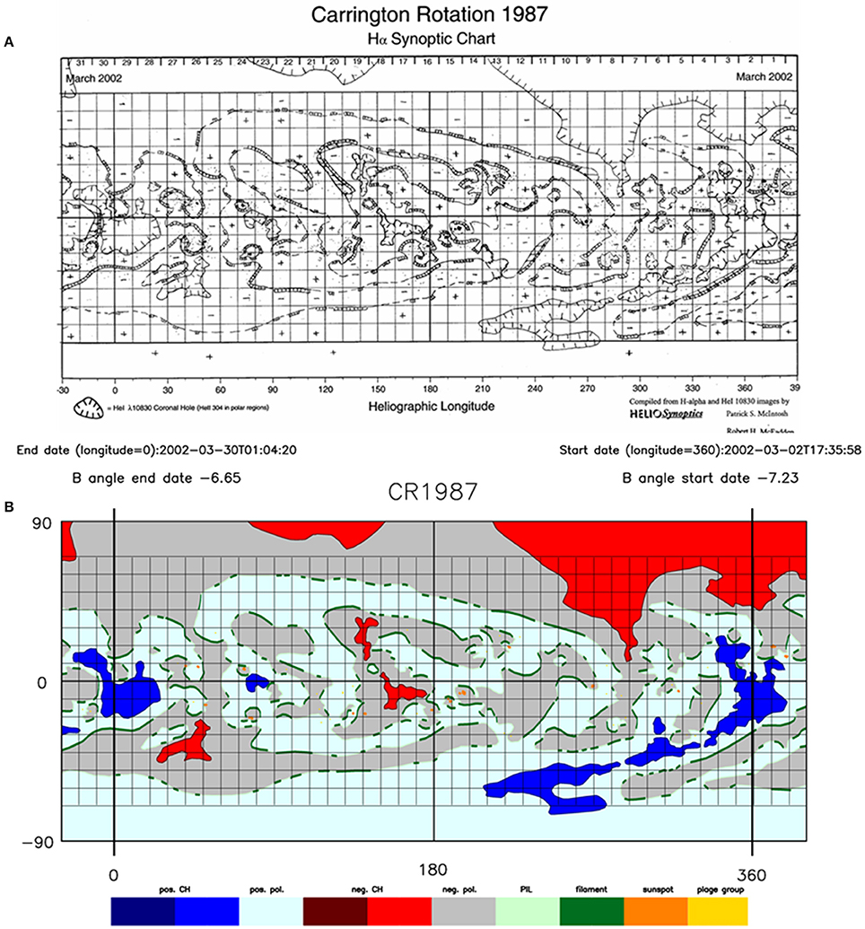
Figure 1. (A) Scanned image (Level 0) of an original synoptic map in from March 2002 created by Pat McIntosh. (B) Processed colorized map (Level 3) from the new McIntosh archive with negative (gray) and positive (white) polarity magnetic fields, negative (red) and positive (blue) CHs, filaments (green), and PILs (black). The Supplementary Material contains movies of the full McA of the original synoptic maps (Level 1; Movie 1) and of the final processed maps (Level3; Movie 2).

Beginning in 1981, CHs were routinely added to the maps, primarily from ground-based He-I 10830 Å images from NSO-Kitt Peak. When available, magnetograms were used to determine the overall dominant magnetic polarities and to show where their boundaries were. Many of the original hand-drawn McIntosh maps were published as Upper Atmosphere Geophysics (UAG) reports: McIntosh (1975; May 1973–March 1974), McIntosh and Nolte (1975; October 1964-August 1965), and McIntosh (1979; 1964-1974). The maps were also routinely published in the Solar-Geophysical Data (SGD) Bulletins (the “Yellow books”). All of these reports are archived at the NOAA National Center for Environmental Information (NCEI).

McIntosh and various assistants generated these maps for each Carrington Rotation (CR) from 1964 to 2009, with some gaps including a 2-year period from July 1974-July 1976. This 45-year period covers four complete SCs, or 600 CRs. The features on the maps include filaments, sunspots and active regions, large-scale positive and negative polarity regions, and CHs of each polarity (Figure 1, top). The McA is distinctive in providing a long-term, reliable view of the evolution of the global solar field.

In a study that is done over such a long period, it is clear that there will be changes in personnel and advances in technology, technique and equipment. For example, we recognize that the coronal hole boundary data gathered by Skylab in 1973 and 1974 in the He-II line differs somewhat from that in He-l that we switched to in 1974 from Kitt Peak. Over the 45 years that the original maps were made, having a consistent high quality of the images used, especially Hα, was considered more important than the consistency of using the same observatory. However, consistency of observatory was not ignored. Only when the preferred observatory's data was not available was an alternative chosen. Of course all data were adjusted for time and, therefore, longitudinal differences.

Pat McIntosh is deceased (Hewins et al., 2017), but his assistants coauthors I. Hewins and R. McFadden were trained by Pat in how to produce the maps. However, after Pat became disabled then died, the maps and related materials were kept in boxes and scattered among various homes and basements. In addition, none of the scanned maps were suitable for digital analyses. The first and foremost intent of the McA project was to preserve the entire archive. This has been achieved by collecting and collating all of the material at the High Altitude Observatory (HAO) in Boulder, CO and completing scanning of all of the maps in a uniform manner.

The metadata is very comprehensive with the observatories and original cartographers recorded for each of the maps. We emphasize that Pat McIntosh taught all the assistants the technique and trained them for about 6 months before they were ready to contribute to any final products. Even after this training, McIntosh still reviewed, and where necessary modified the synoptic maps until he had a final product he was satisfied with. Thus, McIntosh created, worked on or reviewed all of the maps in the archive. Coauthor R. McFadden who worked with McIntosh for the longest period (11 years) is still working on the project. McFadden is continuing to work on any maps that we consider incomplete and/or are missing data that is currently available (see section Future Processing Work). We believe this adds another level of consistency to the project since as of now McFadden has worked on about half of the maps. Any additions or modifications that have been made by McFadden and I. Hewins during this project are recorded in the metadata along with the observatories used to make these revisions. The metadata spreadsheet is a living document that is routinely updated and will remain available through the NOAA website. The metadata is also available in the header of each individual CR FITs file.

Scientists in France (Meudon Observatory), Russia, India and China attempted to create similar maps in the 1970s and 1980s. However, those efforts were short-lived or limited to filament patterns, making the McIntosh collection of maps a unique and consistent set of global solar magnetic field data for SCs 20–23. Part of the McIntosh archive now at HAO is an original atlas of Hα synoptic charts for SC 19 from 1955 to 1964. These were produced and published by Makarov and Sivaraman (1986) from Kodaikanal (India) Solar Observatory (KSO) Hα filtergrams, CaK spectroheliograms, and other data sources. The procedures they used for producing the SC 19 maps, especially for inferring magnetic polarities and PILs, are documented in that bulletin and two earlier papers –Makarov et al. (1983) and Makarov and Sivaraman (1983) - and closely follow those of McIntosh (e.g., 1972; 1979). Although the KSO SC 19 charts do not show active regions, plage, sunspots or CHs, the reliability and accuracy of the neutral lines and inferred magnetic polarities and their boundaries appear to be consistent with the McA maps. In addition, Makarov and Sivaraman (1989) used the same KSO data to extend the period of Hα synoptic charts back in time to 1904 (CR 675). To our knowledge, those charts are not digitally available. Recently the archive of white light, Ca K and Hα image data at KSO extending back to about 1912 has been digitized and calibrated, and some results published (e.g., K. Tlatova and A. Tlatov, 1917, private communication; Chatterjee et al., 2016; Mandal and Banerjee, 2016; Mandal et al., 2016a,b).

Previous Studies Using the Original Mcintosh Maps

The McIntosh maps are a unique tool for studying the large-scale solar fields and polarity boundaries, because: they clearly show the organization of the fields into long-lived, coherent features, they have good spatial resolution to define polarity boundaries, and the data are relatively consistent starting with SC 20 in 1964 (McIntosh and Wilson, 1985). A number of scientific discoveries have depended on using the McIntosh maps (e.g., McIntosh, 2003). For example using the maps, the latitudinal drift of polar crown filaments (PCFs), the evolution of polar CHs, and the reversal magnetic field at the poles (e.g., Webb et al., 1978, 1984) have been studied.

Figure 2 shows for SC 20-22 the location of the maximum latitude for the PCFs as traced on these synoptic maps, including the “secondary” PCF that appears at lower latitudes and replaces the “true” PCF after the solar magnetic field reverses. On each of the CR maps Pat McIntosh recorded the location of the maximum (polemost) latitudes of the primary and secondary polar crowns of filaments and concatenated them together to reveal the “rush-to-the-poles”. Thus, for each CR/time on Figure 2 there are 4 data points: the latitudes of the northern and southern hemisphere polar crown pairs (the two hemispheres have been folded together on the plot). These features trace the final boundary between the old-cycle polarity, which reverses at the maximum of the cycle, and the new-cycle polarity which replaces it; this evolution occurs over about 15 years (McIntosh, 1992). For each cycle, the polar-most (primary) crown begins the rush-to-the-poles in both hemispheres at about ~55° latitude. The replacement polar crown begins moving poleward at about the same time from ~40° latitude. The evolution of these features offers important hints about the Sun's interior fluid dynamics.

FIGURE 2

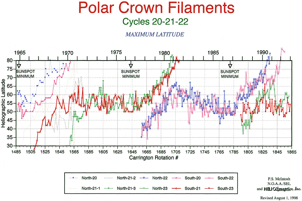
Figure 2. Maximum, poleward-most latitudes of filaments in the primary and secondary PCFs for both hemispheres for cycles 20–22. Both hemispheres have been folded together. P. McIntosh produced this figure in 1998; also see Figure 4 in Webb (1998) and Figure 5 in McIntosh (2003).

Time-series stack-plots of zones of the maps help to identify and track large-scale solar features. These include active longitudes, CHs and polarity boundaries over SC time scales (e.g., McIntosh, 2003; Gibson et al., 2017). Figure 3A shows a black and white figure P. McIntosh used to display the large-scale polarity patterns for high solar latitudes for 1964–1967 comparing the north (left) and south (right) poleward zones. The barber-pole patterns denote the varying rotation rates of the long-lived, large-scale patterns. These show how the polarities reverse during the SC and the difference in rotation rates between the poleward and equatorial zones. Decadal-long stack plots have established the evolution of polar crown gaps, polarity reversals and longitudinal drifts in patterns that circle the Sun over a cycle (McIntosh and Wilson, 1985; McIntosh et al., 1991; McIntosh, 2003). Analysis of these patterns led to development of a model of emerging flux and surface evolution (McIntosh and Wilson, 1985; Wilson and McIntosh, 1991).

FIGURE 3

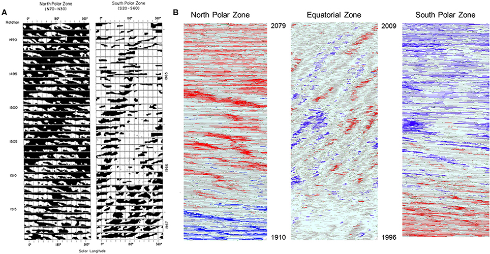
Figure 3. (A) Figure by P. McIntosh displaying the large-scale polarity patterns for high solar latitudes for 1964–1967 comparing north and south poleward zones for each 360° CR. The barber-pole patterns denote the varying rotation rates of the patterns. (B) The same stack-plotting, but for the entire McA SC 23 (13 years) data in 40° zones: North polar zone = N30–N70°, Equatorial zone = S20–N20°, South polar zone = S30–S70°.

McIntosh's maps have been used, more recently, to study the morphology and evolution of coronal cavities, as magnetic coronal mass ejection precursors (Gibson et al., 2010), and to study solar activity during the last prolonged minimum (Thompson et al., 2011; Webb et al., 2011). As we have progressed in archiving and digitizing the McIntosh archive, we have made it available online as described below. Already groups around the world have started to use it in scientific analyses, e.g., Gibson et al. (2017); Mazumder et al. (submitted).

Data Format and Processing Details

Summary of Method²

Our original goal of preserving the original data and organizing it by scanning and digitally processing the maps into consistent, machine-readable format has been achieved with the help of NSF support. As a result we have created what we call the McIntosh Archive (McA). We hope that the McA will be utilized by scientists and the public for many years. This program has been accomplished with a team from Boston College/Institute for Scientific Research (ISR) in Newton, MA and the NCAR/High Altitude Observatory (HAO) in Boulder, CO. A description and access to the archive can be found at: https://www2.hao.ucar.edu/mcintosh-archive/four-cycles-solar-synoptic-maps.

Our process is summarized next. The maps are preserved in three formats: (1) Level 0 GIF images which are direct scans of the original hand-drawn McIntosh maps; (2) Level 1 GIF images which have been cropped, reoriented and scaled for consistency; (3) Level 3 FITS format files and associated GIF images characterize the fully processed maps. The original maps are scanned and saved as Level 0 GIFs in the Archive. These are then read by an IDL routine (levelone.pro) which digitizes them in a consistent and reproducible manner. In particular, the code: (1) identifies the Carrington latitude/longitude boundaries of the scanned map, crops the space outside these boundaries, and rotates to ensure the maps have the same orientation; (2) resizes so that all maps have the same resolution; and (3) identifies latitude and longitude coordinates for each pixel. The maps are then saved as the Level 1 GIF images in the archive, with metadata relating Level 0 to Level 1 preserved in intermediate data files, ultimately to become part of the Level 3 FITS files (see below).

The Level 1 GIFs are read into Photoshop and the filaments, filament channels, coronal holes (if present), sunspots, and plage are traced over with colors unique to each type of feature. This represents the primary human intervention to the process, and is a straightforward matter of identifying large dots as sunspots and plage areas, thick lines as filaments, hatched lines as CH boundaries, etc. A second IDL code (leveltwo.pro) then reads the gif output of the Photoshop processing, replacing all pixels that do not possess the specific feature colors with white pixels, and thus removes no-longer-needed information such as text and the original overplotted latitude-longitude grid. Five points of this initial grid are preserved (marked with an identifying color during the Photoshop session) as a means of quantifying any error potentially arising from a non-rectangular grid (these errors are very small). A second Photoshop session then fills in CHs and quiet sun with colors defining their polarity. Since the initial session created continuous boundaries, this is a straightforward and reproducible step achieved simply by selecting the spaces within the boundaries and choosing a color based on the + and – symbols on the original maps.

The final IDL code (levelthree.pro) combines the metadata saved during the previous IDL steps of the digitization process with metadata entered into the spread-sheet record of the archive, which includes information such as data sources and cartographers for each map. The map data are now basically in the form of a uniform grid of numbers, each of which can be translated to a color that uniquely identifies the associated solar feature type. Further analysis is done as part of this code that examines quiet sun pixels surrounding sunspots and plage in order to associate a signed polarity with them, resulting in further refinement of color/feature diversity. The map data, longitude-latitude data, a grid of polarity assigned to each pixel, and all metadata are then save as the Level 3 FITS files for the archive.

Finally, the IDL code calls a subroutine (plotfinal.pro) which creates standardized Level 3 GIF images from the FITS files for a given CR number (e.g., Figure 1, bottom). This code can also be used to create customized GIFs from the FITS files if so desired. For a given CR, plotfinal.pro can produce up to 16 permutations of the (FITS) mapping variables that are output as “final” GIF files depending upon keyword settings. These are 8 with a heliographic grid and annotations and 8 with no grid and annotations. Other combinations include extensions of +/−30° for −30° to 390° in solar longitude, or only 0°-360° in solar longitude; missing yellow data poleward of +/−70° in solar latitude, or missing yellow with only CH boundaries, or CHs filled in with missing yellow negative or positive polarity, or all colors filled in near the poles. The final file names reflect these combinations. Since all the final CR maps have the same color system and known scaling, features can be intercompared over many CRs, with time and as a function of solar cycle. We are also writing other codes to permit efficient searches of the map arrays.

A key feature of the final Level 3 maps is the PILs which bound opposite-polarity photospheric magnetic fields. Solar features included on the maps include CHs having positive-polarity magnetic field and their boundaries, positive magnetic fields, CHs having negative-polarity magnetic field and their boundaries, negative magnetic fields, PILs, filaments, sunspots, and plage groups. These features are identified on the final archive maps using 10 IDL colors (numbers) that allow digital sorting and searches for data analysis. In addition, missing data on a map are marked in yellow, usually near the poles above 70°.

The plotfinal.pro code along with the processed maps is archived at the NOAA's National Centers for Environmental Information (NCEI) in their final, searchable form at: https://www.ngdc.noaa.gov/stp/space-weather/solar-data/solar-imagery/composites/synoptic-maps/mc-intosh/. The archive is publicly available and also accessible through the above HAO online site.

Also, we have included comprehensive metadata in the Level 3 FITS files that incorporate all the information needed to describe the original, Level 0 form of the maps. A separate metadata spreadsheet, containing information on data sources and cartographic notes, is maintained for all of the processed maps and is also available through the online sites. For each CR map the spreadsheet contains information about the McA data sources, the individual(s) responsible for map creation, and comments. The data types include filaments and other tracers of PILs, photospheric magnetic field polarities, CH boundaries, sunspots and plage. The data sources vary with time and include ground-based telescopes at various solar observatories, including NOAA-Boulder, Big Bear Solar Observatory (BBSO), Meudon, National Solar Observatory (NSO), He-I 10,830 Å (NSO), SOON and ISOON, Mauna Loa Solar Observatory (MLSO), GONG, He-I SOLIS, He-II 304 Å and MDI images on the SOHO spacecraft, etc.

Current Status of the MCA

When completed the McA CR maps will permit measurements of the evolution of the large-scale, global magnetic field of the Sun over the course of four solar cycles. However, there are incomplete or missing maps during this period that need to be completed using original data sources. The archive for SC 23, from 1996 into 2009, is complete (e.g., Gibson et al., 2017), as is the entire period between the maxima of SCs 21 and 22. The scanning of all of the original maps, 1964–2009, to Level 1 has been completed. As of this writing we have brought all the original maps that we consider were completed to the final Level 3. Presently 3/4 of the 600 possible CR maps have been completed to Level 3, starting in 1966 in SC 20 to 2009, the start of SC 24, but with gaps in SCs 20, 21, and 22. Here we are presenting scientific results based on a complete processing of all the original maps that we consider final.

Future Processing Work

Our processing goal is to complete the incomplete or missing maps so that the McA will provide a continuous record of solar surface structures over four SCs for the community. The remaining processing tasks include completing about 100 incomplete maps from the original archive and creating 26 missing maps. As part of this processing, we are adding CHs to the maps when sufficient CH observations are available. Most of these CHs are from Kitt Peak Solar Observatory He-I 10,830 Å observations when these images became available in April 1974 with CR 1614. To date we have added He-I 10,830 Å CHs to most of the otherwise complete maps between 1974 and 1981. In addition, we added CHs for 8 of the 10 CR maps from CR1601-1610 (in 1973 and early 1974) during the manned portions of the Skylab mission using the EUV He 304Å observations from Bohlin and Rubenstein (1975) and reproduced for CR1605 and CR1609 in Bohlin and Bohlin and Hulburt (1977).

In addition, we have scanned and will process into the McA the atlas of 132 Hα synoptic charts for SC 19 that was produced by Makarov and Sivaraman (1986). This will provide 5 full SCs of CR maps that are in the same consistent, machine-readable format for analyses of filaments and polarity boundaries. We note that no consistent CH boundary data are available before the Skylab period in 1973.

Analysis Highlights

Solar-Cycle Evolution of Closed and Open Magnetic Structures

A unique characteristic of the McIntosh archive maps is that they can simultaneously represent both closed and open magnetic structures over a variety of time scales. Figure 4 shows the global evolution of sunspots, plage and filaments for all of the McA data processed to date starting with CR 1513 in October 1966 and ending with CR 2086 in July 2009 in heliolatitude vs. time. Sunspots and plage are plotted together in Figure 4A and reveal the classic butterfly diagram, with sunspots appearing at solar minimum, first at high latitudes then emerging progressively closer to the equator during the cycle progression.

FIGURE 4

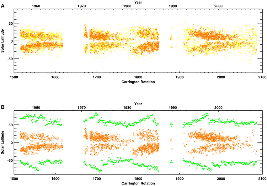
Figure 4. Butterfly-type plots of all of the McA data processed to date starting with CR 1513 in October 1966 and ending with CR 2086 in July 2009. The Year scale is at the top and the CR scale at the bottom. (A) McA plot of sunspots (orange) and plage (yellow), both associated with ARs and revealing the classic butterfly pattern. On each map the sunspot color denotes the sizes and locations of sunspots visible on H-alpha images, whereas the plage color roughly corresponds to the area of bright plage on Hα images. (B) Plot of the McA sunspots (orange) and the poleward-most filament boundaries per CR (green) for this period. The same “rush to the poles” as shown in Figure 2 during the rise phases of both SC 22 and 23 is evident as well as the appearance of the new PCF after each maximum.

In Figure 4B the sunspots in orange and the location of the most poleward filament for each CR in green dots are plotted together. The polemost filaments indicate the “rush-to-the-poles” which traces the solar magnetic polarity reversal process (e.g., Altrock, 1997). After the polarity reversal in each hemisphere, the old polar crown filament is replaced by a secondary filament band (McIntosh, 1992). This process has been traced back to SC 14 in 1904 using filament data from Meudon Observatory (Makarov and Sivaraman, 1983, 1989; Li et al., 2008) and from Meudon and Kislovodsk Observatories (Tlatov et al., 2016), and recently back to SC 15 in 1919 from newly processed KSO Hα data (Chatterjee et al., 2017). This behavior is also mimicked in green line coronal observations extending back to 1939 (Minarovjech et al., 1998).

Figure 5A is a plot of the maximum latitude per CR for PCFs from the original McIntosh maps, including the “secondary” PCF that appears at lower latitudes and replaces the “true” PCF after the solar field reverses. It is in the same format as Figure 2. Pat McIntosh (McIntosh, 2003) produced this expanded plot by combining the “rush-to-the-poles” period of SC 22 (Figure 2) with then-new data from SC 23. Our version of this plot from the newly processed, digitized McA is shown in Figure 5B, in the same coordinate system with the north and south polemost filaments superimposed with different symbols (note we do not show the secondary PCF in this plot). We can see that it is a good match to McIntosh's older plot. Mazumder et al. (submitted) are also using the McA data set to plot filament, PIL, and CH parameters. They find that over SCs 21–23 filament and PIL lengths are well correlated with the sunspot cycle.

FIGURE 5

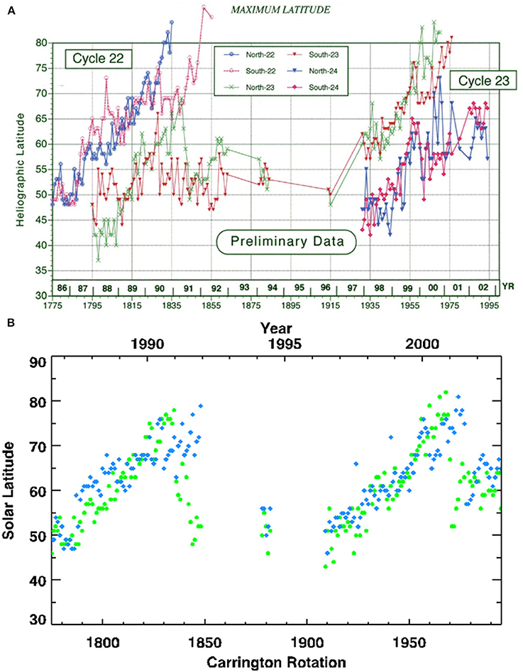
Figure 5. (A) Plot of the maximum latitude per CR for PCFs from original McIntosh maps, including the “secondary” PCF that appears at lower latitudes and replaces the “true” PCF after the solar field reverses. Like the SC 20-22 plot in Figure 2, P. McIntosh produced this expanded plot in 2003 (Figure 6 in McIntosh, 2003) comparing the “rush-to-the-poles” periods of SC 22 and 23. (B) The current version of this plot for the McA that has been completed to date for SCs 22 and 23. This plots only the single polemost filament location from each CR map, and so does not separate the true and secondary PCF branches as the top plot does. For each SC the northern hemisphere locations are plotted as filled green circles and the southern as filled blue diamonds.

McIntosh (e.g., 2003) first noted that both the polar crown of filaments and sunspots begin around the same period early in a cycle around 40° latitude. Then they diverge with the PCF moving poleward and sunspots and active regions moving equatorward. He also plotted the secondary polar crown which also moves poleward separated by at least 15° from the primary crown. This suggests that two large cells of opposite polarity in each hemisphere move poleward, a complication for the Babcock-Leighton model that features transport of active region-sunspot flux. He noted that the poleward motions of these four polar crowns were very similar for SCs 21–23, suggesting evidence of deeper-seated dynamo activity. Finally we note that when the primary crown reaches the poles and disappears, the secondary crown stops its motion, around latitude 55°, before either remaining at that latitude or drifting slightly equatorward through the remainder of the cycle. During the rise of the next cycle it then begins its rush to the poles as the primary crown of that cycle.

Figure 6A is a plot of the locations of the pole-most CH boundaries for each CR during SC 23. The closed (open) circles denote the most northward (southward) extensions of the CH boundaries on each CR. These plots highlight the diverging behavior of what appear to be two populations of CHs: the polar CHs that move poleward and low-latitude CHs that track the sunspot butterfly pattern. Figure 6B shows this same plot with the zonal flows (torsional oscillations) of the near-surface magnetic field overlaid. The zonal flows use GONG observations from 1995 to the present (Howe, 2016). This overlay demonstrates that the CH locations match well with the poleward and equatorward zonal flows over SC 23.

FIGURE 6

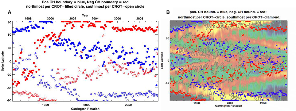
Figure 6. (A) The poleward-most CH boundaries per CR for SC 23. Closed (open) circles indicate the most northward (southward) extensions of CH boundaries for each CR. Red and blue indicate magnetic polarity. (B) This same plot overlaid on a plot of the zonal flows (torsional oscillations) of the near-surface (0.99 R_⊙) magnetic field from GONG, MDI, and HMI data, covering the period from the beginning of the GONG observations in 1995 to the present (from Howe, 2016; prepared by R. Komm).

Recent analyses of small-scale magnetic features, such as EUV bright points, magnetic regions of influence, g-nodes, torsional oscillations, sunspots and CH centers (e.g., McIntosh et al., 2014; Bilenko and Tavastsherna, 2016; Fujiki et al., 2016), indicate that the activity bands of these features emerge at about 55° north and south latitudes and reach the equator in 18–19 years. This is again evidence that solar cycles are extended (e.g., Cliver, 2014). This important 55° latitude zone is also evident in the McA map patterns of polar and low-latitude CHs with opposite polarities separated by the PCFs. Earlier, Webb et al. (1984) and Harvey and Recely (2002) emphasized this development of polar CHs reforming as a consequence of the motion of low-latitude UMRs and CHs poleward. The divergence patterns of the PCF, sunspot zones, CHs and small-scale features and their tendency to follow the poleward and equatorward slopes of the wedge-shaped torsional oscillation bands are very important for understanding internal dynamo processes. Determining the slopes, how well the different feature slopes match, and whether the patterns repeat in other SCs is for future work.

Figure 7 combines the sunspot, filament and CH locations for the entire McA data processed to date, showing how the patterns discussed for SC 23 are repeated in earlier cycles. In addition, the plot illustrates how the positive and negative-polarity open magnetic fields surround the closed-field filaments and sunspots globally. For the period for which we have processed CH data, from just before the maximum of SC 21 (1980) to the start of SC 24 (2009), this demonstrates well how the dual cells of opposite-polarity in the higher latitudes of each hemisphere track each other through each SC, and how consistent the offset is between the higher-latitude open and closed regions and the lower latitude closed regions (sunspots and plage). These large-scale rearrangements of the open flux in unipolar areas and the formation of the polar CHs in SC 23 and 24 have recently been studied by Golbeva and Mordvinov (2017). These large-scale motions are somehow tied to the internal fluid dynamics of the Sun, and must be accounted for in dynamo models.

FIGURE 7

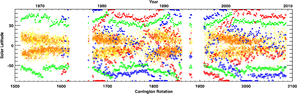
Figure 7. Butterfly-type plot of all of the McA data processed to date starting with CR 1513 in October 1966 and ending with CR 2086 in July 2009. The Year scale is at the top and the CR scale at the bottom. This plots for each CR all sunspots (orange), the poleward-most filament boundaries (green), and the poleward-most CH boundaries (red and blue). As in Figure 6A, closed (open) circles indicate the most northward (southward) extensions of CH boundaries for each CR, and red and blue indicate magnetic polarity.

Mazumder et al. (submitted) have recently studied the time variation of CH areas calculated from the McA maps. They find that the total CH area on the Sun is dominated by high latitude (>40° latitude) CHs during most of a SC. As is well known, the total CH area is anticorrelated with sunspot number, sharply dipping to a minimum at SC maximum. These minima were reached in 1990–1991 in SC 22 and 2001 in SC 23. They also find a north-south asymmetry in the CH areas around these same times, which is indicative of a lag or temporal offset in the magnetic field development between hemispheres during these SCs (see next section The Polar Field Reversal Process).

The Polar Field Reversal Process

Of particular interest with our currently available processed data is the evolution of the polar magnetic regions of the Sun and how the rush to the poles and other patterns occur during the period when the polar fields reverse near each SC maximum. We see in Figure 7 that there is data coverage during these epochs for three consecutive SCs. In the north these occur in SC 21 around CR 1700, SC 22 ~ CR 1830, and SC 23 ~ CR 1970. In the south the reversals lag those in the north, in agreement with the early dominance of magnetic flux and its reversal in the northern hemisphere during each of the last 4 SCs (e.g., Petrie, 2015). This process in the south during SC 22 is obscured here because of the long data gap between the maximum of SC 22 and the start of SC 23. The polar field reversal process is evident in these data by two features: (1) the end of the filament rush to the poles, i.e., the polemost filament boundary decreases suddenly as the PCF disappears and the secondary crown is recorded as “polemost” (see Figure 5), and (2) the polar CH disappears before this and, sometime later, the polarity of the polemost CH reverses. This is revealed at the north pole as blue-to-red, red-to-blue and blue-to-red CH color changes during the three cycles, with the opposite pattern in the south.

Because the processed data set is in a consistent, machine-readable format, the maps can be displayed in various ways. One method that we find especially useful for displaying the polar reversal process is by displaying the Level 3 data (which is in latitude-longitude coordinates for each CR) mapped onto a sphere that can be viewed from different vantage points. This is illustrated for one CR in Figure 8 which shows the north and south polar views for CR 1728 plus two side-on views 180° apart centered on the equator. The online movies associated with Figure 8 (Movies 3–6) show the polar reversals and also the common occurrence of spiral patterns evident in the coronal holes/polar crown filaments. This type of pattern has been noted in coronal cavities (Karna et al., 2017) and in helioseismic ring-diagram analyses of near-surface flow anomalies (Bogart et al., 2015).

FIGURE 8

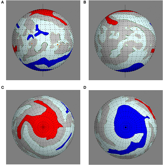
Figure 8. An example of the transformation of the Mercator-type rectangular McA synoptic maps into a spherical coordinate system. In this coordinate system, the data for each CR appears on a rotating sphere and can be viewed from different vantage points. This is illustrated for one CR (1728) showing the two side-on views 180° apart centered on the equator and at (A) 45° and (B) 225° Carrington longitudes plus (C) north and (D) south polar views, respectively. Movies 3-6 of these same four views for the final, Level 3 McA data set are provided in the Supplemental Material.

The polar magnetic field reversal process was first studied in some detail for SCs 20 and 21 by Webb et al. (1984). The goal was to use the then-newly understood CH boundary mapping to better constrain dynamo models. CH data were obtained from X-ray rocket and OSO-6 images and HAO K-coronameter white light maps for SC 20 and He-I 10,830 Å maps for SC 21. These data were combined with McIntosh's original synoptic maps to determine the timing of five events around the maximum of each SC in each hemisphere: the sunspot number peak, the polarity reversal, the disappearance of the PCF, the first appearance of mid-latitude CHs of new-cycle polarity, and the earliest complete coverage of each pole by a coronal hole. The time offsets, or lags between the reversal and the last three events was also determined. As discussed above, with the processed McA we can now extend this type of study over four consecutive SCs through SC 23.

Studies of Active Longitudes

As discussed in section Previous Studies Using the Original McIntosh Maps time-series zonal stack plots of the synoptic maps are valuable for tracking over SC time scales large-scale features, such as CHs, active longitudes and polarity boundaries. Active longitudes, where sunspots and magnetic flux preferentially emerge (e.g., de Toma et al., 2000), are easily tracked on stack plots (McIntosh, 2003). The persistence of two active longitudes 180° apart over 100 years has been found in sunspot records (e.g., Berdyugina and Usoskin, 2003), as well as in recently digitized white-light images from KSO (Mandal et al., 2016b).

Webb et al. (1978) used the McIntosh maps to link the evolution of CH boundaries with filament eruptions and coronal transients. The evolution of so-called “switchback” neutral lines, relatively sharp reversals in the direction of a PIL, are common features of large-scale PILs and may indicate stress buildup leading to increased solar activity and possibly eruptions (e.g., van Ballegooijen et al., 1998). Their evolution can easily be tracked on McA maps (e.g., McAllister et al., 1996).

Decade-long stack plots have established the evolution of polar crown gaps, polarity reversals and other longitudinal pattern drifts that circle the Sun over a cycle. McIntosh et al. (1991) contains an atlas of stack plots of the Hα maps over two full SCs, from 1966 to 1987. The long-term zonal stack plots show clearly the evolution of magnetic structures over narrow latitude bands. Latitude bands covering ~10 to tens of degrees in each hemisphere or centered at the equator are selected from each map, and plotted or “stacked” one above the other in time series. The time series are made adjustable from a few consecutive maps to maps covering a solar cycle or so in time. We show in Figure 3A an original figure P. McIntosh produced to display the large-scale polarity patterns for high solar latitudes for 1964–1967. We have written code based on the McIntosh et al. (1991) work to produce similar stack plots from the digitized McA. The three sets in Figure 3B illustrate this stack-plotting, but for the entire colorized McA SC 23 (13 years) data in 40° zones for the northern, equatorial, and southern zones. These patterns are associated with, e.g., active longitudes of magnetic flux emergence (de Toma et al., 2000), recurring high-speed solar wind streams (Gibson et al., 2009), and periodic forcings of geospace and the upper atmosphere (Emery et al., 2009, 2011). The McA stack plots demonstrate clear periodicities in both closed (e.g., sunspot) and open (e.g., CHs) fields, magnetic polarity reversal during the SC, and differential rotation rates between the poleward and equatorial zones.

Figure 9 is a sequence of equatorial slices (−20° to +20° heliolatitude) stacked along a curving, snake-like axis advancing in time using the McA data for all of SC 23 (CRs 1910–2084) as in Figure 3. The width of the “snake” is the 360° heliolongitude for each CR (after, e.g., McIntosh and Wilson, 1985). The colors follow the key as in Figure 1 (bottom). Active longitudes are evident in quiet sun, sunspots, and coronal holes. A ~180° longitudinal asymmetry is particularly evident just after solar maximum; this is consistent with studies spanning ~100 years of sunspot active longitudes (e.g., Berdyugina and Usoskin, 2003).

FIGURE 9

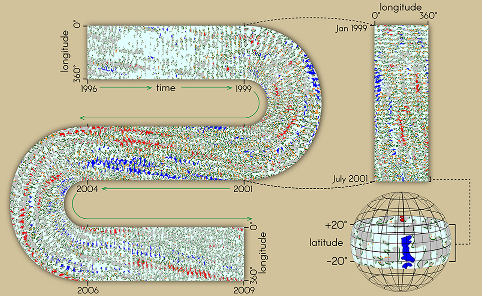
Figure 9. A sequence of equatorial slices (−20° to +20° latitude) is stacked along a curving axis, like a snake, advancing in time through CRs 1910-2084 (SC 23); width is longitude (after, e.g., McIntosh and Wilson, 1985). Colors are as in Figure 1 (bottom). The panels on the right show how an equatorial latitude strip from one CR is patched into a stackplot which in turn becomes a curvilinear part of the entire “snake” that traverses all of SC 23.

Linking Large-Scale Patterns to the Solar Wind

Persistent, rotating, low-latitude CHs drive periodic behavior, both in the solar wind and in the Earth's environment. This was studied at length during the decline of SC 23 and the following extended solar minimum (e.g., Temmer et al., 2007; Gibson et al., 2009; Luhmann et al., 2009). This period included the Whole Heliosphere Intervals in 2008–2009 (e.g., Gibson et al., 2011; Thompson et al., 2011; Webb et al., 2011). This otherwise quiet time period, e g., with few sunspots, was characterized by sustained longitudinal structure, with three and then two near-equatorial open-field regions, as shown in the top part of Figure 3B, middle panel.

Figure 10 compares CR stackplots showing (left) in-ecliptic solar wind speeds, from NASA OMNI data, and (right) surface features from the McA during SC 23. The solar wind speeds versus Carrington longitude plot reveals the presence of high-speed streams that recur over multiple rotations and fade in and out over time (see also Lee et al., 2011). The occurrences of these streams line up well with the presence of large equatorial CHs as recorded in the McA maps (Cranmer et al., 2017; Gibson et al., 2017). The long-lived coronal holes (blue/red) in panel (b) rotate at a rate somewhat faster than the 27.275 day Carrington rotation, and thus have a positive slope in this plot. This correlates well with the slopes seen in the fast wind streams indicated in panel (a).

FIGURE 10

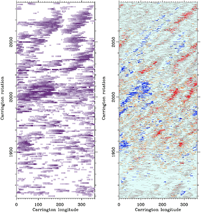
Figure 10. CR stackplots showing (left) in-ecliptic OMNI wind speeds and (right) surface features from the McA, both for the duration of SC 23. In the left panel, white denotes v ≤ 450 k ms⁻¹ and increasingly darker shades of purple eventually saturate at the darkest color for v ≥750 k ms⁻¹. Longitudes have been offset by 50.55°, or 3.83 days, to account for propagation from the Sun to 1 AU at a mean speed of 450 k ms⁻¹. The right panel shows equatorial (±20° from equator) features, with blue [red] showing coronal holes of positive [negative] polarity, cyan [gray] showing quiet regions with predominantly positive [negative] polarity, orange indicating sunspots, and green indicating filaments; from Cranmer et al. (2017).

The patterns shown in Figure 10 extend to the Earth's space environment and upper atmosphere. Correlations are found between high-speed solar wind streams and modulations of the aurora and geomagnetic indices, radiation belts, ionosphere, and thermosphere (Gibson et al., 2009; Solomon et al., 2010; Lei et al., 2011). Long-time series analyses over years and decades show periodicities in all of these quantities that may be associated with periodicities in the fast solar wind, and consequently the distribution of open magnetic flux at the Sun in the form of CHs (Emery et al., 2011).

Studies of Differential Rotation

Figures 3B, 9 clearly show that the equatorial CHs between +/– 20° solar latitudes shift eastward with time, completing a full circle in about 180 maps, or 2.5 years. A Carrington rotation is 27.38 days relative to our observing position on the Earth (the sidereal rate), where the equatorial zone rotates faster than mid-latitudes or the poles. Thus, the observed eastward shift of low-latitude coronal holes embedded in polarity regions could simply represent the lower latitudes rotating at about 25 days, provided CHs are fixed with respect to the solar surface. However, the apparent rotation eastward is not as strong during the solar minimum periods at the top and bottom of the plots when there are fewer low-latitude CHs, which may indicate a differential rotation of the CHs that departs from solar surface flow rates.

Figure 3B shows for SC 23 the equatorial zone and the northern and southern polar zones. The polar zones near solar minimum (at the top and bottom of the plots) exhibit unipolar CHs at all latitudes, but at solar maximum and in the declining phase the slower polar rotation rate is manifest. The CHs in the polar zones show a westward drift at solar maximum, which is much more pronounced in the northern hemisphere with both the blue positive polarities in 1996, and the red negative polarities in 2002 compared to the southern hemisphere. Again, this reflects a variation in differential rotation rates in the CH vs. solar surface flows. It is of interest to see whether or how these interhemispheric differences appear in earlier solar cycles.

The differential rotation rate in active longitudes tends to match the surface flow at that latitude (e.g., Usoskin et al., 2005; Mandal et al., 2016b). This contrasts with individual sunspots that rotate faster than the surface flow, suggesting that they are rooted below the near-surface shear layer (Thompson et al., 2003). Polar CHs can show rigid rotation, while CHs at low latitudes rotate differentially but also have a variability that might be due to the lifetimes of CHs and the phase of the SC (e.g., Ikhsanov and Ivanov, 1999). This variability may contribute to the range in the CH slopes observed in the figures, these patterns and their slopes can be readily measured on the MCA maps.

Conclusion

Summary

We have demonstrated some examples of how the newly-processed McIntosh Archive (McA) maps can be used to investigate the long-term variability of solar surface features. Our work highlights understanding the sources and evolution of active regions, CHs, filaments and PILs, how the rotation rates of these features vary over SCs, and the long-term variation of the toroidal and poloidal components of the magnetic field and their connection to the internal dynamo. Thus, the McA maps promote studies of the SC variation of both closed and open magnetic structures in a new approach, and eventually will cover five contiguous SCs: 19–23.

Discussion

A unique aspect of the McIntosh archive is its capability to simultaneously display closed and open magnetic structures over a range of time scales. Completing the fully McA digitized maps will offer the community a comprehensive resource to address some key questions such as: Where are closed and open magnetic features embedded? How do these locations depend on feature lifetime, SC phase and latitude? How is the evolution of closed and open magnetic features associated with surface flows over SC periods? How do active longitudes for both closed and open magnetic features vary over SCs? The answers to these questions are important for our understanding of the solar dynamo and of periodic variations in Earth's environment.

Over past decades the capabilities of dynamo-type models have increased to today's fully 3-D MHD numerical simulations, with the goal of being able to reproduce the solar cycle in terms of surface manifestations such as sunspots and the other patterns evidenced in the McA maps (e.g., Charbonneau, 2010). However, we still lack sufficient knowledge of the solar interior, especially the deep convection zone. Recently, some research has focused on the SC-variation of small-scale magnetic features such as EUV bright points and their relation to torsional oscillations and “giant cells” as indicators of magnetic activity in the deeper-seated convection zone (e.g., McIntosh et al., 2014; McIntosh et al., under review). The subsurface flow anomalies noted in section The Polar Field Reversal Process could be related to east or westward surface motions of extended convective structures “wound up” by differential rotation (e.g., Hathaway et al., 2013). Studies of the motions of such patterns compared to subsurface differential rotation profiles and other helioseismic data can address whether or not they are surface manifestations of deep convective cells (Bogart et al., 2015). Also, zonal flow anomalies at high latitudes could be related to the evolution of the torsional oscillation at high latitudes and, therefore, the evolution of the solar cycle (discussed in section Solar-Cycle Evolution of Closed and Open Magnetic Structures and shown in Figure 6). The McA will be very useful for all these studies for understanding the surface features and transport processes in the context of new models and simulations.

The McA can also be a very useful tool for improving our understanding of and ability to predict solar activity and space weather. Such predictions are needed to protect assets vital to our national security and the operations of technologies used worldwide in civilian daily life. Analyses of this accurate baseline of solar activity that covers ~45 years (four consecutive SCs) can enhance our understanding of solar activity and our capability to predict it. In addition, improving public access to historic measurements of CHs and filaments is helping researchers to better understand and study the connection between these phenomena at the Sun and their effects at Earth (e.g., Knipp et al., 2016).

Future Work

When the McA is completed, we plan to analyze the full data set and publish the results. Some of the topics we are working on include: (1) Analysis of the rush to the poles phenomenon involving the PCFs, CHs, and unipolar regions; (2) Analysis of the divergent slopes of the PCF, sunspot zones, CHs and small-scale features over many SCs and what they tell us about internal dynamo processes; (3) Extending the results of the Webb et al. (1984) study on the polar field reversal process through SC 23; (4) Analysis of the differential rotation differences, such as for CHs, using time-variation analyses programs as a function of solar latitude, solar cycle, and hemisphere; (5) Studies of active longitudes and switchback PILs as related to solar activity, eruptions and space weather; (6) Analysis of linkages between large-scale solar surface patterns and solar wind streams and the terrestrial environment.

Author Contributions

DW is PI of this work and wrote most of the paper. IH and RM performed the image scanning, cartography and digitization for the project. BE supervised the work of IH and RM at HAO and contributed to analysis of the surface feature motions. SG wrote the initial scanning and plotting software for the project, produced the FITS files, and contributed to the analyses. AM wrote the software for the spherical map projections. TK assisted the PI at BC, managing the image and metadata data at BC, IDL manipulation of the data files and plotting, and managing the images FITS files.

Conflict of Interest Statement

The authors declare that the research was conducted in the absence of any commercial or financial relationships that could be construed as a potential conflict of interest.

Acknowledgements

We dedicate this project to Patrick McIntosh who passed away in October 2016. We are thankful to his daughter, Beth Schmidt for granting permission to use his original data. We consider Pat to be a founding Father of what we now call Space Weather, because of his innovative work in forecasting research starting at the Space Environment Laboratory at the National Oceanic and Atmospheric Administration (NOAA) in Boulder. The authors were supported by NSF RAPID grant 1540544 and NSF grant 1722727. The National Center for Atmospheric Research (NCAR) is supported by the National Science Foundation. The repository for the data discussed here is available at: https://www.ngdc.noaa.gov/stp/space-weather/solar-data/solar-imagery/composites/synoptic-maps/mc-intosh/, and at: https://www2.hao.ucar.edu/mcintosh-archive/four-cycles-solar-synoptic-maps.

Supplementary Material

The Supplementary Material for this article can be found online at: https://doi.org/10.6084/m9.figshare.6837641

Movie 1. Original L1 CR maps.

Movie 2. Final processed L3 CR maps.

Movie 3. Spherical coordinates movie centered on Heliolongitude of 45°.

Movie 4. Spherical coordinates movie centered on Heliolongitude of 225°.

Movie 5. Spherical coordinates movie of Solar North pole.

Movie 6. Spherical coordinates movie of Solar South pole.

Footnotes

1. ^This history is also discussed in Webb et al. (2017).

2. ^Our method is also discussed in Webb et al. (2017).

References

Altrock, R. C. (1997). An ‘extended solar cycle' as observed in FeXIV. Sol. Phys. 170:411. doi: 10.1023/A:1004958900477

CrossRef Full Text | Google Scholar

Babcock, H. W. (1961). The topology of the sun's magnetic field and the 22-year cycle. Astrophys. J. 133:572. doi: 10.1086/147060

CrossRef Full Text | Google Scholar

Berdyugina, S. V., and Usoskin, I. G. (2003). Active longitudes in sunspot activity: century scale persistence. Astron. Astrophys. 405:1121. doi: 10.1051/0004-6361:20030748

CrossRef Full Text | Google Scholar

Bilenko, I. A., and Tavastsherna, K. S (2016). Coronal hole and solar global magnetic field evolution in 1976 – 2012. Sol. Phys. 291, 2329–2352. doi: 10.1007/s11207-016-0966-2

CrossRef Full Text | Google Scholar

Bogart, R. S., Baldner, C., and Basu, S. (2015). Evolution of near-surface flows inferred from high-resolution ring-diagram analysis. Astrophys. J. 807:125. doi: 10.1088/0004-637X/807/2/125

CrossRef Full Text | Google Scholar

Bohlin, J. D., and Hulburt, E. O (1977). “An observational definition of coronal holes, Chapter 2,” in Coronal Holes and High Speed Wind Streams, ed B. Jack Zirker, A Monograph from Skylab Solar Workshop I (Boulder, CO: Colorado Associated University Press), 27.

Bohlin, J. D., and Rubenstein, D. M. (1975). Synoptic Maps of Solar Coronal Hole Boundaries Derived From He 304A Spectroheliograms From the Manned Skylab Missions. Report UAG-51, World Data Center A for Solar-Terrestrial physics, NOAA.

Charbonneau, P. (2010). Dynamo models of the solar cycle. Living Rev. Sol. Phys. 7:3. doi: 10.12942/lrsp-2010-3

CrossRef Full Text | Google Scholar

Chatterjee, S., Banerjee, D., and Ravindra, B. (2016). A butterfly diagram and Carrington maps for century-long Ca ii k spectroheliograms from the Kodaikanal Observatory. Astrophys. J. 827:87. doi: 10.3847/0004-637X/827/1/87

CrossRef Full Text | Google Scholar

Chatterjee, S., Hegde, M., Banerjee, D., and Ravindra, B. (2017). Long term study of the solar filaments from the synoptic maps as derived from H? spectroheliograms of Kodaikanal Observatory. Astrophys. J. 849:44. doi: 10.3847/1538-4357/aa8ad9

CrossRef Full Text | Google Scholar

Cliver, E. W. (2014). The extended cycle of solar activity and the Sun's 22-year magnetic cycle. Space Sci. Rev. 186, 169–189. doi: 10.1007/s11214-014-0093-z

CrossRef Full Text | Google Scholar

Cranmer, S. R., Gibson, S. E., and Riley, P. (2017). Origins of the ambient solar wind: implications for space weather. Space Sci. Rev. 212:1345. doi: 10.1007/s11214-017-0416-y

CrossRef Full Text | Google Scholar

de Toma, G., White, O. R., and Harvey, K. L. (2000). A picture of solar minimum and the onset of solar cycle 23. I. global magnetic field evolution. Astrophys. J. 529:1101. doi: 10.1086/308299

CrossRef Full Text | Google Scholar

Emery, B. A., Richardson, I. G., Evans, D S., and Rich, F. J. (2009). Solar wind structure sources and periodicities of auroral electron power over three solar cycles. J. Atmos. Solar Terr. Phys. 71, 1157–1175. doi: 10.1016/j.jastp.2008.08.005

CrossRef Full Text | Google Scholar

Emery, B. A., Richardson, I. G., Evans, D. S., Rich, F. J., and Wilson, G. R. (2011). Solar rotational periodicities and the semiannual variation in the solar wind, radiation belt, and aurora. Sol. Phys. 274, 399–425. doi: 10.1007/s11207-011-9758-x

CrossRef Full Text | Google Scholar

Fox, P., McIntosh, P., and Wilson, P. R. (1998). Coronal holes and the polar field reversals. Sol. Phys. 177:375. doi: 10.1023/A:1004939014025

CrossRef Full Text | Google Scholar

Fujiki, K., Tokumaru, M., Hayashi, K., Satonaka, D., and Hakamada, K. (2016). Long-term trend of solar coronal hole distribution from 1975 to 2014. Astrophys. J. Lett. 827:L41 doi: 10.3847/2041-8205/827/2/L41

CrossRef Full Text | Google Scholar

Gibson, S. E., de Toma, G., Emery, B., et al. (2011). The Whole Heliosphere Interval in the context of a long and structured solar minimum: an overview from sun to earth. Sol. Phys. 274, 5–27. doi: 10.1007/s11207-011-9921-4

CrossRef Full Text | Google Scholar

Gibson, S. E., Kozyra, J. U., de Toma, G., Emery, B. A., Onsager, T., and Thompson, B. J (2009). If the Sun is so quiet, why is the Earth ringing? A comparison of two solar minimum intervals. J. Geophys. Res. 114:A9. doi: 10.1029/2009JA014342

CrossRef Full Text | Google Scholar

Gibson, S. E., Kucera, T. A., Rastawicki, D., Dove, J., de Toma, G., et al. (2010). Three dimensional morphology of a coronal cavity. Astrophys. J. 724:1133. doi: 10.1088/0004-637X/724/2/1133

CrossRef Full Text | Google Scholar

Gibson, S., Webb, D., Hewins, I., McFadden, R., Emery, B., Denig, W., et al. (2017). “Beyond sunspots: studies using the McIntosh archive of global solar magnetic field patterns,” in Living Around Active Stars, Proceedings IAU Symposium No. 328, eds D. Nandy, A. Valio, and P. Petit (Cambridge, UK: Cambridge University Press), 93.

Google Scholar

Golbeva, E. M., and Mordvinov, A. V. (2017). Rearrangements of open magnetic flux and formation of polar coronal holes in cycle 24. Sol. Phys. 292:175. doi: 10.1007/s11207-017-1200-6

CrossRef Full Text | Google Scholar

Harvey, K. L., and Recely, F. (2002). Polar coronal holes during cycles 22 and 23. Sol. Phys. 211, 31–52. doi: 10.1023/A:1022469023581

CrossRef Full Text | Google Scholar

Hathaway, D. H., Upton, L., and Colegrove, O (2013), Giant convection cells found on the sun. Science 342, 1217–1219. doi: 10.1126/science.1244682

PubMed Abstract | CrossRef Full Text | Google Scholar

Hewins, I., Webb, D., Gibson, S., and McFadden, R. (2017). In memoriam: Patrick Siler McIntosh, 1940 – 2016. Space Weather 15, 280–281. doi: 10.1002/2017SW001601

CrossRef Full Text | Google Scholar

Howe, R. (2016). Solar interior structure and dynamics. Asian J. Phys. 25, 311–324.

Google Scholar

Ikhsanov, R. N., and Ivanov, V. G. (1999). Properties of space and time distribution of solar coronal holes. Sol. Phys. 188, 245–258. doi: 10.1023/A:1005109200233

CrossRef Full Text | Google Scholar

Karna, N., Zhang, J., and Pesnell, W. D (2017). The formation and maintenance of the dominant southern polar crown cavity of cycle 24. Astrophys. J. 835:135. doi: 10.3847/1538-4357/835/2/135

CrossRef Full Text | Google Scholar

Knipp, D. J., Ramsay, A. C., Beard, E. D., Boright, A. L., Cade, W. B., Smart, D. F., et al. (2016). The May 1967 great storm and radio disruption event: extreme space weather and extraordinary responses. Space Weather 14, 614–633. doi: 10.1002/2016SW001423

CrossRef Full Text | Google Scholar

Lee, C. O., Luhmann, J. G., Hoeksema, J. T., Arge, C. N., and de Pater, I. (2011). Coronal field opens at lower height during the solar cycles 22 and 23 minimum periods: IMF comparison suggests the source surface should be lowered. Sol. Phys. 269, 367–388. doi: 10.1007/s11207-010-9699-9

CrossRef Full Text | Google Scholar

Lei, J., Thayer, J. P., Wang, W., and McPherron, R. L. (2011). Impact of CIR storms on thermosphere density variability during the solar minimum of 2008. Sol. Phys. 274, 427–437. doi: 10.1007/s11207-010-9563-y

CrossRef Full Text | Google Scholar

Leighton, R. B. (1964). Transport of magnetic fields on the sun. Astrophys. J. 140:1547. doi: 10.1086/148058

CrossRef Full Text | Google Scholar

Leighton, R. B. (1969). A magneto-kinematic model of the solar cycle. Astrophys. J. 156:1. doi: 10.1086/149943

CrossRef Full Text | Google Scholar

Li, K. J., Li, Q. X., Gao, P. X., and Shi, X. J. (2008). Cyclic behavior of solar full-disk activity. J. Geophys. Res. 113:A11108. doi: 10.1029/2007JA012846

CrossRef Full Text | Google Scholar

Luhmann, J. G., Lee, C. O., Li, Y., Arge, C. N., Galvin, A. B., Simunac, K., et al. (2009). Solar wind sources in the late declining phase of cycle 23: effects of the weak solar polar field on high speed streams. Sol. Phys. 256, 285–305. doi: 10.1007/s11207-009-9354-5

CrossRef Full Text | Google Scholar

Makarov, V. I., and Sivaraman, K. R. (1983). Poleward migration of the magnetic neutral line and the reversal of the polar fields on the sun; II: period 1904-1940. Sol. Phys. 85, 227–233. doi: 10.1007/BF00148650

CrossRef Full Text | Google Scholar

Makarov, V. I., and Sivaraman, K. R. (1986). Atlas of H-alpha synoptic charts for solar cycle 19 (1955-1964; Carrington solar rotations 1355 to 1486. Kodiakanal Obs. Bull. 7, 2–138.

Google Scholar

Makarov, V. I., and Sivaraman, K. R. (1989). Evolution of latitude zonal structure of the large-scale magnetic field in solar cycles. Sol. Phys. 119, 35–44. doi: 10.1007/BF00146210

CrossRef Full Text | Google Scholar

Makarov, V. I., Fatianov, M. P., and Sivaraman, K. R. (1983). Poleward migration of the magnetic neutral line and the reversal of the polar fields on the sun; I: period 1945-1981. Sol. Phys. 85, 215–226. doi: 10.1007/BF00148649

CrossRef Full Text | Google Scholar

Mandal, S., and Banerjee, D. (2016). Sunspot sizes and the solar cycle: analysis using Kodaikanal white-light digitized data. Astrophys. J. Lett. 830:L33. doi: 10.3847/2041-8205/830/2/L33

CrossRef Full Text | Google Scholar

Mandal, S., Chatterjee, S., and Banerjee, D. (2016a). Solar active longitudes from Kodaikanal white-light digitized data. Astrophys. J. 835:62. doi: 10.3847/1538-4357/835/1/62

CrossRef Full Text | Google Scholar

Mandal, S., Hegde, M., Samanta, T., Hazra, G., Banerjee, D., and Ravindra, B. (2016b). Kodaikanal digitized white-light data archive (1921-2011): analysis of various solar cycle features. Astron. Astrophys. 601:A106. doi: 10.1051/0004-6361/201628651

CrossRef Full Text | Google Scholar

McAllister, A. H., Dryer, M., McIntosh, P., Singer, H., and Weiss, L (1996). A large polar crown CME and a “problem” geomagnetic storm: April 14-23, 1994. J. Geophys. Res. 101, 13497–13515.

Google Scholar

McIntosh, P. S. (1972). Solar magnetic fields derived from hydrogen alpha filtergrams. Rev. Geophy. Space Phys. 10, 837–846. doi: 10.1029/RG010i003p00837

CrossRef Full Text | Google Scholar

McIntosh, P. S. (1975). “H-alpha synoptic charts of solar activity for the period of Skylab observations, May 1973 - March 1974. UAG-40,” in World Data Center A for Solar-Terrestrial Physics (Boulder, CO: NOAA Space Environment Laboratory).

McIntosh, P. S. (1979). “Annotated atlas of H-alpha synoptic charts for solar cycle 20 (1964-1974) Carrington solar rotations 1487-1616, UAG-70,” in World Data Center A for Solar-Terrestrial Physics (Boulder, CO: NOAA Space Environment Laboratory).

Google Scholar

McIntosh, P. S. (1992). “Solar interior processes suggested by large-scale surface patterns,” in The Solar Cycle; Proceedings of the National Solar Observatory/Sacramento Peak 12th Summer Workshop, ASP Conference Series, Vol 27, ed K. L. Harvey (San Francisco, CA: ASP), 14.

Google Scholar

McIntosh, P. S. (2003). “Patterns and dynamics of solar magnetic fields and HeI coronal holes in cycle 23,”. in Solar Variability as an Input to the Earth's Environment, ed A. Wilson (Noordwijk: ESTEC), 807.

Google Scholar

McIntosh, P. S., and Nolte, J. T. (1975). “H-alpha synoptic charts of solar activity during the first year of solar cycle 20, October 1964 - August 1965,” in UAG-41, World Data Center A for Solar-Terrestrial Physics (Boulder, CO: NOAA Space Environment Laboratory).

Google Scholar

McIntosh, P. S., and Wilson, P. R. (1985). A new model for flux emergence and the evolution of sunspots and the large-scale fields. Sol. Phys. 97, 59–79. doi: 10.1007/BF00152979

CrossRef Full Text | Google Scholar

McIntosh, P. S., Willock, E. C., and Thompson, R. J. (1991). Atlas of stackplots: 1966-1987. UAG-101,” in World Data Center A for Solar-Terrestrial Physics (Boulder, CO: NOAA National Geophysical Data Center).

Google Scholar

McIntosh, S. W., Wang, X., Leamon, R. J., Davey, A. R., Howe, R., Krista, L. D., et al. (2014). Deciphering solar magnetic activity. I. On the relationship between the sunspot cycle and the evolution of small magnetic features. Astrophys. J. 792:12. doi: 10.1088/0004-637X/792/1/12

CrossRef Full Text | Google Scholar

Minarovjech, M., Rybansky, M., and Rusin, V. (1998). “Time-latitude prominence and the green corona distribution over the solar activity cycle,” in New Perspectives on Solar Prominences, Vol. 150, eds D. F. Webb, B. Schmieder, and D. M. Rust (San Francisco, CA: ASP Conference Series), 484.

Google Scholar

Munoz-Jarmillo, A., Dasi-Espuig, M., Balmaceda, L. A., and DeLuca, E. E. (2013). Solar cycle propagation, memory, and prediction: insights from a century of magnetic proxies. Astrophys. J. Lett. 767:L25. doi: 10.1088/2041-8205/767/2/L25

CrossRef Full Text | Google Scholar

Petrie, G. J. D. (2015). Solar Magnetism in the Polar Regions. Living Rev. Sol. Phys. 12:5. doi: 10.1007/lrsp-2015-5

CrossRef Full Text | Google Scholar

Solomon, S. C., Woods, T. N., Didkovsky, L. V., Emmert, J. T., and Qian, L. (2010). Anomalously low solar extreme-ultraviolet irradiance and thermospheric density during solar minimum. Geophys. Res. Lett. 37:L16103. doi: 10.1029/2010GL044468

CrossRef Full Text | Google Scholar

Temmer, M., Vrsnak, B., and Veronig, A. M. (2007). Periodic appearance of coronal holes and the related variation of solar wind parameters. Sol. Phys. 241, 371–383. doi: 10.1007/s11207-007-0336-1

CrossRef Full Text | Google Scholar

Thompson, B. J., Gibson, S., Schroeder, P., Webb, D., Arge, C. N, Bisi, M. M., et al. (2011). A snapshot of the sun near solar minimum. Sol. Phys. 274, 29–56. doi: 10.1007/s11207-011-9891-6

CrossRef Full Text | Google Scholar

Thompson, M. J., Christensen-Dalsgaard, J., Miesch, M. S., and Toomre, J. (2003). The internal rotation of the sun. Ann. Rev. Astron. Astrophys. 41, 599–643. doi: 10.1146/annurev.astro.41.011802.094848

CrossRef Full Text | Google Scholar

Tlatov, A. G., Kuzanyan, K. M., and Vasil'yeva, V. V. (2016). Tilt angles of solar filaments over the period of 1919-2014. Sol. Phys. 291, 1115–1127. doi: 10.1007/s11207-016-0880-7

CrossRef Full Text | Google Scholar

Usoskin, I. G., Berdyugina, S. V., and Poutanen, J. (2005). Preferred sunspot longitudes: non-axisymmetry and differential rotation. Astron. Astrophys. 441:347. doi: 10.1051/0004-6361:20053201

CrossRef Full Text | Google Scholar

van Ballegooijen, A. A., Cartledge, N. P., and Priest, E. R. (1998). Magnetic flux transport and the formation of filament channels on the sun. Astrophys. J. 501:866. doi: 10.1086/305823

CrossRef Full Text | Google Scholar

Webb, D. F. (1998). “CMEs and prominences and their evolution over the solar cycle,” in New Perspectives on Solar Prominences, Vol. 150, eds D. Webb, D. Rust, and B. Schmieder (San Francisco, CA: ASP Conference Series), 463.

Google Scholar

Webb, D. F., Cremades, H., Sterling, A., Mandrini, C. H., Dasso, S., Gibson, S., et al. (2011). The global context of solar activity during the whole heliospheric interval campaign. Sol. Phys. 274, 57–86. doi: 10.1007/s11207-011-9787-5

CrossRef Full Text | Google Scholar

Webb, D. F., Davis, J. M., and McIntosh, P. S. (1984). Observations of the reappearance of polar coronal holes and the reversal of the polar magnetic field. Sol. Phys. 92, 109–132. doi: 10.1007/BF00157239

CrossRef Full Text | Google Scholar

Webb, D. F., Gibson, S. E., Hewins, I. M., McFadden, R. H., Emery, B. A., Denig, W., et al. (2017). Preserving a unique archive for long-term solar variability studies. Space Weather 15, 1442–1446. doi: 10.1002/2017SW001740

CrossRef Full Text | Google Scholar

Webb, D. F., McIntosh, P. S., Nolte, J. T., and Solodyna, C. V. (1978). Evidence linking coronal transients to the evolution of coronal holes. Sol. Phys. 58, 389–396. doi: 10.1007/BF00157283

CrossRef Full Text | Google Scholar

Wilson, P. R., and McIntosh, P. S. (1991). The reversal of the solar polar magnetic fields. Sol. Phys. 136:221. doi: 10.1007/BF00146532

CrossRef Full Text | Google Scholar