Classification of Magnetosheath Jets Using Neural Networks and High Resolution OMNI (HRO) Data

1. Introduction

1.1. Magnetosheath Jets

The magnetosphere, surrounding the Earth, offers protection from plasma flows originating from the Sun traveling at supersonic speeds. Initially, the solar wind particles interact with the Earth's bow shock and are decelerated into subsonic velocities, moving into the magnetosheath region. The interaction between the solar wind and the Earth's bow shock can in principle be modeled through the Rankine–Hugoniot relations, assuming an 1D, time stationary shock (Baumjohann and Treumann, 2012). However, there are phenomena too complex to be precisely described by the current theoretical framework. This complexity arises mainly from the geometry of the bow shock and the rapid changes in the Interplanetary Magnetic Field (IMF). A phenomenon that is generated in the interaction of the solar wind with the bow shock is the so called “magnetosheath jet.” These jets are usually described as localized enhancements of dynamic pressure in the magnetosheath plasma and are attributed to a velocity or a density increase or in most cases an increase of both (e.g., Amata et al., 2011; Archer et al., 2012; Plaschke et al., 2018).

For magnetosheath jets, several terms and definitions are used in the literature (Plaschke et al., 2018). In this work, we use the term “magnetosheath jet” or simply “jet” to describe an enhancement of the dynamic pressure above the background magnetosheath level, using a time-moving average window of ±10 min for the dynamic pressure (e.g., Archer and Horbury, 2013; Gunell et al., 2014; Gutynska et al., 2015; Karlsson et al., 2015; Raptis et al., 2019). When an enhancement higher than two times the background level is observed, a jet is registered to a list of events.

While jets have been observed since 1998 (Němeček et al., 1998), there are still several open questions regarding their origin, their morphology, and their exact generation mechanism (Plaschke et al., 2018). The predominant generation mechanism connects jets to bow shock ripples found at the quasi-parallel bow shock (Hietala et al., 2009; Hietala and Plaschke, 2013). Other phenomena that are possibly connected to jet generation may be the so called SLAMS (Short Large Amplitude Structure) that are foreshock phenomena characterized by very large magnetic field amplitudes and plasma density enhancements (Schwartz et al., 1992). It has been hypothesized that SLAMS can pass through the bow shock ripples and contribute to a density enhancement that would result in an overall increase of the dynamic pressure (Karlsson et al., 2015).

Jets are of great interest for the field of space physics and space weather. It has been suggested that they are connected to various phenomena such as the radiation belts (Turner et al., 2012; Xiang et al., 2016) and throat aurora (Han et al., 2017). Recently it has been shown that by interacting with the magnetopause, jets can trigger magnetopause reconnection (Hietala et al., 2018), which may excite surface eigenmodes (Archer et al., 2019) or even contribute to direct plasma penetration through the magnetopause (Karlsson et al., 2012). Furthermore, they appear to be occurring in other planets of our solar system and in astrophysical shocks (Giacalone and Jokipii, 2007; Plaschke et al., 2018).

An important factor that creates an intrinsic classification to shock transitions and therefore to both the magnetosheath region and the jets, is the angle (θ_Bn) between the bow shock normal vector ($\widehat{\mathbf{\text{n}}}$) and the IMF (B), as depicted in Figure 1. Due to the differences in the bow shock formation and in particle dynamics explained below, quasi-perpendicular (Qperp) shocks (θ_Bn > 45) exhibit a sharp transition between the upstream flow and the downstream plasma, followed by a less turbulent magnetosheath region (Fuselier, 2013; Wilson, 2016). On the other hand, for quasi-parallel (Qpar) shocks (θ_Bn < 45), the transition is harder to define and the downstream plasma is irregular and strongly turbulent. The source of the different properties of each region is the dynamic behavior of solar wind particles going through the shock transition. In the case of the Qpar shock, reflected ions can travel far upstream, interact with the incoming solar wind flow and cause a number of instabilities leading to wave growth. This, in turn, creates a foreshock region which is absent in the case of Qperp shocks where the reflected particles, due to their gyration around the magnetic field, are quickly returned back to the shock and hence do not travel as far back upstream. This results in a less turbulent environment both upstream and downstream of the Qperp bow shock (Schwartz and Burgess, 1991; Balogh and Treumann, 2013).

FIGURE 1

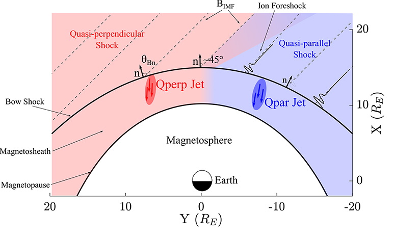
Figure 1. Sketch of the bow shock and its different configuration in the Earth's environment. An Interplanetary Magnetic Field (IMF) with an angle, approximately 45° with the normal at the nose of the bow shock is assumed. As a result, a quasi-perpendicular (θ_Bn > 45) shock takes place on the left part of the image and a quasi-parallel (θ_Bn < 45) on the right. The instabilities caused by the reflected ions in the Qpar case create the so called ion foreshock which changes drastically the properties between the Qpar shock and the Qperp one.

For the generation of Figure 1, the bow shock and magnetopause model by Chao et al. (2002) are used. The parameters used are B_z = −0.22 (nT), P_dyn = 2.15 (nPa), ${{M}}_{ms}=6.09$ and β = 2.20. These values correspond to the average conditions of the solar wind for the periods that a Qpar or a Qperp jet was found.

Classifying jets into different categories is vital to investigate the possibility of different generation mechanisms. As discussed above, there is no consensus regarding the generation of jets. By classifying jets to different bow shock configurations one can investigate both the jet properties and the associated solar wind to determine if any of the suggested mechanism apply to these subset of jets or even indicate new class-specific generation mechanisms.

1.2. Neural Networks

Neural Networks (NN) are widely used machine learning (ML) tools that are often employed to perform classification and regression tasks. Neural Networks were first introduced in 1943 (McCulloch and Pitts, 1943) and have been used for such tasks since at least 1958 (Rosenblatt, 1958). The basic principle behind NNs is that when provided with enough data, they are capable of adjusting their internal parameters in an optimal way to perform a specific task related to the data given. By iteratively parameterizing, and thus training, a neural network with error minimization techniques, it has been shown that when presented with unknown data the network is capable of accurately performing its trained task (Bishop, 1995). Lately, multi-layered (deep) neural networks have been used in various applications due to their ability to accurately model complex, and potentially unknown, relationships (Goodfellow et al., 2016; Samarasinghe, 2016).

In the last years, machine learning techniques, including neural networks, have been employed in heliospheric physics and space weather (Camporeale et al., 2018a,b). Their spectrum of application is quite broad, tackling many problems that traditional statistics or physics-based modeling techniques struggle with. Many applications of neural networks focus on predictive tasks such as the forecasting of solar flares (Florios et al., 2018; Jonas et al., 2018), Coronal Mass Ejections (CMEs) (Bobra and Ilonidis, 2016), CME arrival time (Liu et al., 2018), and geomagnetic indices (Boberg et al., 2000; Wintoft et al., 2017; Chandorkar and Camporeale, 2018). Other applications focus on space environment characterization (Shin et al., 2016; Aminalragia-Giamini et al., 2018), wave recognition (Balasis et al., 2019), and the classification of the solar wind (Camporeale et al., 2017).

In this work, we apply neural networks for a supervised learning classification task. In particular, to classify magnetosheath jets using solar wind measurements and compare the results with physics-based models. The main goal of this study is to classify jets between those originating from quasi-parallel shock transitions and those originating from quasi-perpendicular ones. By doing so, we determine whether machine learning techniques can outperform physics-based models in this task and investigate the potential connection between solar wind conditions and each jet class. Finally, as detailed below, we use parts of a pre-classified dataset of jets (Raptis et al., 2019) which we evaluate by investigating the agreement of each method with the initial classification.

2. Data

2.1. OMNIweb—Solar Wind (Upstream) Data

For the upstream conditions, which correspond to the input of the neural network, data from the OMNI database are used, available at https://omniweb.gsfc.nasa.gov/form/omni_min_def.html. The OMNI data mainly originate from the ACE spacecraft that resides in the Sun-Earth L1 point (Stone et al., 1998) and are automatically time-shifted to the Earth's bow shock nose. The time-shifted data have an 1-min resolution and take into account the bow shock location and shape (King and Papitashvili, 2005). The solar wind measurements are associated with every jet as later described, resulting in a dataset of equal length to the number of jets. This dataset is then used as input to the neural networks, consisting of the 12 physical quantities shown in Table 1.

TABLE 1

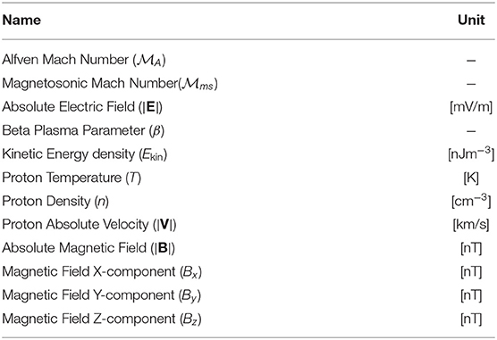
Table 1. Solar wind quantities used as input to the neural network.

2.2. MMS—Magnetosheath (Downstream) Data and Jet Database

In this work, we use a list of jets initially presented in Raptis et al. (2019). The dataset is created using in-situ measurements from the Magnetospheric Multiscale (MMS) mission during 11/2015–03/2019. For the downstream conditions and for the initial creation of the jet dataset various plasma moment and magnetic field parameters are used. The magnetic field data are taken from the fluxgate magnetometer (FGM) (Russell et al., 2016) and ion data are taken from the fast plasma investigation (FPI) (Pollock et al., 2016). Finally, the position of MMS during each jet is registered in GSE coordinates, using as unit the Earth radius (R_E = 6, 371km). This dataset provides a list of well-characterized and pre-classified jets. These are used for the training and the evaluation of the NN system, where the class of the jets serves as the desired classification output.

All the jets are required to satisfy a criterion of minimum dynamic pressure compared to the background magnetosheath plasma:

$\begin{array}{ll}{P}_{\text{dyn}}=m_p{n}_i{V}_i^2\ge {\langle P_{MSH}\rangle }_{20\text{ min}}& (1)\end{array}$

where the angular brackets indicate an average using a 20 min time moving window. m_p is the proton mass, n_i the ion number density, and V_i the ion velocity.

After each jet has been registered to the database, a classification algorithm is applied to determine its class. The main feature of the initial classification is that it uses in-situ MMS measurements to determine whether the jet originated from a quasi-parallel or a quasi-perpendicular bow shock configuration. This methodology was preferred over using solar wind data to calculate θ_Bn for several reasons. Firstly, to avoid the errors that are generated in time-lagging procedures such as the one taking place in OMNIweb database (Mailyan et al., 2008; Case and Wild, 2012). Furthermore, due to the 1-min resolution of the database, short time scale variations of the IMF are consequently undetectable. Finally, the jets are detected in the whole magnetosheath region. As a result, a time-shift on the associated solar wind values is required for every jet in order to take into account the time it took for every jet to travel inside the magnetosheath. This procedure itself is difficult to be accurately implemented and it would further increase the uncertainty of the method.

The initial dataset, therefore, relies on properties found in the magnetosheath plasma regions. In particular, the algorithm uses thresholds on ion temperature anisotropy that is found to be lower in Qpar plasma than in Qperp (Anderson et al., 1994; Fuselier et al., 1994). It also takes advantage of the fact that the magnetic field's standard deviation is observed to be higher in the Qpar plasma than in the Qperp (Formisano and Hedgecock, 1973; Luhmann et al., 1986). Finally, the main difference between the Qpar and Qperp plasma regions is the high energy ion population in the ion foreshock which only exists in the Qpar bow shock (Gosling et al., 1978; Fuselier, 2013). As a result, in-situ measurements of temperature anisotropy, magnetic field standard deviation, and high energy ion flux were used. A summary of the basic characteristics of each class is shown in Table 2. From these classes, the only ones used in this work are the Qpar (N = 860) and Qperp (N = 211) jets.

TABLE 2

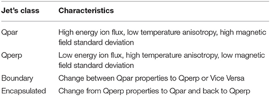
Table 2. Main properties of the classes of magnetosheath jets.

In Figure 2, an example of MMS measurements for a quasi-parallel and a quasi-perpendicular jet is shown.

FIGURE 2

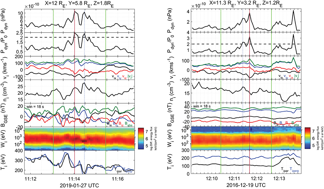
Figure 2. Left: An example of a quasi-parallel (Qpar) magnetosheath jet. Right: An example of a quasi-perpendicular (Qperp) jet. From top to bottom, ion dynamic pressure, ratio of the ion dynamic pressure to the background level, ion velocity, ion number density, magnetic field components, ion energy spectrogram and parallel and perpendicular components of ion temperature. The red vertical line shows the peak of dynamic pressure for each jet, blue vertical lines indicate the start and end point of the jet. Finally, the green lines indicate a period of time before and after the jet equal to 1 min, respectively. The velocity and magnetic field components along with the position of the spacecraft are given in GSE coordinates.

3. Methodology

3.1. Input Determination

For both the physics-based modeling and the neural networks, it is necessary to provide an input that corresponds to the same time intervals in order to have a consistent comparison. The choice of the input is nontrivial, since, as discussed in the previous section, the availability of measurements and their association to jets contains multiple errors and uncertainties. Several possible inputs were examined, by either taking average or maximum values of the conditions found within a 5, 10, or 15 min period of the jet. It was found that taking average solar wind conditions starting from 5 min before the jet up to the jet observation time provided the highest agreement to the initial classification in all presented methods. As a result, the solar wind measurements (X_u) used for each jet are defined as:

$\begin{array}{ll}{X}_u=\frac{1}{6}{\displaystyle \sum _{i=0}^5}(X_{t_{\text{jet}}-i\Delta t})& (2)\end{array}$

where, t_jet is the time the jet was observed by MMS, Δt is equal to 60 s and subscript u refers to X being an upstream quantity.

It should be noted that while the input described in Equation (2) provided the highest agreement with the initial database, it still has its limitations. Specifically, this input choice means that jets found very far away from the bow shock nose or with extremely high or low velocities will potentially not be characterized correctly.

3.2. Evaluating Jet Class With Physics-Based Modeling

In order to provide a baseline to compare the results from the neural networks, we use three different physics-based models to estimate the θ_Bn angle and distinguish between Qpar and Qperp magnetosheath jets.

3.2.1. Cone Angle Approximation

A simple approach to estimate θ_Bn is through the cone angle:

$\begin{array}{ll}{\theta }_{\text{cone}}=\text{arccos}\left(\frac{|{\text{B}}_{u,x}|}{|{\text{B}}_u|}\right)& (3)\end{array}$

where, B_u,x is the x component of the upstream magnetic field and B_u is the IMF vector. θ_cone is identical to θ_Bn at the subsolar point of the bow shock.

By calculating the cone angle, we classify the available jets. For θ_cone < 45 a jet is classified as Qpar while for θ_cone > 45 it is classified as Qperp. This method should in principle work for the majority of the jets that are found close to the subsolar point. However, the number of the jets that are in very close proximity to the subsolar point (|Y, Z_GSE| < 2R_E) is quite small (Qpar: 151/ Qperp: 108). As a result, we expect this method to perform poorly for jets found close to the flanks of the magnetosheath.

3.2.2. Coplanarity Method

Another set of methods used is the so called coplanarity methods. There is a variety of methods based on the coplanarity theorem (e.g., Paschmann and Daly, 1998). In our case, the simplest version of magnetic field coplanarity method provides the highest agreement with the initial dataset and is the one shown in this work.

Starting from Rankine–Hugoniot relations we can derive the normal vector of the bow shock as:

$\begin{array}{ll}\widehat{\text{n}}=\pm \frac{({\text{B}}_d\times {\text{B}}_u)\times \Delta \text{B}}{|({\text{B}}_d\times {\text{B}}_u)\times \Delta \text{B}|}& (4)\end{array}$

In our case, the upstream (IMF) magnetic field was taken as the average value from 5 min before the observation of the jet to the time the jet was observed (Equation 2). On the other hand, the downstream (magnetosheath) magnetic field was taken as the average value of ±2.5 min before and after the jet measurement by MMS.

This approximation should in principle be less accurate for jets found very far away from the bow shock since the jump conditions refer to points close to the shock. Furthermore, jets found at the flanks are also prone to errors since the upstream solar wind measurements are time-lagged to the bow shock nose and therefore characterize the subsolar region.

3.2.3. Bow Shock Modeling

Another method to calculate θ_Bn requires a model of the bow shock and an approximation of the origin of each jet.

Assuming that the jet does not get significantly accelerated or decelerated during its lifetime in the magnetosheath, one can use the maximum velocity vector (V) to propagate the jet backwards in time and find its point of origin at the bow shock. For the modeling of the bow shock, the model described by Chao et al. (2002) was used. It should be noted that this procedure is prone to several errors. To begin with, the position of the modeled bow shock may have a significant error compared to the real position (Merka et al., 2003; Turc et al., 2013). Furthermore, the assumption that the velocity is constant may introduce more errors. To derive a realistic bow shock model, we use the average associated solar wind conditions starting from 10 min before the jet up to 5 min after its observation by MMS. After we approximated a point of origin for each jet, the angle between the normal vector of that point and the IMF was calculated.

3.3. Evaluating Jet Class With Neural Networks

For the input of the neural networks, several inputs associated to each jet were tested. For every jet 12 solar wind measurements were used (Table 1) and were associated to it (Equation 2). From the initial number of jets (860 Qpar/211 Qperp) we exclude jets that contain corrupted data in any of the input that was used in the neural network (Table 1). As a result, the final dataset consists of 759 Qpar jets and 196 Qperp jets.

The neural network architecture, algorithm, and back-end training procedure were implemented in Python by using TensorFlow library version 2.0.0 (Abadi et al., 2015). One of the main problems of the neural network application is the treatment of the class imbalance. We are dealing with a problem where the majority class (Qpar jets) is roughly ~80% of the whole dataset. Class imbalance is a non-trivial problem to optimize in machine learning and there is no ideal solution for it (Goodfellow et al., 2016; Brownlee, 2020). In order to tackle this problem we utilized the imbalanced-learning library (Lema^ıtre et al., 2017), and used under-sampling and up-sampling techniques. In particular, we used ClusterCentroid under-sampling and SMOTE up-sampling methods on the majority of the trials (Chawla et al., 2002). It should be noted, that both under-sampling and up-sampling techniques did not increase the average accuracy of the neural network significantly. Another direct way to tackle the class imbalance problem in the training procedure is to implement a weight factor in the update of the weights and biases to compensate for the differences in the classes found in the training samples. As a result, a weighted factor was used for updating the parameters of the network when the minority class (quasi-perpendicular jets) is introduced to the network.

For the optimizer of the gradient descent algorithm, we used the Adam optimizer as implemented in the Keras library (Chollet, 2015) with a smaller learning rate of α = 0.0001 while the rest of the parameters were left at their default status. Since the neural network is tackling a binary classification problem, the error function used for the back-propagation is the binary cross-entropy loss function. In all trials and in the final architecture we also used the batch normalization technique (Ioffe and Szegedy, 2015) and parametric rectified linear units (PReLu) (He et al., 2015) in the hidden layers of the network. The final architecture of the network is shown in Figure 3 and described in Table 3.

FIGURE 3

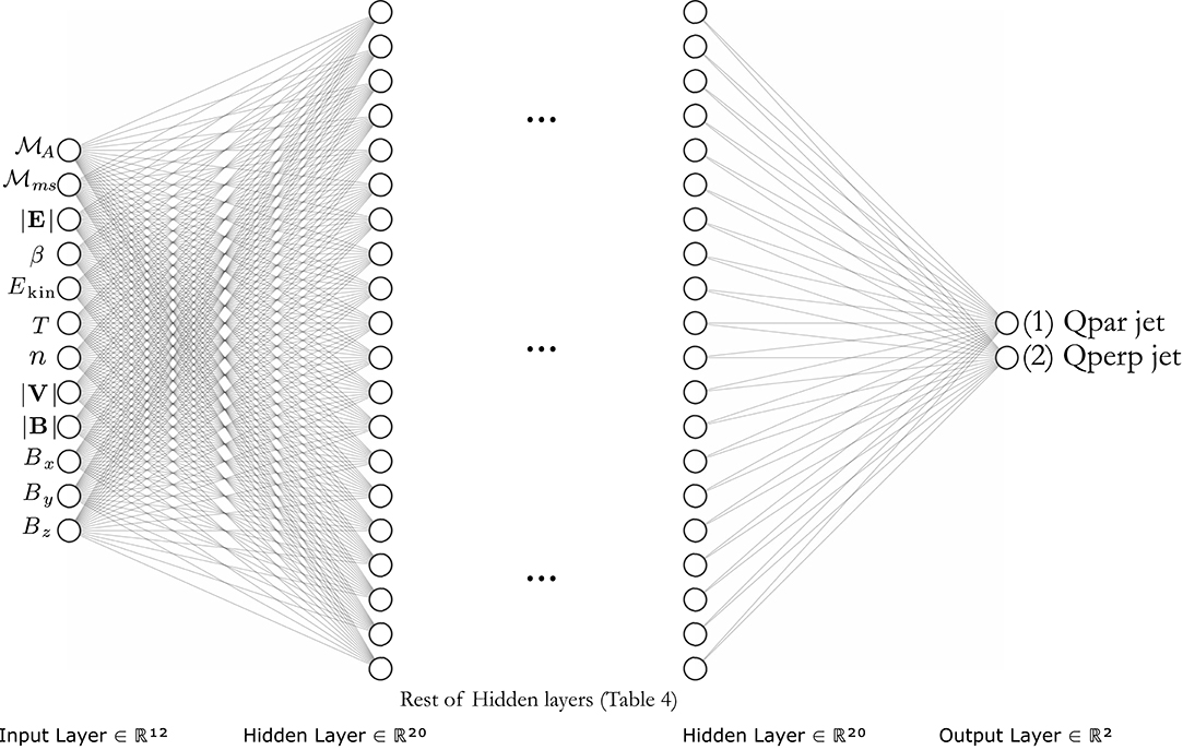
Figure 3. Basic architecture of the neural network used for the classification of the jets. The input layer shows all the quantities that were used in the neural network method. To avoid having too many nodes and neurons shown, the rest of the hidden layers are given in Table 3. The visualization was done by using a publicly available tool (LeNail, 2019) and editing its output.

TABLE 3

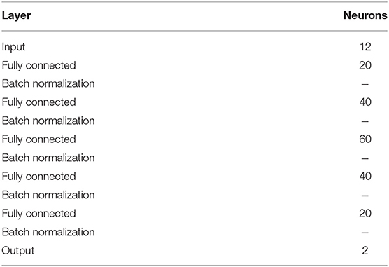
Table 3. Basic architecture of the neural network used for the classification task.

3.4. Validation Method

For the training of a neural network we have chosen to use 80% of the jets, leaving 20% available to test the accuracy of the network.

To ensure that the results are not biased from a specific division of the data into training and test sets, the process is repeated multiple times. At each iteration, the training/testing division is made randomly resulting in different subsets. Using this method, the architecture remains the same, while allowing a reasonable sampling of the, otherwise immense, space of divisions of the data into training and testing. This method is then used to evaluate the stability of the NN classifier. From each iteration, the classifying score can be calculated and the overall mean accuracy, as well as the standard deviation of the results, are direct evidence of the system's performance. In the following section results from this iterative process are shown where 100 iterations have been used.

An additional method used for the validation of the classification results is the “leave-one-out” method which produces independent classification results for each and every sample. This method is very useful when dealing with datasets of small size as it can give a good measure of the system's performance in terms of correctly classified and miss-classified cases (e.g., Aminalragia-Giamini et al., 2020). With this procedure, a neural network is trained with all the available data apart from one sample which is “left out.” After training, this one sample is input as a test set of size 1 and its class is evaluated by the network. This process iteratively evaluates all samples, setting a different one apart each time, and thus requires the training of a neural network as many times as the total number of jets, here N = 955. After its completion, this process produces 955 classification results where in each case only the sample tested did not participate in the training and every other available sample was used to produce the results. Finally, a single accuracy score can be calculated for each class which is indicative of the overall performance. The presented results of the “leave-1-out” method are the average results of three independent runs using this validation technique.

4. Results

4.1. Neural Network

An example plot of the neural network training is shown in Figure 4. The test accuracy (left) increases until ~200 epoches and as expected the test loss (right) decreases in a respective trend. Beyond the ~200 epoch point, no significant changes were observed. After using a validation set to determine the best number of epoches and batch size, we decided to use 250 epoches with a batch size equal to 100 training samples per iteration. Finally, the 80/20 training/testing division of the data results in absolute numbers in 607 Qpar jets and 157 Qperp jets for training and 152 Qpar jets and 39 Qperp jets for testing.

FIGURE 4

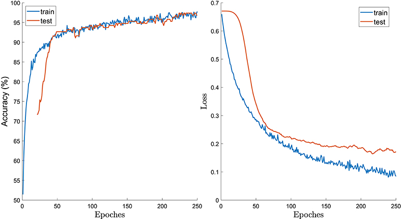
Figure 4. Example of the training procedure for a neural network run. Left: Accuracy vs. number of epoches. Right: cross-entropy loss vs. number of epoches. The results were stabilized for an epoch number of ~250. Blue lines show the behavior of the training subset while orange lines show that of the testing subset.

The classification results from 100 iterations with the random training/testing division for neural networks are shown in Figures 5, 6. Figure 5 shows the individual classification scores for Qpar and Qperp jets where it is seen that in both cases high scores with a mean accuracy of ~98.2 and ~88.9% are achieved, respectively. Specifically for the Qpar jets, the scores are tightly clustered in the ~95−100% range showing minimal standard deviation between iterations. On the other hand, the results of Qperp jets have a higher standard deviation, with accuracy scores ranging from ~75−100%. This could be due to the number of jets per class not being balanced, which provides more available information for the neural network regarding the majority class (Qpar). As a result, the testing set used for each iteration contains fewer samples which makes it possible to get worse training and test splits on each iteration. Another possible explanation is that on top of the class imbalance, due to the way Qpar and Qperp shocks form, most of Qperp jets occur much closer to the subsolar region compared to Qpar jets. As discussed previously, ~50% of Qperp jets are close to the subsolar region and the other half are further away toward the flanks. As a result, a split of data can make the result vary heavily if the training and test sample are not equally distributed.

FIGURE 5

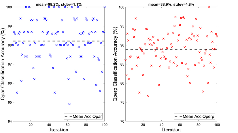
Figure 5. Accuracy of the neural network for 100 different iterations. Left: Results of the quasi-parallel class. Right: Results of the quasi-perpendicular class. The training of the shown neural networks includes the IMF vector.

FIGURE 6

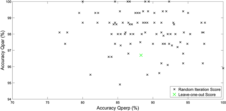
Figure 6. Accuracy of the neural network for 100 random initialization of training/test set, with every point being one iteration. The x-axis represents the accuracy in quasi-perpendicular class and ranges from 70 to 100%. On the other hand, the y-axis shows the accuracy in the quasi-parallel class and ranges from 94 to 100%. Special indication of the leave one out result is marked in green color. The training of the shown neural networks includes the IMF vector.

Figure 6 shows the resulting pairs of Qperp accuracy vs. the Qpar accuracy for each of the 100 iterations. It is seen that the distributions of the independent iterations does not exhibit any specific structure but appears random. This is important and gives confidence in the NN results since it is common in binary classification problems, such as this one, to have a competing classification problem; i.e., the higher the score for one class the lower the score for the other. This is not the case here and the differences in the respective scores appear to stem only from the random division of training/testing subsets.

Finally, in Figure 6 the classification score from the leave-one-out process can be seen with Qpar and Qperp scores equal to ~96.7 and ~88.2%, respectively. The leave-one-out process scores lie close to the mean of both the Qpar and the Qperp scores, while being slightly lower in both cases. We can speculate that the small differences may originate from the differences between the two types of validation methods. First of all, the class imbalance and the fact that resampling methods utilized in this case had to increase the dataset to a larger number of samples, could enhance the effect of class imbalance, decreasing the accuracy of the network. Furthermore, for the leave-one-out method, a validation set of 10% was used to check at which point the epoch training should be stopped. This was necessary since optimizing the epoch number or the batch size, while training with all but one jet is time consuming and outside the scope of this work. As a result, the difficulty in optimizing the hyper-parameters of the neural network for the leave-one-out case may have had a slight impact on the overall accuracy of the method.

4.2. Comparison of Neural Networks to Physics-Based Models

We now compare the classification scores obtained from the neural networks with the respective scores from the physics-based models. As seen in Table 4, neural networks outperform the physics-based modeling methods in reproducing the classification of the jets in the dataset.

TABLE 4

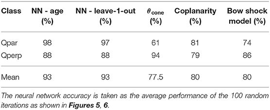
Table 4. Accuracy of each method used per class.

The simple approximation of the cone angle (Equation 3) performs very well for the Qperp class, achieving the highest score of all the methods with an accuracy of ~94% surpassing that of the neural networks. On the other hand, the cone angle method clearly underperforms in the Qpar class having the lowest score of all methods with an accuracy of only ~61%. These results show that the cone angle approximation is not well-suited for this problem. This is expected since a large portion of jets were not found in close proximity to the subsolar region.

The coplanarity method (Equation 4) performs almost equally well for the two classes with accuracy scores of ~81 and ~79% for the Qpar and Qperp classes, respectively. The accuracy scores are quite high demonstrating it is an appropriate and accurate method for this problem. However, in both classes, it is heavily outperformed by the neural networks.

Finally, using a bow shock model to calculate the θ_Bn presents an in-between case of the other two physical methods. The accuracy scores of ~74 and ~86% for the Qpar and Qperp classes, respectively, are good classification scores with a high tendency to misclassify jets as Qperp, though not as strong as in the cone-angle method. However, this method is also outperformed in both classes by the neural networks. It is interesting to note that the three physics-based methods all have mean scores, for both classes, close to ~80% implying possibly an inherent limitation due to the fact that for upstream information they only use the IMF vector. This is not true for the neural networks which can accept all the available information.

4.3. Neural Networks Without IMF (B_u) Input

After establishing the advantage of the neural network method when providing the upstream magnetic field vector (B_u), we investigate the performance of NNs even in the absence of the, in principle, vital information of the magnetic field orientation. This was done to see whether the neural network can still perform well without the IMF input that is necessary for all the other physics-based models. It should be noted, that we still used the absolute magnetic field (|B|) as input to the NN. As a result, the input in these runs consists of all the parameters shown in Table 1, except the last three which are the components of the magnetic field vector.

Similarly to the previous subsections, the results of the random train/test splits are shown in Figures 7, 8. In Figure 7, it can be seen that the average classification accuracy of both Qpar (~94.8%) and Qperp (~87.1%) class remain high even when the NN's input does not contain directional information of the IMF. Once more, the accuracy in the class of Qpar jets has a lower standard deviation than the Qperp, while in both cases the standard deviation has increased compared to the results shown in Figure 5. Again, as shown in Figure 8, there is no specific structure regarding the scores of each iteration, similarly to the previous case reported in section 4.1. The leave-one-out result is slightly lower than the average result of Qperp jets (~85.7%), while being the same as the average for the Qpar ones (~94.7%).

FIGURE 7

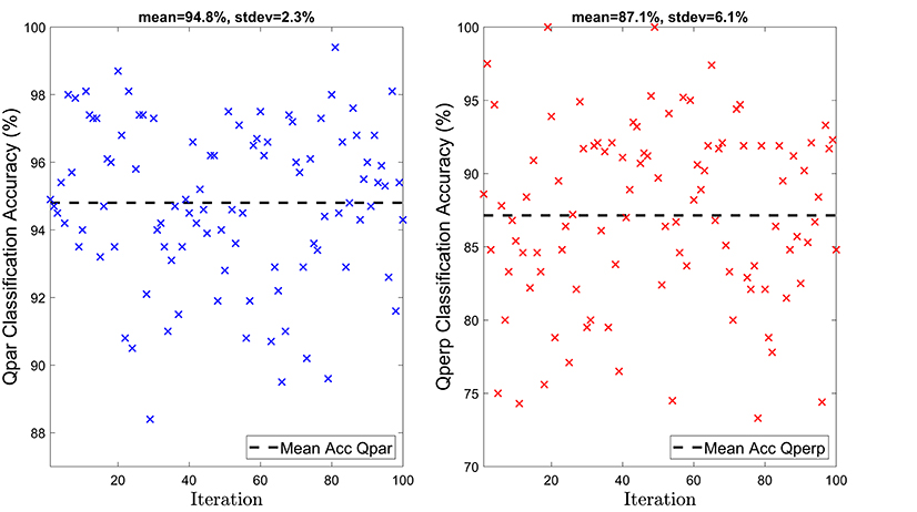
Figure 7. Accuracy of the neural network for 100 different iterations. Left: Results of the quasi-parallel class. Right: Results of the quasi-perpendicular class. The training of the shown neural networks does not includes the IMF vector.

FIGURE 8

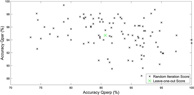
Figure 8. Accuracy of the neural network for 100 random initialization of training/test set, with every point being one iteration. The x-axis represents the accuracy in quasi-perpendicular class and ranges from 70 to 100%. On the other hand, the y-axis shows the accuracy in the quasi-parallel class and ranges from 88 to 100%. Special indication of the leave one out result is marked in green color. The training of the shown neural networks does not include the IMF vector.

4.4. Dependence of Solar Zenith Angle

After deriving a classification using all the presented methods, a possible link between the misclassified jets and their position in the magnetosheath is investigated. As discussed previously, the solar wind measurements provided as input for all methods, characterize the subsolar region and are not ideal for the characterization of the flanks. As a result, we investigate if this effect is shown in the classification results of each method.

In Figure 9, we present the probability of jets appearing for difference solar zenith angles. There are 4 histograms per jet class that correspond to the 4 presented methods of classifications. On each histogram, there are 3 plots representing the total number of jets (blue), the misclassified jets (red) and the normalized misclassified cases (black). Figure 9A shows the results of the Qpar jets while Figure 9B shows the Qperp jets. It can be seen that most cases of misclassification occur for angles close to the subsolar region (≤ 30°). However, when looking at the normalized misclassified rates (black line), it appears that when taking into account the overall number of jets, the relative misclassification rate is much higher close to the flanks (≥ 30°).

FIGURE 9

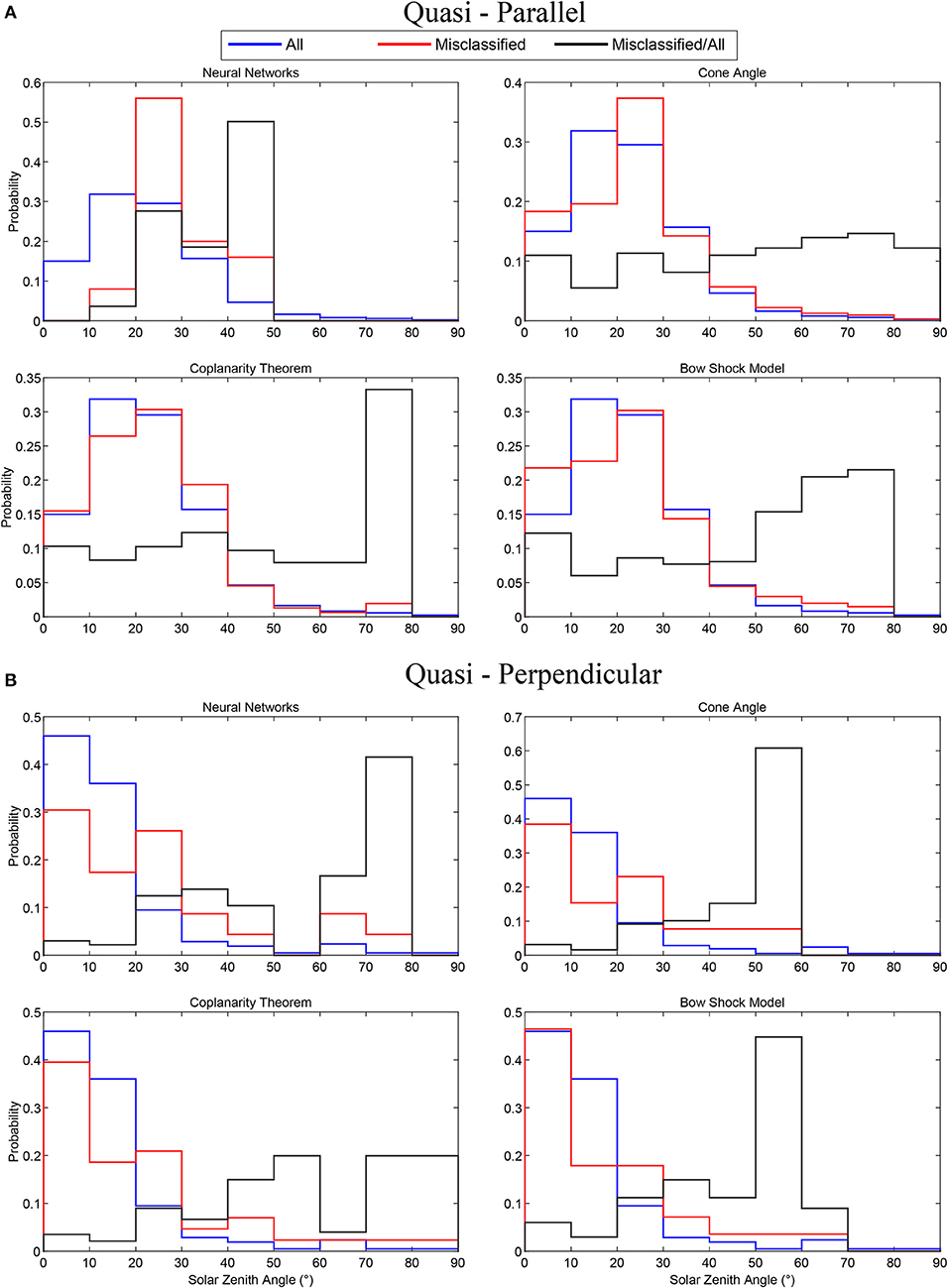
Figure 9. Histograms showing the relative position of jets in the magnetosheath (solar zenith angle). Blue lines represent the whole number of jets, Red show the misclassified jets and black show the misclassified cases normalized over the whole number of jets. (A): Quasi-parallel jets (n = 860). (B): Quasi-perpendicular jets (n = 211).

5. Discussion and Conclusions

From the results of the neural network application (Figures 5, 6, and Table 4), it is clearly shown that neural networks are capable of reproducing the results of the initial database with greater accuracy than the alternative physics-based models.

The different results for each method likely originates from the different properties the associated solar wind values between the Qpar and Qperp jets (Raptis et al., 2019). As shown in Figure 4 of Raptis et al. (2019), the velocity of Qperp jets is much lower than that of the Qpar jets, with the first having an average absolute ion velocity of ~100 km/s, while Qpar have ~230 km/s. Furthermore, it was shown that the average solar wind velocity under which Qpar jets were found was 〈V_{SW, ||Jets}〉 ≈ 495 km/s with a standard deviation of σ_{||, Jets} = 96 km/s. On the other hand for the Qperp jet, 〈V_{SW, ⊥Jets}〉 ≈ 400 km/s with σ_{⊥, Jets} = 46 km/s. These differences in the velocity of the jets can have a large effect on the final results since they not only affect the input parameter space (solar wind velocity) but also the association timing (5-min average) differently for every class.

To begin with, the cone angle approximation is working effectively only for the Quasi-perpendicular jets. This is most likely because the majority of them were found close to the subsolar region. Another reason could be that most Qperp jets have a lower average velocity (Raptis et al., 2019), that along with the proximity to the subsolar region may make the 5-min average values used for the modeling more accurate. The better overall results of the bow shock modeling method originate from the estimation of the bow shock normal vector $\widehat{\mathbf{\text{n}}}$. By finding a point of origin for each jet, many cases that were found closer to the flanks of the magnetosheath region were correctly classified. Finally, the coplanarity method, while still producing overall worse results than the neural network, showed that a significant part of the jets can be classified using this approach. As shown in Figure 9, the majority of the jets, and especially Qperp jets occur close to the subsolar region (≤ 30°). However, in all the presented methods the misclassified cases occur mainly close to the flanks. This could originate from the poor characterization of OMNIweb data regarding phenomena that occur close to the flanks. In particular, OMNIweb has a poor capability of catching intervals of quasi-radial IMF (Bier et al., 2014; Suvorova and Dmitriev, 2016). Under quasi-radial IMF there is a quasi-perpendicular shock forming close to the flanks. As a result, Qperp jets found close to the flanks are probably not characterized well enough by the available solar wind measurements that were given as input to all the methods.

The superiority of the neural network provides indirect support to the initial dataset. This is achieved because the input of the neural network was independent of the one used in the initial classification. In particular, the initial database was classified using only magnetosheath (downstream) data, while the neural network input contained only solar wind (upstream) information. According to Figure 9, the highest evaluation accuracy was obtained for jets found in close vicinity of the subsolar region. As already stated previously, the OMNIweb database provides measurements that correspond to the subsolar region and therefore are not ideal to characterize the flank regions. Furthermore, the jets found very far from the bow shock could have taken a longer time to propagate in the magnetosheath region, making the choice of 5-min averaging dubious. A better estimation of the jet travel time from the bow shock to its observation point could possibly increase the accuracy of all the presented methods. These results show that the choice of using in-situ measurements for the determination of jets' class may indeed provide more accurate results while not limiting the classification procedure to periods of times that upstream data are available (Raptis et al., 2019). There are many jets that were found far away from the subsolar region (Y_GSE > 5R_E) that were systematically misclassified by the physics-based methods. However, a good portion of them was correctly classified by the neural network approach. As previously discussed, the main problem with jets that are found at the flanks of the magnetosheath is that the measurements taken from the solar wind do not accurately characterize this region. Furthermore, the time propagation error along with the error of the origin position is greatly enhanced the further away a jet is found from the bow shock. Nevertheless, due to the availability of such cases, the neural network was able to recognize peculiar cases, “train” for them, and correctly identify a significant portion of them. Table 6, shows the number of misclassifications done per method grouped in three ranges, these close to the subsolar region ([0−30]°) these further away from the subsolar ([30−50]°) and the ones far toward the flanks of the magnetosheath ([50−90]°). It is clear, that neural networks not only outperform the rest of the methods in the regions where jets are found more frequently but also in the not so common cases of flank jets.

To increase the accuracy of the neural network, one could in principle train two different NNs to tackle the different characterization of subsolar jets and flank jets. Then by utilizing ensemble learning methods, each network could work on its appropriate dataset possibly providing superior combined results. This task is not trivial since the boundary of where a subsolar region starts and ends is not sharp. Furthermore, depending on the properties of the jet, the association of solar wind measurements is an extremely complicated task. In this work, we used 5-min average values that while characterizing the majority of the events, they may fail to do so if a jet has very high velocities or if a significant part of its velocity lies in the yz plane, which could mean that it traveled in the magnetosheath for a longer period of time. All the above, along with the determination of the rest of the classes, shown in the presented database (Table 2) are planned to be done in future studies.

From a physical point of view, the most interesting result is perhaps the fact that neural networks maintained a very high accuracy even in the absence of the directional information of the IMF (Figures 7, 8 and Table 5). This could be interpreted in several different ways. The most direct one is that the neural networks take advantage of the fact that in the initial database, the jets found in quasi-perpendicular plasma have on average a lower velocity and density than the jets found in the quasi-parallel magnetosheath. It is, however, not yet fully understood if this is the result of an observational bias or of a real physical mechanism (Raptis et al., 2019). The observational bias here would be that for conditions of low velocity and density, the threshold of finding a jet is easier to be satisfied (Equation 1). This would in principle allow jets that are found in the quasi-perpendicular plasma to occur primarily under low velocity and density solar wind. On the other hand, such a bias is not likely to fully explain the shown results. The conditions under which Qperp jets are found could originate from a physical process that makes Qperp jets more likely to occur under specific solar wind conditions, regardless of the IMF direction. If the latter is true, it means that an investigation of solar wind classes (e.g., Habbal et al., 1997; Camporeale et al., 2017) could give insight as to whether each jet class (Table 2) occurs under different conditions or if specific conditions simply favor the formation of one class over the other. A final possible explanation is that directional information of the IMF is “hidden” in various quantities that were used for the training of the neural network. This, in turn, would allow the non-linear relationship generated by the network to accurately find the correct class of the jets by utilizing such previously undetectable information.

TABLE 5

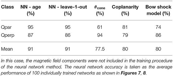
Table 5. Accuracy of each method used per class.

TABLE 6

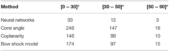
Table 6. Number of misclassifications grouped in different solar zenith angles for every classification method.

Neural Networks were shown to be a powerful method for the classification of magnetosheath jets. They outperformed the physics-based methods used in distinguishing between quasi-parallel and quasi-perpendicular jets. The results here, also indicate that upstream solar wind properties are sufficient to predict the class of the jets even without including the magnetic field vector. Last but not least, machine learning approaches, such as this one, can be generalized and applied to several satellite missions and space environments.

Data Availability Statement

MMS data are available at the MMS Science Data Center (https://lasp.colorado.edu/mms/sdc). OMNIweb Data are available at https://omniweb.gsfc.nasa.gov/form/omni_min.html. Finally, the time of observation, the initial classification and the classification done by the neural networks and the three physical methods can be found in the Supplementary Material or in the associated data repository (Raptis et al., 2020).

Author Contributions

SR and SA-G performed the data analysis. SR wrote the paper with contributions from SA-G, TK, and ML. All the authors contributed to drafting and revising the paper. All the authors contributed to the interpretation of the data.

Funding

SR and TK acknowledge support from the Swedish National Space Board (SNSA grant 90/17).

Conflict of Interest

The authors declare that the research was conducted in the absence of any commercial or financial relationships that could be construed as a potential conflict of interest.

Acknowledgments

We thank the MMS team for providing data and support https://lasp.colorado.edu/mms/sdc/public/. Furthermore, we acknowledge use of NASA/GSFC's Space Physics Data Facility's OMNIWeb service, and OMNI data. OMNI High-resolution data are available through https://omniweb.gsfc.nasa.gov/form/omni_min.html.

Supplementary Material

The Supplementary Material for this article can be found online at: https://www.frontiersin.org/articles/10.3389/fspas.2020.00024/full#supplementary-material

References

Abadi, M., Agarwal, A., Barham, P., Brevdo, E., Chen, Z., Citro, C., et al. (2015). TensorFlow: Large-Scale Machine Learning on Heterogeneous Systems. Software available online at: tensorflow.org

Google Scholar

Amata, E., Savin, S., Ambrosino, D., Bogdanova, Y., Marcucci, M., Romanov, S., et al. (2011). High kinetic energy density jets in the Earth's magnetosheath: a case study. Planet. Space Sci. 59, 482–494. doi: 10.1016/j.pss.2010.07.021

CrossRef Full Text | Google Scholar

Aminalragia-Giamini, S., Jiggens, P., Anastasiadis, A., Sandberg, I., Aran, A., Vainio, R., et al. (2020). Prediction of solar proton event fluence spectra from their peak flux spectra. J. Space Weather Space Clim. 10:1. doi: 10.1051/swsc/2019043

CrossRef Full Text | Google Scholar

Aminalragia-Giamini, S., Papadimitriou, C., Sandberg, I., Tsigkanos, A., Jiggens, P., Evans, H., et al. (2018). Artificial intelligence unfolding for space radiation monitor data. J. Space Weather Space Clim. 8:A50. doi: 10.1051/swsc/2018041

CrossRef Full Text | Google Scholar

Anderson, B. J., Fuselier, S. A., Gary, S. P., and Denton, R. E. (1994). Magnetic spectral signatures in the earth's magnetosheath and plasma depletion layer. J. Geophys. Res. Space Phys. 99, 5877–5891. doi: 10.1029/93JA02827

CrossRef Full Text | Google Scholar

Archer, M., Hietala, H., Hartinger, M., Plaschke, F., and Angelopoulos, V. (2019). Direct observations of a surface eigenmode of the dayside magnetopause. Nat. Commun. 10:615. doi: 10.1038/s41467-018-08134-5

PubMed Abstract | CrossRef Full Text | Google Scholar

Archer, M., Horbury, T., and Eastwood, J. (2012). Magnetosheath pressure pulses: Generation downstream of the bow shock from solar wind discontinuities. J. Geophys. Res. Space Phys. 117:A5. doi: 10.1029/2011JA017468

CrossRef Full Text | Google Scholar

Archer, M. O., and Horbury, T. S. (2013). Magnetosheath dynamic pressure enhancements: occurrence and typical properties. Ann. Geophys. 31, 319–331. doi: 10.5194/angeo-31-319-2013

CrossRef Full Text | Google Scholar

Balasis, G., Aminalragia-Giamini, S., Papadimitriou, C., Daglis, I. A., Anastasiadis, A., and Haagmans, R. (2019). A machine learning approach for automated ulf wave recognition. J. Space Weather Space Clim. 9:A13. doi: 10.1051/swsc/2019010

CrossRef Full Text | Google Scholar

Balogh, A., and Treumann, R. A. (2013). Physics of Collisionless Shocks: Space Plasma Shock Waves. New York, NY: Springer. doi: 10.1007/978-1-4614-6099-2

CrossRef Full Text | Google Scholar

Baumjohann, W., and Treumann, R. A. (2012). Basic Space Plasma Physics. London: World Scientific Publishing Company. doi: 10.1142/p850

CrossRef Full Text | Google Scholar

Bier, E. A., Owusu, N., Engebretson, M. J., Posch, J. L., Lessard, M. R., and Pilipenko, V. A. (2014). Investigating the IMF cone angle control of pc3-4 pulsations observed on the ground. J. Geophys. Res. Space Phys. 119, 1797–1813. doi: 10.1002/2013JA019637

CrossRef Full Text | Google Scholar

Bishop, C. M. (1995). Neural Networks for Pattern Recognition. Oxford University Press. doi: 10.1201/9781420050646.ptb6

CrossRef Full Text | Google Scholar

Boberg, F., Wintoft, P., and Lundstedt, H. (2000). Real time KP predictions from solar wind data using neural networks. Phys. Chem. Earth C Solar Terres. Planet. Sci. 25, 275–280. doi: 10.1016/S1464-1917(00)00016-7

CrossRef Full Text | Google Scholar

Bobra, M. G., and Ilonidis, S. (2016). Predicting coronal mass ejections using machine learning methods. Astrophys. J. 821:127. doi: 10.3847/0004-637X/821/2/127

CrossRef Full Text | Google Scholar

Brownlee, J. (2020). Imbalanced Classification with Python: Better Metrics, Balance Skewed Classes, Cost-Sensitive Learning. Machine Learning Mastery. Available online at: https://books.google.be/books?id=jaXJDwAAQBAJ

Google Scholar

Camporeale, E., Carè, A., and Borovsky, J. E. (2017). Classification of solar wind with machine learning. J. Geophys. Res. Space Phys. 122, 10,910–10,920. doi: 10.1002/2017JA024383

CrossRef Full Text | Google Scholar

Camporeale, E., Wing, S., and Johnson, J. (2018b). Space weather in the machine learning era. EOS 99. doi: 10.1029/2018EO101897

CrossRef Full Text | Google Scholar

Camporeale, E., Wing, S., and Johnson, J. (eds.),., (2018a). Machine Learning Techniques for Space Weather. Elsevier, p. 454. Availabe online at: https://www.elsevier.com/books/machine-learning-techniques-for-space-weather/camporeale/978-0-12-811788-0

Google Scholar

Case, N., and Wild, J. (2012). A statistical comparison of solar wind propagation delays derived from multispacecraft techniques. J. Geophys. Res. Space Phys. 117:A2. doi: 10.1029/2011JA016946

CrossRef Full Text | Google Scholar

Chandorkar, M., and Camporeale, E. (2018). “Probabilistic forecasting of geomagnetic indices using Gaussian process models.” in Machine Learning Techniques for Space Weather, eds E. Camporeale, S. Wing, and J. R. Johnson (Elsevier), 237–258. doi: 10.1016/B978-0-12-811788-0.00009-3

CrossRef Full Text | Google Scholar

Chao, J., Wu, D., Lin, C.-H., Yang, Y.-H., Wang, X., Kessel, M., et al. (2002). “Models for the size and shape of the earth's magnetopause and bow shock,” in Cospar Colloquia Series, Vol. 12, ed L.-H. Lyu (Taipei: Elsevier), 127–135. doi: 10.1016/S0964-2749(02)80212-8

CrossRef Full Text | Google Scholar

Chawla, N. V., Bowyer, K. W., Hall, L. O., and Kegelmeyer, W. P. (2002). Smote: synthetic minority over-sampling technique. J. Artif. Intell. Res. 16, 321–357. doi: 10.1613/jair.953

CrossRef Full Text | Google Scholar

Chollet, F. (2015). Keras. Available online at: https://github.com/fchollet/keras

Google Scholar

Florios, K., Kontogiannis, I., Park, S.-H., Guerra, J. A., Benvenuto, F., Bloomfield, D. S., et al. (2018). Forecasting solar flares using magnetogram-based predictors and machine learning. Solar Phys. 293:28. doi: 10.1007/s11207-018-1250-4

CrossRef Full Text | Google Scholar

Formisano, V., and Hedgecock, P. (1973). Solar wind interaction with the earth's magnetic field: 3. On the earth's bow shock structure. J. Geophys. Res. 78, 3745–3760. doi: 10.1029/JA078i019p03745

CrossRef Full Text | Google Scholar

Fuselier, S. A. (2013). Suprathermal Ions Upstream and Downstream from the Earth's Bow Shock. Washington, DC: American Geophysical Union (AGU). doi: 10.1029/GM081p0107

PubMed Abstract | CrossRef Full Text | Google Scholar

Fuselier, S. A., Anderson, B. J., Gary, S. P., and Denton, R. E. (1994). Inverse correlations between the ion temperature anisotropy and plasma beta in the earth's quasi-parallel magnetosheath. J. Geophys. Res. Space Phys. 99, 14931–14936. doi: 10.1029/94JA00865

CrossRef Full Text | Google Scholar

Giacalone, J., and Jokipii, J. R. (2007). Magnetic field amplification by shocks in turbulent fluids. Astrophys. J. Lett. 663:L41. doi: 10.1086/519994

CrossRef Full Text | Google Scholar

Goodfellow, I., Bengio, Y., and Courville, A. (2016). Deep Learning. Cambridge, MA: MIT press.

PubMed Abstract | Google Scholar

Gosling, J., Asbridge, J., Bame, S., Paschmann, G., and Sckopke, N. (1978). Observations of two distinct populations of bow shock ions in the upstream solar wind. Geophys. Res. Lett. 5, 957–960. doi: 10.1029/GL005i011p00957

CrossRef Full Text | Google Scholar

Gunell, H., Wieser, G. S., Mella, M., Maggiolo, R., Nilsson, H., Darrouzet, F., et al. (2014). Waves in high-speed plasmoids in the magnetosheath and at the magnetopause. Ann. Geophys. 32, 991–1009. doi: 10.5194/angeo-32-991-2014

CrossRef Full Text | Google Scholar

Gutynska, O., Sibeck, D., and Omidi, N. (2015). Magnetosheath plasma structures and their relation to foreshock processes. J. Geophys. Res. Space Phys. 120, 7687–7697. doi: 10.1002/2014JA020880

CrossRef Full Text | Google Scholar

Habbal, S., Woo, R., Fineschi, S., O'Neal, R., Kohl, J., Noci, G., et al. (1997). Origins of the slow and the ubiquitous fast solar wind. Astrophys. J. Lett. 489:L103. doi: 10.1086/310970

CrossRef Full Text | Google Scholar

Han, D.-S., Hietala, H., Chen, X.-C., Nishimura, Y., Lyons, L. R., Liu, J.-J., et al. (2017). Observational properties of dayside throat aurora and implications on the possible generation mechanisms. J. Geophys. Res. Space Phys. 122, 1853–1870. doi: 10.1002/2016JA023394

CrossRef Full Text | Google Scholar

He, K., Zhang, X., Ren, S., and Sun, J. (2015). “Delving deep into rectifiers: surpassing human-level performance on imagenet classification,” in Proceedings of the IEEE International Conference on Computer Vision, 1026–1034. doi: 10.1109/ICCV.2015.123

CrossRef Full Text | Google Scholar

Hietala, H., Laitinen, T. V., Andréeová, K., Vainio, R., Vaivads, A., Palmroth, M., et al. (2009). Supermagnetosonic jets behind a collisionless quasiparallel shock. Phys. Rev. Lett. 103:245001. doi: 10.1103/PhysRevLett.103.245001

PubMed Abstract | CrossRef Full Text | Google Scholar

Hietala, H., Phan, T., Angelopoulos, V., Oieroset, M., Archer, M., Karlsson, T., et al. (2018). In situ observations of a magnetosheath high-speed jet triggering magnetopause reconnection. Geophys. Res. Lett. 45, 1732–1740. doi: 10.1002/2017GL076525

CrossRef Full Text | Google Scholar

Hietala, H., and Plaschke, F. (2013). On the generation of magnetosheath high-speed jets by bow shock ripples. J. Geophys. Res. Space Phys. 118, 7237–7245. doi: 10.1002/2013JA019172

PubMed Abstract | CrossRef Full Text | Google Scholar

Ioffe, S., and Szegedy, C. (2015). “Batch normalization: accelerating deep network training by reducing internal covariate shift,” in: Proceedings of the 32nd International Conference on International Conference on Machine Learning, Vol. 37 (Lille: JMLR.org), 448–456. doi: 10.5555/3045118.3045167

CrossRef Full Text | Google Scholar

Jonas, E., Bobra, M., Shankar, V., Hoeksema, J. T., and Recht, B. (2018). Flare prediction using photospheric and coronal image data. Solar Phys. 293:48. doi: 10.1007/s11207-018-1258-9

CrossRef Full Text | Google Scholar

Karlsson, T., Brenning, N., Nilsson, H., Trotignon, J.-G., Vallières, X., and Facsko, G. (2012). Localized density enhancements in the magnetosheath: three-dimensional morphology and possible importance for impulsive penetration. J. Geophys. Res. Space Phys. 117:A3. doi: 10.1029/2011JA017059

CrossRef Full Text | Google Scholar

Karlsson, T., Kullen, A., Liljeblad, E., Brenning, N., Nilsson, H., Gunell, H., et al. (2015). On the origin of magnetosheath plasmoids and their relation to magnetosheath jets. J. Geophys. Res. Space Phys. 120, 7390–7403. doi: 10.1002/2015JA021487

CrossRef Full Text | Google Scholar

King, J., and Papitashvili, N. (2005). Solar wind spatial scales in and comparisons of hourly wind and ace plasma and magnetic field data. J. Geophys. Res. Space Phys. 110:A2. doi: 10.1029/2004JA010649

CrossRef Full Text | Google Scholar

Lemaître, G., Nogueira, F., and Aridas, C. K. (2017). Imbalanced-learn: a python toolbox to tackle the curse of imbalanced datasets in machine learning. J. Mach. Learn. Res. 18, 559–563. Available online at: http://jmlr.csail.mit.edu/papers/v18/16-365.html

Google Scholar

LeNail, A. (2019). NN-SVG: Publication-ready neural network architecture schematics. J. Open Source Softw. 4:747. doi: 10.21105/joss.00747

CrossRef Full Text | Google Scholar

Liu, J., Ye, Y., Shen, C., Wang, Y., and Erdélyi, R. (2018). A new tool for CME arrival time prediction using machine learning algorithms: cat-puma. Astrophys. J. 855:109. doi: 10.3847/1538-4357/aaae69

CrossRef Full Text | Google Scholar

Luhmann, J., Russell, C., and Elphic, R. (1986). Spatial distributions of magnetic field fluctuations in the dayside magnetosheath. J. Geophys. Res. Space Phys. 91, 1711–1715. doi: 10.1029/JA091iA02p01711

CrossRef Full Text | Google Scholar

Mailyan, B., Munteanu, C., and Haaland, S. (2008). What is the best method to calculate the solar wind propagation delay? Ann. Geophys. 26, 2383–2394, doi: 10.5194/angeo-26-2383-2008

CrossRef Full Text | Google Scholar

McCulloch, W. S., and Pitts, W. (1943). A logical calculus of the ideas immanent in nervous activity. Bull. Math. Biophys. 5, 115–133. doi: 10.1007/BF02478259

CrossRef Full Text | Google Scholar

Merka, J., Szabo, A., Narock, T., King, J., Paularena, K., and Richardson, J. (2003). A comparison of IMP 8 observed bow shock positions with model predictions. J. Geophys. Res. Space Phys. 108:A2. doi: 10.1029/2002JA009384

CrossRef Full Text | Google Scholar

Němeček, Z., Šafránková, J., Přech, L., Sibeck, D., Kokubun, S., and Mukai, T. (1998). Transient flux enhancements in the magnetosheath. Geophys. Res. Lett. 25, 1273–1276. doi: 10.1029/98GL50873

CrossRef Full Text | Google Scholar

Paschmann, G., and Daly, P. W. (1998). Analysis Methods for Multi-spacecraft Data. Bern.

Google Scholar

Plaschke, F., Hietala, H., Archer, M., Blanco-Cano, X., Kajdič, P., Karlsson, T., et al. (2018). Jets downstream of collisionless shocks. Space Sci. Rev. 214:81. doi: 10.1007/s11214-018-0516-3

CrossRef Full Text | Google Scholar

Pollock, C., Moore, T., Jacques, A., Burch, J., Gliese, U., Saito, Y., et al. (2016). Fast plasma investigation for magnetospheric multiscale. Space Sci. Rev. 199, 331–406. doi: 10.1007/s11214-016-0245-4

CrossRef Full Text | Google Scholar

Raptis, S., Aminalragia-Giamini, S., Karlsson, T., and Lindberg, M. (2020). Magnetosheath Jets (Qpar-Qperp) Classification [Data set]. Front. Astron. Space Sci. doi: 10.5281/zenodo.3746592

CrossRef Full Text | Google Scholar

Raptis, S., Karlsson, T., Plaschke, F., Kullen, A., and Lindqvist, P.-A. (2019). Classifying magnetosheath jets using mms - statistical properties. Earth Space Sci. Open Arch. 41. doi: 10.1002/essoar.10501493.2

CrossRef Full Text | Google Scholar

Rosenblatt, F. (1958). The perceptron: a probabilistic model for information storage and organization in the brain. Psychol. Rev. 65:386. doi: 10.1037/h0042519

PubMed Abstract | CrossRef Full Text | Google Scholar

Russell, C., Anderson, B., Baumjohann, W., Bromund, K., Dearborn, D., Fischer, D., et al. (2016). The magnetospheric multiscale magnetometers. Space Sci. Rev. 199, 189–256. doi: 10.1007/s11214-014-0057-3

CrossRef Full Text | Google Scholar

Samarasinghe, S. (2016). Neural Networks for Applied Sciences and Engineering: From Fundamentals to Complex Pattern Recognition. New York, NY: Auerbach publications.

Google Scholar

Schwartz, S. J., and Burgess, D. (1991). Quasi-parallel shocks: a patchwork of three-dimensional structures. Geophys. Res. Lett. 18, 373–376. doi: 10.1029/91GL00138

CrossRef Full Text | Google Scholar

Schwartz, S. J., Burgess, D., Wilkinson, W. P., Kessel, R. L., Dunlop, M., and Lühr, H. (1992). Observations of short large-amplitude magnetic structures at a quasi-parallel shock. J. Geophys. Res. Space Phys. 97, 4209–4227. doi: 10.1029/91JA02581

CrossRef Full Text | Google Scholar

Shin, D.-K., Lee, D.-Y., Kim, K.-C., Hwang, J., and Kim, J. (2016). Artificial neural network prediction model for geosynchronous electron fluxes: dependence on satellite position and particle energy. Space Weather 14, 313–321. doi: 10.1002/2015SW001359

CrossRef Full Text | Google Scholar

Stone, C. E., Frandsen, A. M., Mewaldt, R., Christian, E., Margolies, D., Ormes, J., et al. (1998). The advanced composition explorer mission. Space Sci. Rev. 86, 1–22. doi: 10.1007/978-94-011-4762-0_1

CrossRef Full Text | Google Scholar

Suvorova, A., and Dmitriev, A. (2016). On magnetopause inflation under radial IMF. Adv. Space Res. 58, 249–256. doi: 10.1016/j.asr.2015.07.044

CrossRef Full Text | Google Scholar

Turc, L., Fontaine, D., Savoini, P., Hietala, H., and Kilpua, E. K. J. (2013). A comparison of bow shock models with cluster observations during low alfvén mach number magnetic clouds. Ann. Geophys. 31, 1011–1019. doi: 10.5194/angeo-31-1011-2013

CrossRef Full Text | Google Scholar

Turner, D. L., Shprits, Y., Hartinger, M., and Angelopoulos, V. (2012). Explaining sudden losses of outer radiation belt electrons during geomagnetic storms. Nat. Phys. 8:208. doi: 10.1038/nphys2185

CrossRef Full Text | Google Scholar

Wilson, L. III. (2016). “Low frequency waves at and upstream of collisionless shocks,” in Low-Frequency Waves in Space Plasmas eds A. Keiling, D. H. Lee, and V. Nakariakov (Hoboken, NJ: John Wiley & Sons, Inc.), 269–291. doi: 10.1002/9781119055006.ch16

CrossRef Full Text | Google Scholar

Wintoft, P., Wik, M., Matzka, J., and Shprits, Y. (2017). Forecasting KP from solar wind data: input parameter study using 3-hour averages and 3-hour range values. J. Space Weather Space Clim. 7:A29. doi: 10.1051/swsc/2017027

CrossRef Full Text | Google Scholar

Xiang, Z., Ni, B., Zhou, C., Zou, Z., Gu, X., Zhao, Z., et al. (2016). Multi-satellite simultaneous observations of magnetopause and atmospheric losses of radiation belt electrons during an intense solar wind dynamic pressure pulse. Ann. Geophys. 34, 493–509. doi: 10.5194/angeo-34-493-2016

CrossRef Full Text | Google Scholar