Less Is Better. Avoiding Redundant Measurements in Studies on Wild Birds in Accordance to the Principles of the 3Rs

Introduction

Unlike in research using laboratory and farm/domestic animals, access to animals in wildlife research is often highly unpredictable. No matter how skillful and well-informed the staff is, it takes favorable circumstances and a stroke of good luck to e.g., dart a moose or catch a migrant bird. Once the animal is finally available, the researcher is tempted to make utmost use of the occasion, and thus, measure and sample “as much as possible.” When challenged, the use of the individual animal beyond the core purpose of the study could easily be motivated with e.g., data sharing and bio-banking in an a posteriori manner. How does such opportunistic sampling behavior match the legal and moral requirements of the use of animals in research?

The Principles of the 3Rs are at the core of modern regulations of the use of animals in research and education (1–3). Originally formulated by Russell and Burch (4), the Principles of the 3Rs (“the 3Rs”) prescribe a continuous process aiming to Replace live animals with other study systems (e.g., cell cultures or computer models), to Reduce the numbers of animals used without jeopardizing the quality of the research and, finally, Refine the conditions for the individual animals truly needed for the experiment. The 3Rs apply independently from legal definitions of “animals used in experiments and teaching” and thus, the requirements for approval by an Ethical Committee on Animal Experiments (“ECAE”). In addition to positive effects on animal welfare, the implementation of the 3Rs is known to improve research quality through better planning and the development of novel methods and practices [e.g., (5)].

The 3Rs are now firmly rooted and routinely implemented in laboratory research (6, 7). Also in research based on the use of farm and domestic animals, the 3Rs are rapidly gaining momentum (8). In both fields, a predictable research environment facilitates a strict application of methods and protocols, high-quality care taking and housing, and properly organized and educated staff. The main body of the EU and Swedish national regulations for animals used in research were developed for these research environments, but they also apply to wildlife research (2, 9). In their review of the implementation of the 3Rs in wildlife research, (10) sorted out the challenges and possibilities for bringing wildlife research in par with practices in the laboratory and the farm. They concluded that raised 3R-awareness and field-adapted methods and protocols were important factors for successful implementation.

In most wildlife research, the animals are the object of study rather than a means to study other phenomena (e.g., toxicity or medical treatment). For this reason, the wildlife researcher has an inherently genuine interest in the well-being and functioning of the included individuals. How well this interest is materialized depends on the species-specific veterinary knowledge and skills of the research team, as well as the organization and the toolbox of the operation. In ornithology, unpaid volunteers and amateur researchers do most of the fieldwork (11–13), and their competence in the field of animal welfare, the 3Rs and research planning is often insufficient.

The numbers of wild birds subjected to scientific experimentation are unknown. For e.g., Sweden, which has a special definition of animals used in scientific experimentation (14), the official statistics for animals used in research (15) do not separate numbers for different research environments. Together with colleagues, I have estimated the number of wild birds used in research in Sweden to be c. 10,000 annually. To this number, c. 300,000 birds subject to “normal” ringing should be added (16). Bird ringing does not require ECAE approval in Sweden and most other countries.

Bird ringing not only involves catching and putting a metal ring around the leg of a bird, but also collecting data on weight, wing length, molt patterns, fat scores, etc. These all add to the overall time the bird is held captive and the level of human-induced stress the individual bird is exposed to. Handling times and levels of invasiveness are assumed to be valid proxies for negative impacts on welfare and fitness [e.g., (17–19)]. Consequently, a reduction of handling time and/or avoidance of particularly invasive treatments would improve the well-being of the wild birds used in research. From a 3R point of view, the fringe benefit of each additional measurement or treatment must be shown to out-weigh the negative effects.

Large avian herbivores (e.g., swans, geese, and cranes) wintering in the agricultural landscapes of temperate Eurasia and North America have increased dramatically in numbers over the last decades (20, 21). The Bean Goose Anser fabalis is one of the few exceptions to this general trend, with a stable population at best (21, 22). The Bean Goose has a complex and long-debated population structure (23–28) and several subspecies and sub-populations are in marked decline (29, 30). Throughout its range, the Bean Goose is subject to both regulated and illegal hunting and, when in conflict with agricultural interests, protective shooting, and scaring (14, 31–33). For successful international management and conservation of all relevant components of the Bean Goose population there is a great need of discrimination criteria and range delineation data (30, 34). Various on-going research projects try to provide this information [e.g., (35–37)]. The data set used in this study was generated as part of this endeavor.

I will explore the presence of redundant measurements in this existing set of Bean Geese biometrics data. The outcomes of the statistical analyses will then be discussed in the light of animal welfare and the implementation of the Principles of the 3Rs. From this, I will conclude on a 3R-adapted strategy for the development of measuring and sampling protocols for research with unpredictable access to wild birds. Because non-academics play an important role in ornithological research, this strategy will be designed to fit even this category of researchers.

Materials and Methods

The Dataset

The existing measurement dataset had been collected by Dipl.Biol. Thomas Heinicke, Germany, from live geese during various catching operations in Germany, Finland, Norway and Sweden 2007–2012 (Table 1, full data set as Supplementary Material). These independent operations each had a full range of relevant permissions, including animal research ethics approval. The core aim of the data collection was the discrimination between Taiga and Tundra Bean Geese (Anser fabalis fabalis and A. f. rossicus, respectively). Based on the expert knowledge of Mr. Heinicke, the geese were classified as either fabalis or rossicus from a combination of body structure (habitus), location, and season. The measurements were intended to be descriptive at first, but decisive when used in future goose studies (38, 39). The measurements were part of protocols that, depending on the catching operation at hand, also included e.g., weighing, aging, sexing, marking, and DNA sampling. For the sake of this study, the measurement data were taken “as are” and without scrutiny of measuring technique and instrumental error. In addition, the subspecies classifications (182 rossicus and 80 fabalis) were taken as ground truth. All measurements were made with a mechanical caliper to the nearest 0.1 mm, except the tail length, which was measured with a ruler to the nearest multiple of 0.5 mm [c.f. (40)]. Numbers of tomia (further referred to as “Teeth” in accordance to common vocabulary among field-ornithologists), were determined by visual inspection.

TABLE 1

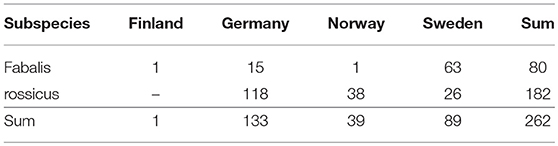
Table 1. Origin of the sampled individual.

The dataset contains 17 potentially explanatory variables (Table 2) and one response variable (fabalis = 1, rossicus = 0). Variable names are given in brackets in the text. For improved readability, the full variable names were replaced by single letter names (A-Q) in the output of some analyses (e.g., correlation matrix). The creation of new (composite) variables from existing ones (e.g., “Bill shape” = “Bill height” / “Culmen”) may seem appealing, but composite variables require special statistical considerations and thus, were largely avoided. The only exception was “Nail shape” = “Nail length” / “Nail width,” because the shape of the nail (clypea) on the bill was considered to be a strongly discriminating feature and recorded separately as a categorical variable (and thus unsuitable for most analyses used here). Potentially, this dataset allows for a huge amount of combinations of existing variables, with and without interactions. Because the aim of this study was the reduction of measurements and thus variables, rather than finding the best models, I chose to include only a few variable combinations at the final stages of model selection.

TABLE 2

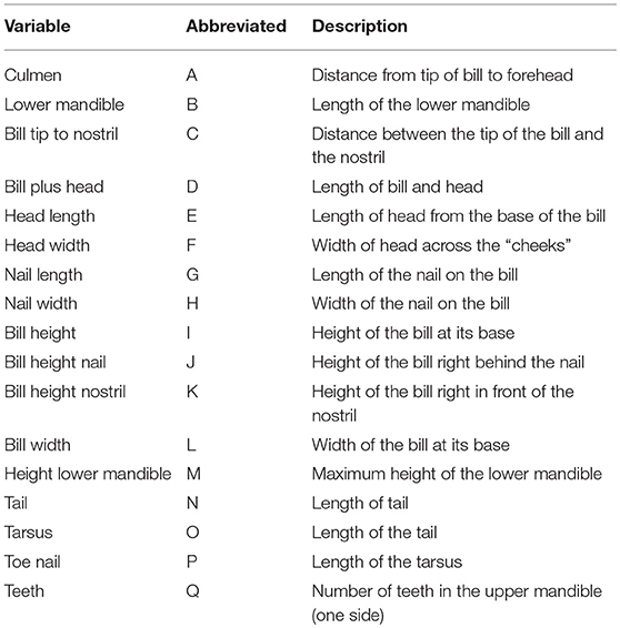
Table 2. Full and abbreviated variable names and a short description of their biological meaning.

Statistical Analysis

I screened the full set of potentially explanatory variables for subspecies determination by stepping through a number of statistical analyses on single, pairwise, and multiple variables (R functions in brackets, R script in Supplementary Material).

Individual Variables

After listing the basic statistics for individual variables, I visually inspected their frequency distributions (“histogram”) and incidence plots of their logistic models for subspecies discrimination (“glm, family = binomial”).

Pairwise Variables

First I plotted the observations against all variable pairs (“pairs”) and the correlation matrix (“cor” and “corrplot”). To exemplify the effect of the number of measured individuals, I also produced the correlation matrix analysis on a small (N = 20) random sub-set of the data. I then used partitioning of the observations on pairs of variables (“kmeans,” a simple form of cluster analysis) to visualize how well variable pairs could distinguish the subspecies.

Multiple Variables

I used discriminant analysis (“lda”) and AICc-based model selection of the logistic models (“aictab”) for multiple variable analyses. In the latter, I also included a selection of composite and multi variable models. Based on the results of the model selection process, I checked the quality of discriminant models for strongly reduced numbers of potentially explanatory variables (n = 5 and n = 2). Although Principle Component Analyses (PCAs) are popular for multivariate analyses and can produce visually appealing output, I chose to avoid PCA because they require pre-treatment of the input variables and their output is difficult to interpret [e.g., (41)]. In addition, PCAs aim to conserve rather than challenge existing variables, and thus, are less suitable for the purpose of this study.

All statistical analyses were made in R 3.4.4 x64 (42), with additional packages AICcmodavg (43), corrplot (44), lattice (45), lme4 (46), MASS (47), and Matrix (48), and supporting packages these depend on.

Animal Welfare

Based on personal experience from participating in most of the catching operations behind the dataset, I took times for taking the various measurements on a mock-up goose. I also estimated the times used for additional procedures of the most extensive protocol (Table 8). Times for catching and storage (in bags) were not included, because these vary dramatically with circumstances; many of which are beyond the control of the research team. All estimates assume the team to be well-trained and well-equipped for outdoor conditions. Estimates also assume that a dedicated staff member takes notes and other members take care of the logistics (e.g., photo-documentation and releasing the birds). Consequently, all estimates of handling times are conservative. In addition to handling times, I subjectively scored the level of invasiveness of each procedure on scale 1–10, with 10 being the highest level.

Results

The basic statistics (minimum, maximum, range, mean, standard deviation, and median) of all explanatory variables are presented in Table 3. The frequency distribution of a selection of four variables are shown in Figure 1. The upper two histograms (“Bill plus head” and “Bill height”) show unimodal distributions indicative of normal distribution across the entire sample. The lower two (“Height lower mandible” and “Teeth”) show bimodal distributions indicative of sub-grouping of the individuals based on these characteristics.

TABLE 3

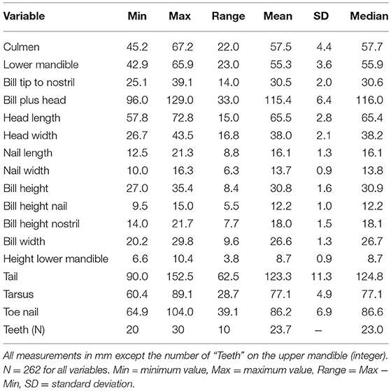
Table 3. Basic statistics.

FIGURE 1

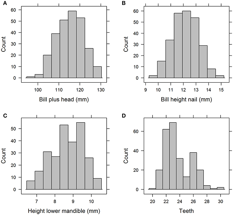
Figure 1. Histograms of a selection of the 17 variables, “Bill plus head” (A) and “Bill height nail” (B) with unimodal distribution vs “Height lower mandible” (C) and “Teeth” (D) with bimodal distribution.

Incidence curves for logistic models based on four individual variables are presented in Figure 2. Figure 2A shows a clear but not abrupt relationship between “Culmen” and subspecies (fabalis birds have longer culmen) in contrast to Figure 2B with virtually no effect of “Bill tip to nostril” (in fabalis and rossicus birds the distances are very similar). For “Height lower mandible” (Figure 2C), the curve dips fairly steep indicating a firm strong relationship with subspecies (rossicus birds have greater height = more pronounced “grin”). The variable “Teeth” (Figure 2D) reveals a very strong relationship with subspecies expressed as a sharp break at 24 teeth (fabalis birds have more teeth than rossicus). The model based on “Teeth” had by far the lowest AICc value (19) and thus, fitted the data best (Table 4). The “Height lower mandible” model came second (AICc = 136) while all other models had AICc > 189.

FIGURE 2

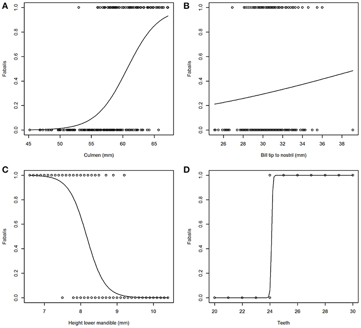
Figure 2. Incidence plots from a selection of logistic models for subspecies (rossicus = 0, fabalis = 1). Predicted responses go from poor in “Bill tip to nostril” (B) to distinct in “Teeth” (D). Variables “Culmen” (A) and “Height lower nmandible” (C) show intermediate, contra-directional responses.

TABLE 4

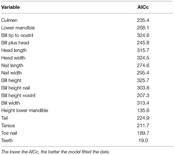
Table 4. AICc scores for all 17 single variable logistic models.

The Pairs plot (Figure 3) shows that observations are either aggregated along a trend line (indicative of correlation) or seemingly randomly dispersed across the plot area (indicative of absence of distinct grouping). In a plot with this many variables, the details of the distribution are not visible, though. For more detailed analysis, separate plots of variable pairs (“plot(x, y)”) are suggested (not included here, but described in the R scripts in Supplementary Material).

FIGURE 3

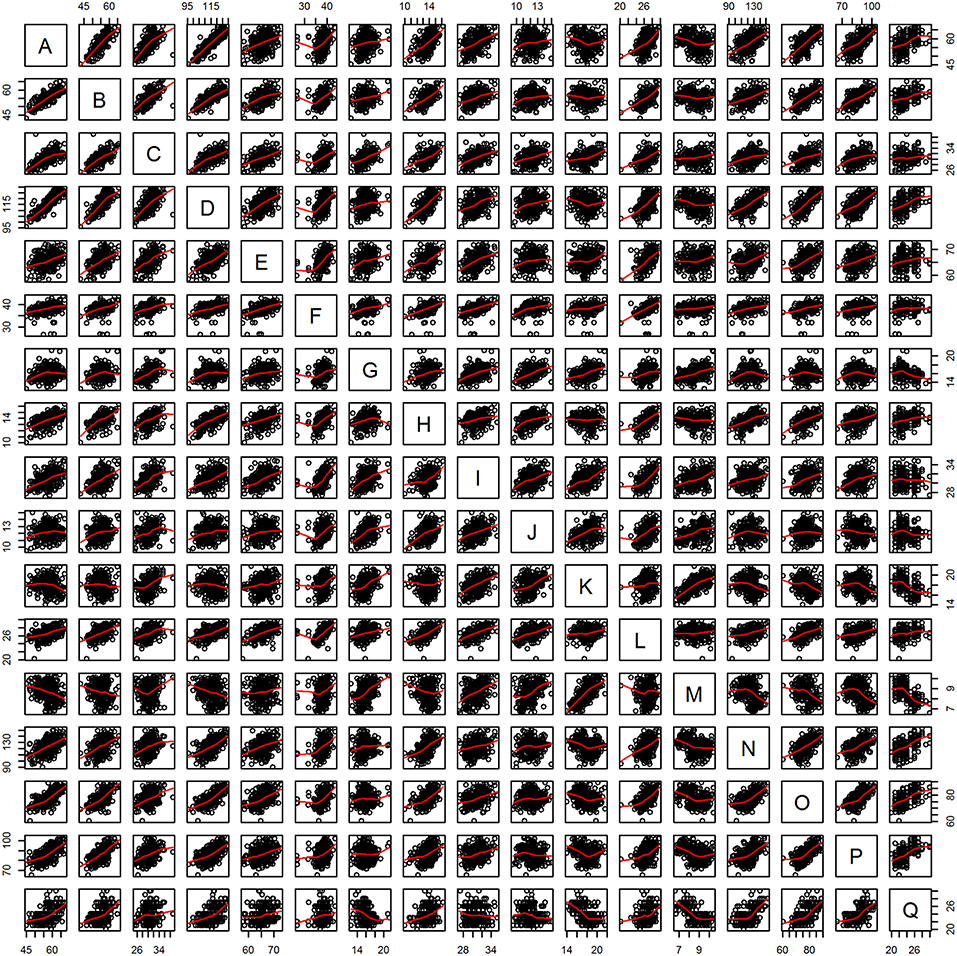
Figure 3. Panel plot of observations against pairs of variables. Trend lines in red. See Table 2 for variable name acronyms.

The correlation matrix (Figure 4) shows strong correlation between many of the variable pairs (high correlation coefficients and large dots). Most (85%) of the correlations were positive and 3.7% had >0.7 coefficients (8.1% > 0.6).

FIGURE 4

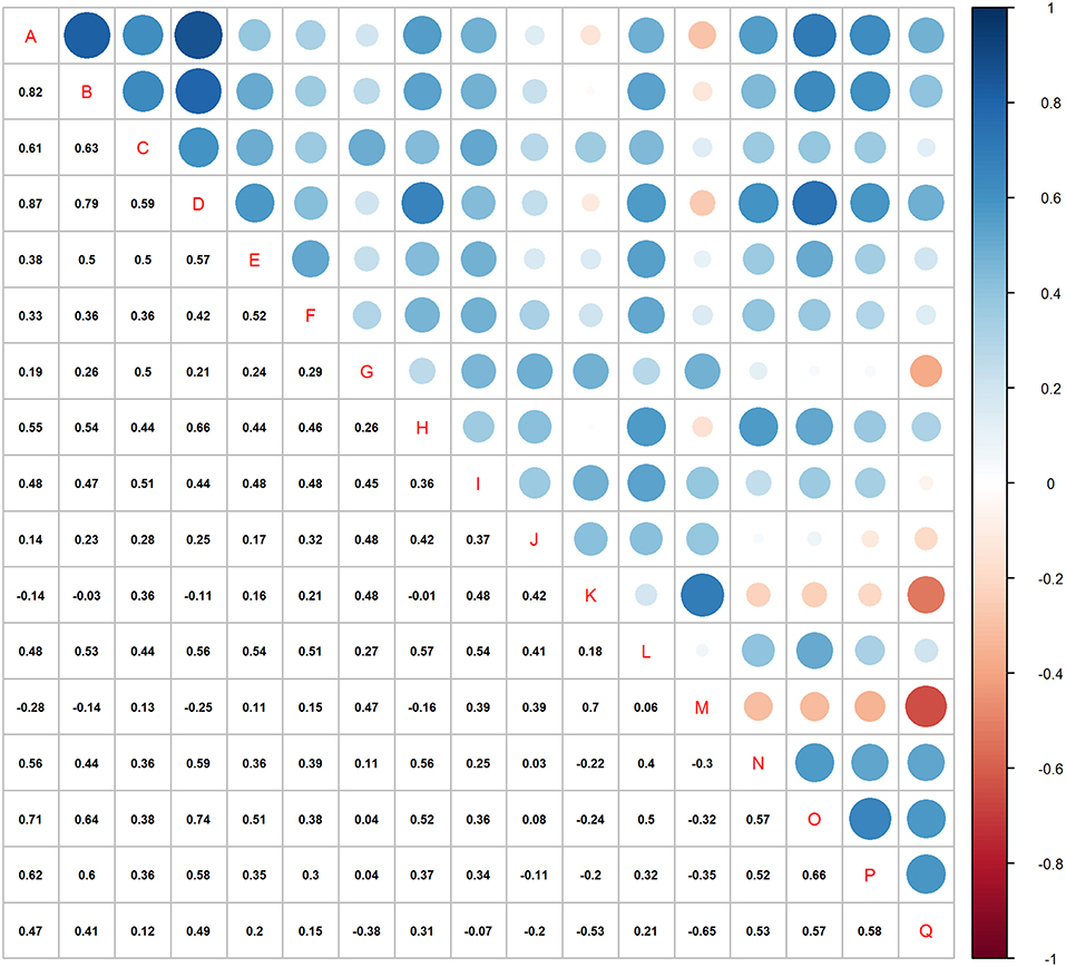
Figure 4. Correlation matrix for all 17 variables in the analyses. See Table 2 for variable name acronyms.

Two pairs of plots of the results of partitioning are presented here (Figure 5). For combination of “Culmen” and “Height lower mandible” the real and modeled distribution of the two subspecies are clearly different (upper panels). For the combination of “Teeth” and “Height lower mandible” the patterns of real and modeled distributions are almost identical (lower panels). The kmeans model based on the first pair of variables assigned only 30.5% of the individuals correctly while the second was accurate in 99.6% of the cases (Table 5).

FIGURE 5

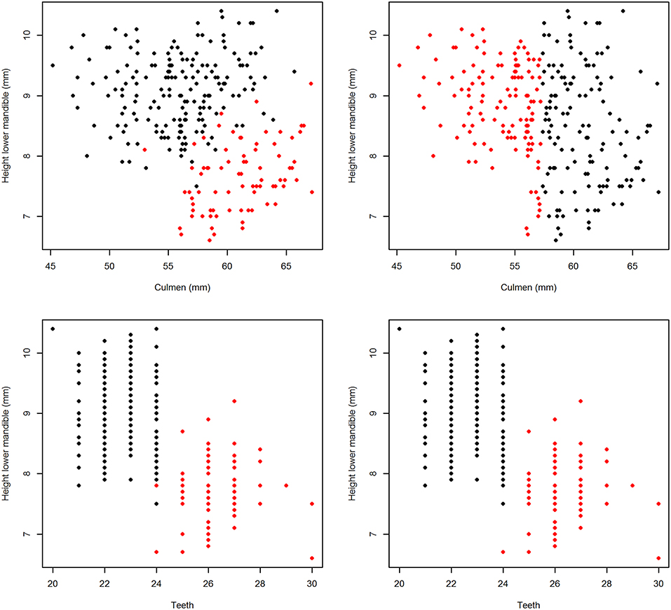
Figure 5. Plots of individual Bean Geese (fabalis = red, rossicus = black) on pairs of variables. (Left) original subspecies classification (ground truth). (Right) classification by the “kmeans” function.

TABLE 5

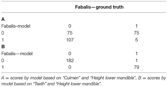
Table 5. Assignment of individuals to subspecies class by the kmeans models against the ground truth classification.

The fabalis and rossicus subspecies were well separated by the discriminant model based on all variables (Figure 6A). The linear discriminant coefficients (LDs) were highest for “Height lower mandible,” “Teeth” and “Nail length” (LD1 = −0.76, 0.62, and −0.36, respectively). Twelve (70%) of the variables had coefficients <0.1 and thus, contributed little to the discrimination process (Table 6). After removing all LD1 <0.1 variables, the remaining five variables still separated the subspecies nicely. Even with only “Height lower mandible” and “Teeth” included, the overlap between the subspecies was very small (Figure 6B). In the latter model, the coefficients were equally strong, but of opposite sign (−0.88 and 0.88, respectively).

FIGURE 6

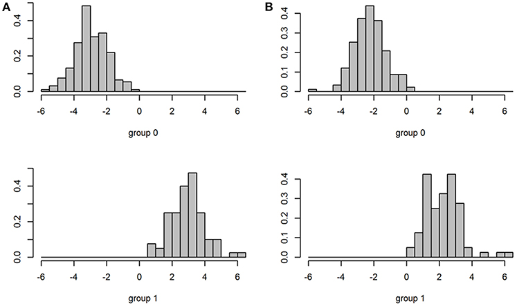
Figure 6. Plots of discrimination between subspecies (Group 0 = rossicus and Group 1 = fabalis) for models based on all 17 variables (A) and only two variables (B).

TABLE 6

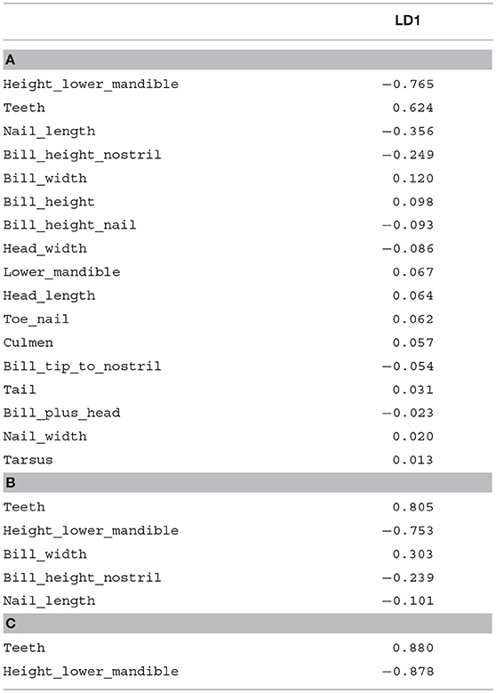
Table 6. Linear discriminant coefficients for model based on all 17 (A), five (B) and two variables (C).

In the formal AICc-based model selection process for the single variable logistic models (Table 7A), the “Teeth” variable virtually absorbed the entire AICcweight and thus, left very little credit for the other models. After adding four logistic models based on one composite variable (“Nail shape”) and three variable combinations, “Teeth & Height lower mandible” and “Teeth & Nail shape” proved to fit the data better than the “Teeth” variable alone (Table 7B). The difference between the top three models and the next was large (ΔAICc > 116).

TABLE 7

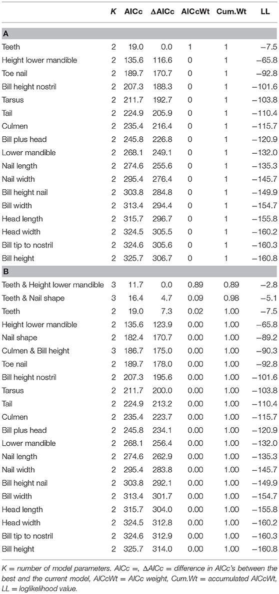
Table 7. AICc-based model selection for the 17 original single variable models (A) and the extended variable set (B).

The original 17 measurements took an estimated 209 s (3.5 min) to perform (Table 8). Based on the statistical analyses in this study, the number of measurements could have been reduced to only two (“Height lower mandible” and “Teeth”) without significant loss of discriminating power in subspecies identification. This reduction would have brought down the estimated time needed to take the necessary measurements to 37 s, 18% of the original time (Table 8).

TABLE 8

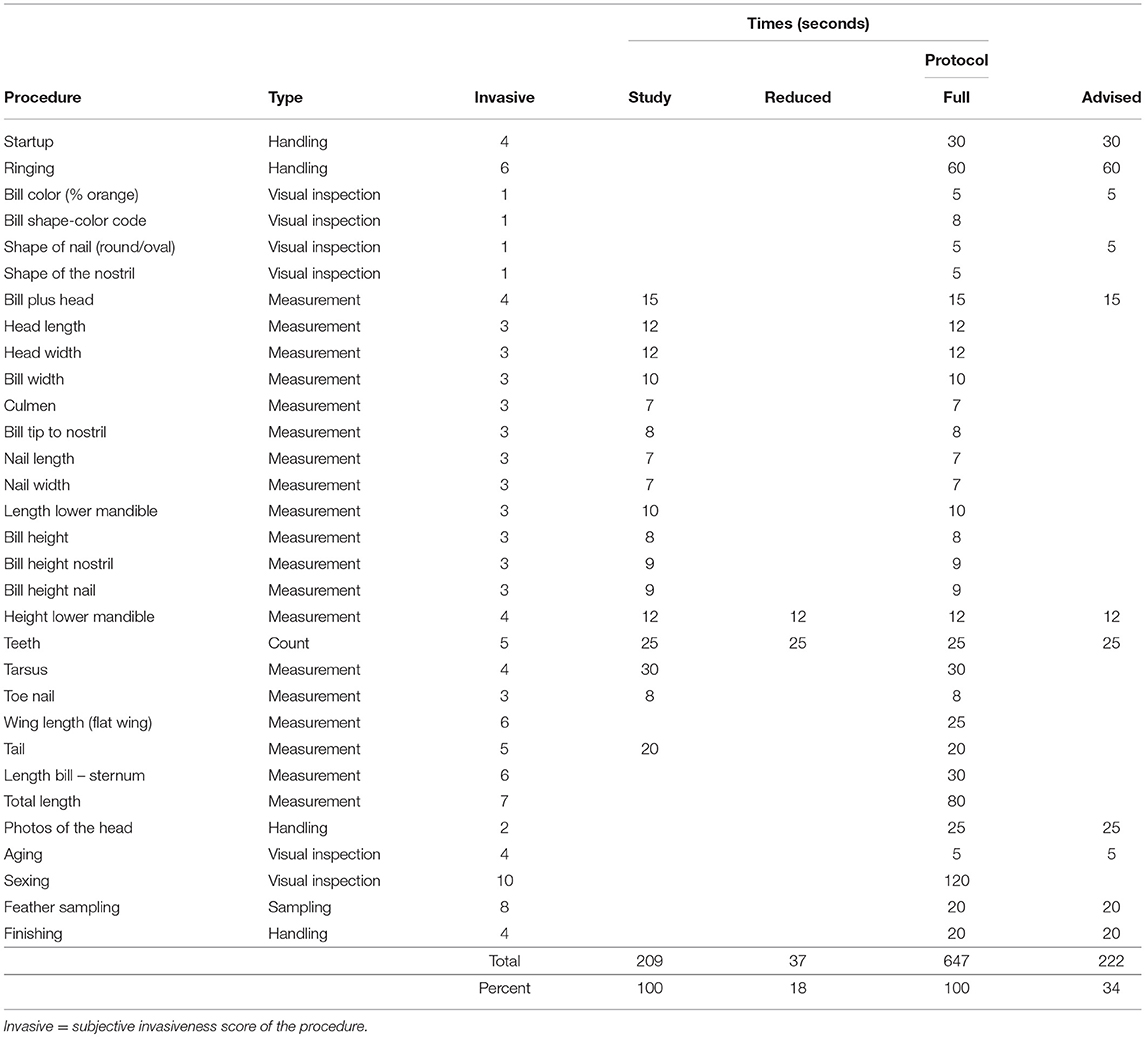
Table 8. Estimated duration (seconds) for actions in this study and in protocols for Bean Goose catching operations, with potential reductions based on the results of this study.

Across the full protocol of Bean Goose catching, overall time for handling an individual bird was estimated to 647 s (10.8 min). Based on the results of this study and the use of genetic sex markers, the completion of the protocol could be reduced by an estimated 66% (Table 8).

Discussion

In this dataset, two variables proved sufficient to distinguish between the two subspecies, the core objective of the data collection. The other 15 variables contributed virtually nothing and thus, should be considered redundant in this context. If these had been omitted from the measurement protocols, the 262 Bean Geese behind this study would have experienced an estimated reduction of 82% in time. Novel research is needed to reliably quantify the welfare impact of reduced measurement protocols, but the invasiveness scores of individual measurements (Table 8) suggest that some reductions are likely to have a greater impact than others.

The role for subspecies identification of the number of tomia (“teeth”) in the upper mandible and of the maximum height of the lower mandible (referred to as “grin” by field ornithologists) were commonly known before the sampling started [e.g., (49)]. The other variables were either proxies for size (fabalis is generally larger than rossicus, but so are males relative females) or indicators of complex features, e.g., “elongated bill” in fabalis vs. “short and distinct” bill in rossicus. Characterizing these shapes would often require the construction of composite variables (e.g., “Culmen”/“Bill height”). Composite variables often have complex error structures and thus, are statistically problematic (41). The perception of “jizz” (an overall, vague appearance/impression often used by birdwatchers) is difficult to frame with a simple set of measurement data. This example shows that the measurements taken failed to do so.

The dominance of “Teeth” and “Height lower mandible” was visible through the full chain of analyses. They were the only ones with a bimodal frequency distribution and showed the steepest curves in the incidence plots of the single variable logistic models (Figures 1, 2, respectively). Obviously, the use of logistic models is inappropriate for response variables with more than two classes. In these cases ANOVA or other classes of models should be used. The other components of the chain of analyses presented here would still be valid for non-binomial response variables.

Due to the high number of potentially explanatory variables, the “pairs” plot was not very informative (Figure 3), but a closer look at the plots for single pairs would have revealed more structure in the plots for the truly informative variables than the rest. The correlation matrix (Figure 4) showed that many variables were positively correlated. Strong positive correlations are indicative of redundant variables. Many of these correlated variables were associated with the size of the birds. In a PCA or Factor analysis, many of these variables had probably been bundled into a common PCA or Factor. In the light of this study, this would confirm that most of the bundled variables should have been omitted from the protocol. The use of plots and tables from “kmeans” showed that a combination of two variables could distinguish the subspecies adequately (Figure 5; Table 5).

For this dataset, the discriminant analysis separated the subspecies very well (Figure 6). The use of linear discriminant coefficients (Table 6) for the selection or omission of variables may be misleading if done in isolation (because the variables interact in the model). Here I used this technique as an integrated part of a screening scheme, which reduced most of the risks of sorting out important variables. With only two remaining variables, the subspecies separation was still good (Figure 6). In the final model selection step, the dominance of the “Teeth” variable stood out sharply among single variable models (Table 7). The effect of additional models confirmed this dominance and showed the potential of combining variables in model building. In this case, better models were constructed from the same duo of key variables and thus, did not motivate retaining other measurements. In cases when optimal models are important, more supporting variables (and thus more measurements) might be desirable, but the fringe benefit of keeping or introducing more variables needs to outweigh the negative impact on the birds exposed by the treatment.

From a statistical point of view, there are issues that could be brought up, especially if this variable screening strategy needs to be fully applicable to “problematic” datasets (e.g., datasets with diverse data quality levels or highly skewed variables), but this is beyond the scope of this study. My aim has been to demonstrate a simple, yet robust scheme for weeding out redundant variables and thus, omit unnecessary procedures in line with the Principles of the 3Rs. The supplemented R script can be used in this process.

This study was based on a single dataset of Bean Goose biometrics and further studies to demonstrate the potential of 3R implementation by reduced measuring are wanted. The levels of reduction in handling time shown in this example are highly encouraging and indicate significant 3R potential of reduced measurement protocols in wildlife research in general. Novel research is needed to reliably quantify the welfare impact of reduced measurement protocols, but the invasiveness scores of individual measurements (Table 8) suggest that some reductions are likely to have a greater impact than others. The search for redundant measurements will also raise 3R awareness in general, pointed out as a strong driver of improved animal welfare by Lindsjö et al. (10).

This study is also a good example of how existing data can be used to gain more knowledge; a case of combined Replacement and Reduction because no geese, only data, were handled for the purpose of this study. When applied in future studies on geese and other wildlife, the concluding recommendations will also lead to Refinement.

Similar schemes could also be developed for the Reduction of the numbers of geese and other animals used in wildlife research. Supplementary to the initial power analysis, the explanatory capacity of the collected data could be gradually evaluated and the inclusion of additional individuals halted when desired levels are reached.

Recommendations

I recommend a continuous process of challenging the necessity of measurements taken in wildlife research. Based on clear objectives and good knowledge of the research field, a minimized initial measurement protocol should be chosen. Once the set of measurement data grows (e.g., after each catching event), the dataset should be checked for weak or redundant measurements. Their place in the protocol should then be challenged. Arguments like “You never know how these data can be used in the future!” or “Colleague X may want to have these data.” might be tempting to apply, but do no longer fit into the modern world of research using live animals. If these arguments are truly relevant, the related measurements should be included in the initial protocol.

I also recommend that ECAEs, when applicable, demand a step-by-step motivation of each planned measurement and the inclusion of a reduction scheme similar to the one presented here. Finally, I recommend complementary studies on the reduction of potentially redundant measurements in research on other taxonomic groups and in-depth evaluations of how and to what extent reduced measuring actually improves the well-being of animals used in wildlife research.

A summary of this study and the full recommendation to omit several commonly applied measurements will be presented in Goose Bulletin, the official bulletin of the Goose Specialist Group of Wetlands International and IUCN. When implemented by the international goose research community, the proposed measurement reduction strategy could ease the life of hundreds of Bean Geese and thousands of other wild geese caught and handled by researchers annually.

Ethics Statement

Data had been collected by Dipl.Biol. Thomas Heinicke, Germany, during fully approved goose catching operations arranged by national research groups in Germany, Finland, Norway and Sweden 2007–2012. None of the measurements were taken for the purpose of this study, and the taking of the measurements was not subject to legal requirements of ECAE approval at the time and location of sampling.

Author Contributions

The author confirms being the sole contributor of this work and has approved it for publication.

Funding

This study was funded by a grant to the author from Petra Lundbergs Stiftelse¹.

Conflict of Interest Statement

The author declares that the research was conducted in the absence of any commercial or financial relationships that could be construed as a potential conflict of interest.

The reviewer EMW declared a shared affiliation, though no other collaboration, with the author to the handling Editor.

Acknowledgments

I am very grateful to Dipl.Biol. Thomas Heinicke, Humboldt-University, Berlin, Germany, for giving me access to this set of data. Three reviewers and the editor contributed to the quality of the final version of the manuscript.

Supplementary Material

The Supplementary Material for this article can be found online at: https://www.frontiersin.org/articles/10.3389/fvets.2019.00195/full#supplementary-material

Footnote

1. ^http://www.petralundbergsstiftelse.se/

References

1. Rollin BE. The regulation of animal research and the emergence of animal ethics: a conceptual history. Theor Med Bioeth. (2006) 27:285–304. doi: 10.1007/s11017-006-9007-8

PubMed Abstract | CrossRef Full Text | Google Scholar

2. EU. Directive 2010/63/EU of the European Parliament and of the Council of 22 September 2010 on the Protection of Animals Used for Scientific Purposes. (2010). Available online at: http://eur-lex.europa.eu/LexUriServ/LexUriServ.do?uri=OJ:L:2010:276:0033:0079:EN:PDF (accessed February 08, 2018).

Google Scholar

3. Jordbruksverket. Föreskrifter och allmänna råd om försöksdjur. SJVFS 2017:40. Jönköping: Jordbruksverket (2017).

Google Scholar

4. Russell WMS, Burch RL. The Principles of Humane Experimental Technique. London: Methuen (1959).

Google Scholar

5. Forni M. Laboratory animal science: a resource to improve the quality of science. Vet Res Comm. (2007) 31:43–7. doi: 10.1007/s11259-007-0096-2

PubMed Abstract | CrossRef Full Text | Google Scholar

6. Fenwick N, Danielson P, Griffin G. Survey of Canadian animal-based researcher's views on the three Rs: replacement, reduction and refinement. PLoS ONE. (2011) 6:e22478. doi: 10.1371/journal.pone.0022478

CrossRef Full Text | Google Scholar

7. Törnqvist E, Annas A, Granath B, Jalkesten E, Cotgreave I, Öberg M. Strategic focus on 3R principles reveals major reductions in the use of animals in pharmaceutical toxicity testing. PLoS ONE. (2014) 9:e101638. doi: 10.1371/journal.pone.0101638

PubMed Abstract | CrossRef Full Text | Google Scholar

8. Blattner CE. 3R for farmed animals – a legal argument for consistency. Global J Ani Law. (2014). p. 26. Retrieved from: https://ojs.abo.fi/ojs/index.php/gjal/article/view/1303

Google Scholar

9. Lundmark F, Berg C, Röcklinsberg H. Regelverk för djurskydd—vad vill man uppnå? Sv Veterinärtidn. (2014) 66:11–7. doi: 10.1007/s10806-014-9512-0

CrossRef Full Text | Google Scholar

10. Lindsjö J, Fahlman Å, Törnqvist E. Animal welfare from mouse to moose—implementing the principles of the 3Rs in wildlife research. J Wildl Dis. (2016) 52:65–77. doi: 10.7589/52.2S.S65

PubMed Abstract | CrossRef Full Text | Google Scholar

11. Ainley MG. The contribution of the amateur to North American ornithology: a historical perspective. Living Bird. (1979) 18:161–77.

Google Scholar

12. Mayfield HF. The amateur in ornithology. Auk. (1979) 96:168–71.

Google Scholar

13. Mayfield HF. The amateur: finding a niche in ornithology. Nebra Bird Rev. (1991) 416:39–41.

Google Scholar

14. Fox AD, Madsen J. Behavioural and distributional effects of hunting disturbance on waterbirds in Europe: implications for refuge design. J Appl Ecol. (1997) 34:1–13. doi: 10.2307/2404842

CrossRef Full Text | Google Scholar

15. Jordbruksverket. Användning av försöksdjur i Sverige Under 2016. Rapport 2018-03-07. Jönköping: Jordbruksverket (2018).

Google Scholar

16. Ringmärkningscentralen. Antal ringmärkta och återfunna fåglar 2017. (2018). Stockholm. Available online at: http://www.nrm.se/forskningochsamlingar/miljoforskningochovervakning/ringmarkningscentralen/ringmarkningochaterfynd.763.html (accessed February 15, 2018).

Google Scholar

17. Landys-Ciannelli MM, Ramenofsky M, Piersma T, Jukema J, Wingfield JC. Baseline and stress-induced plasma corticosterone during long-distance migration in the Bar-Tailed Godwit, Limosa lapponica. Physiol Bioch Zool. (2002) 75:101–10. doi: 10.1086/338285

PubMed Abstract | CrossRef Full Text | Google Scholar

18. Romero LM, Romero RC. Corticosterone responses in wild birds: the importance of rapid initial sampling. Condor. (2002) 104:129–35. doi: 10.1650/0010-5422(2002)104[0129:CRIWBT]2.0.CO;2

CrossRef Full Text | Google Scholar

19. Weimerskirch H, Shaffer SA, Mabille G, Martin J, Boutard O, Rouanet JL. Heart rate and energy expenditure of incubating wandering albatrosses: basal levels, natural variation, and the effects of human disturbance. J Exp Biol. (2002) 205:475–83. Available online at: http://jeb.biologists.org/content/205/4/475

PubMed Abstract | Google Scholar

20. Ankney CD. An embarrassment of riches: too many geese. J Wildl Manag. (1996) 60:217–23. doi: 10.2307/3802219

CrossRef Full Text | Google Scholar

21. Fox AD, Ebbinge BS, Mitchell C, Heinicke T, Aarvak T, Colhoun K, et al. Current estimates of goose population sizes in western Europe, a gap analysis and an assessment of trends. Ornis Svec. (2010) 20:115–27. Available online at: http://birdlife.se/wp-content/uploads/ornis_svecica/cms_20-s1_Vol%2020(3-4),%20115-127,%20Fox%20et%20al.%20Review.pdf

Google Scholar

22. IUCN. The IUCN Red List of Threatened Species. Version 2017-1 (2017). Available online at: http://www.iucnredlist.org/ (accessed July 09, 2017).

PubMed Abstract | Google Scholar

23. Delacour J. Taxonomic notes on the bean goose Anser fabalis Lath. Ardea. (1951) 39:135–42.

Google Scholar

24. Burgers J, Smit JJ, van der Voet H. Origins and systematics of two types of the Bean Goose Anser fabalis (Latham, 1787) wintering in The Netherlands. Ardea. (1991) 79:307–16.

Google Scholar

25. Sangster G, Oreel GJ. Progress in taxonomy of Taiga and Tundra Bean Geese. Dutch Birding. (1996) 18:310–6.

Google Scholar

26. van den Bergh L. Geografische variatie bij Ganzen. Deel 3. De West-Siberische Taigagans of Johansens Gans Anser fabalis johanseni. Vogeljaar. (2003) 51:58–64. Available online at: http://natuurtijdschriften.nl/search?identifier=544861

Google Scholar

27. Koffijberg K, Hustings F, de Jong A, Hornman M, van Winden E. Recente ontwikkelingen in het voorkomen van Taigarietganzen in Nederland. Limosa. (2011) 84:117–31. Available online at: http://limosa.nou.nu/nou_login.php?nr=4182

Google Scholar

28. Ruokonen M, Litvin K, Aarvak T. Taxonomy of the bean goose - pink-footed goose. Mol Phylogen Evol. (2008) 48:554–62. doi: 10.1016/j.ympev.2008.04.038

PubMed Abstract | CrossRef Full Text | Google Scholar

29. Heinicke T. Status of the Bean Goose Anser fabalis wintering in central Asia. Wildfowl. (2009) 59:77–99. Available online at: https://wildfowl.wwt.org.uk/index.php/wildfowl/article/view/1215

Google Scholar

30. Marjakangas A, Alhainen M, Fox AD, Heinicke T, Madsen J, Nilsson L, et al. International Single Species Action Plan for the Conservation of the Taiga Bean Goose Anser fabalis fabalis. Bonn: AEWA Technical Service No. XX (2015).

Google Scholar

31. Hirschfeld A, Heyd A. Mortality of migratory birds caused by hunting in Europe: bag statistics and proposals for the conservation of birds and animal welfare. Ber zum Vogelsch. (2005) 42:47–74.

Google Scholar

32. Hake M, Månsson J, Wiberg A. A working model for preventing crop damage caused by increasing goose populations in Sweden. Ornis Svec. (2010) 20:225–33. Available online at: http://birdlife.se/wp-content/uploads/ornis_svecica/cms_20-s1_Vol%2020(3-4),%20225-233,%20Hake%20et%20al%20Working%20model.pdf

Google Scholar

33. Fox AD, Elmberg J, Tombre IM, Hessel R. Agriculture and herbivorous waterfowl: a review of the scientific basis for improved management. Biol Rev. (2016) 92:854–77. doi: 10.1111/brv.12258

PubMed Abstract | CrossRef Full Text | Google Scholar

34. Madsen J, Guillemain M, Nagy S, Defos du Rau P, Mondain-Monval J-Y, Griffin C, et al. Towards Sustainable Management of Huntable Migratory Waterbirds in Europe: A Report by the Waterbird Harvest Specialist Group of Wetlands International. (2015). The Netherlands: Wetlands International. Available online at: https://www.wetlands.org/publications/towards-sustainable-management-of-huntable-migratory-waterbirds-in-europe/ (accessed May 03, 2017).

Google Scholar

35. Nilsson L, de Jong A, Heinicke T, Sjöberg K. Satellite tracking of Bean Geese Anser fabalis fabalis and A. f. rossicus from spring staging areas in Northern Sweden to breeding and moulting areas. Ornis Svec. (2010) 20:184–9. Available online at: http://birdlife.se/wp-content/uploads/ornis_svecica/cms_20-s1_Vol%2020(3-4),%20184-189,%20Nilsson%20satellite.pdf

Google Scholar

36. Fox AD, Hobson KA, de Jong A, Kardynal KJ, Koehler G, Heinicke T. Flyway population delineation in Taiga Bean Geese Anser fabalis fabalis revealed by multi-element feather stable isotope analysis. Ibis. (2016) 159:66–75. doi: 10.1111/ibi.12417

CrossRef Full Text | Google Scholar

37. Mitchell C, Griffin L, Maciver A, Minshull B, Makan N. Use of GPS tags to describe the home ranges, migration routes, stop-over locations and breeding area of Taiga Bean Geese Anser fabalis fabalis wintering in central Scotland. Bird Study. (2016) 63:437–46. doi: 10.1080/00063657.2016.1236779

CrossRef Full Text | Google Scholar

38. Heinicke T, Mooij J, Steudtner J. Zur Bestimmung von Saatgans (Anser f. fabalis, A f rossicus) und Kurzschnabelgans (Anser brachyrhynchus) und deren Auftreten in Ostdeutschland. Mitt Ver Sächs Ornithol. (2005) 9:533–53.

Google Scholar

39. Heinicke T. Tundra bean goose Anser fabalis rossicus during spring migration in northern Sweden—rare visitor or regular passage migrant? Ornis Svec. (2010) 20:174–83. Available online at: http://birdlife.se/wp-content/uploads/ornis_svecica/cms_20-s1_Vol%2020(3-4),%20174-183,%20Heinicke%20Tundra%20Bean.pdf

PubMed Abstract | Google Scholar

40. Dzubin A, Cooch E. Measurements of Geese: General Field Methods. Sacramento, CA: California Waterfowl Association (1992).

Google Scholar

41. Crawley MJ. The R Book. Chichester: Wiley and Sons (2007). doi: 10.1002/9780470515075

CrossRef Full Text | Google Scholar

42. R Core Team (2018). R: A Language and Environment for Statistical Computing. Vienna: R Foundation for Statistical Computing. Available online at: https://www.R-project.org/

PubMed Abstract | Google Scholar

43. Mazerolle MJ. AICcmodavg: Model Selection and Multimodel Inference Based on (Q)AIC(c). R Package Version 2.1-1 (2017). Available online at: https://cran.r-project.org/package=AICcmodavg

Google Scholar

44. Wei T, Simko V. R package “corrplot”: Visualization of a Correlation Matrix. (Version 0.84) (2017). Available online at: https://github.com/taiyun/corrplot (accessed May 04, 2018).

Google Scholar

45. Sarkar D. Lattice: Multivariate Data Visualization With R. New York, NY: Springer (2008).

Google Scholar

46. Bates D, Maechler M, Bolker B, Walker S. Fitting linear mixed-effects models using lme4. J Stat Softw. (2015) 67:1–48. doi: 10.18637/jss.v067.i01

CrossRef Full Text | Google Scholar

47. Venables WN, Ripley BD. Modern Applied Statistics With S, 4th edn. New York, NY: Springer (2002).

Google Scholar

48. Bates D, Maechler M. Matrix: Sparse and Dense Matrix Classes and Methods. R package version 1.2-14 (2018). Available online at: https://CRAN.R-project.org/package=Matrix (accessed May 09, 2018).

Google Scholar

49. Cramp S (ed.). Handbook of the Birds of Europe, the Middle East and North Africa. Oxford: Oxford University Press (1977).

Google Scholar