LVAC: Learned volumetric attribute compression for point clouds using coordinate based networks

1 Introduction

Upon the recent success of implicit networks, a. k.a. coordinate-based networks (CBNs), in representing a variety of signals such as neural radiance fields (Mildenhall et al., 2020; Yu A. et al., 2021; Barron et al., 2021; Hedman et al., 2021; Knodt et al., 2021; Srinivasan et al., 2021; Zhang et al., 2021), point clouds (Fujiwara and Hashimoto, 2020), meshes (Park et al., 2019a; Mescheder et al., 2019; Sitzmann et al., 2020; Martel et al., 2021; Takikawa et al., 2021), and images (Martel et al., 2021), an end-to-end compression framework for representations using CBNs has become inevitably necessary. Motivated by this, we propose the first end-to-end learned compression framework for volumetric functions represented by CBNs with a focus on point cloud attributes as other representations lack baselines to compare with. We call our method Learned Volumetric Attribute Compression (LVAC). Point clouds are a fundamental data type underlying 3D sampling and hence play a critical role in applications such as mapping and navigation, virtual and augmented reality, telepresence, and cultural heritage preservation, which rely on sampled 3D data (Mekuria et al., 2017; Park et al., 2019a; Pierdicca et al., 2020; Sun et al., 2020). Given the volume of data in such applications, compression is important for both storage and communication. Indeed, standards for point cloud compression are underway in both MPEG and JPEG (Schwarz et al., 2019; Jang et al., 2019; Graziosi et al., 2020; 3DG, 2020a).

3D point clouds, such as those shown in Figure 1, each consist of a set of points {(x_i, y_i)}, where x_i is the 3D position of the ith point and y_i is a vector of attributes associated with the point. Attributes typically include color components, e.g., RGB, but may alternatively include reflectance, normals, transparency, density, spherical harmonics, and so forth. Commonly (Zhang et al., 2014; Cohen et al., 2016; de Queiroz and Chou, 2016; Thanou et al., 2016; de Queiroz and Chou, 2017; Pavez et al., 2018; Schwarz et al., 2019; Chou et al., 2020; Krivokuća et al., 2020), point cloud compression is broken into two steps: compression of the point cloud positions, called the geometry, and compression of the point cloud attributes. As illustrated in Figure 2, once the decoder decodes the geometry (possibly with loss), the encoder encodes the attributes conditioned on the decoded geometry. In this work, we focus on this second step, namely attribute compression conditioned on the decoded geometry, assuming geometry compression (such as Krivokuća et al., 2020; Tang et al., 2020) in the first step. It is important to note that this conditioning is crucial in achieving good attribute compression. This will become one of the themes of this paper.

FIGURE 1

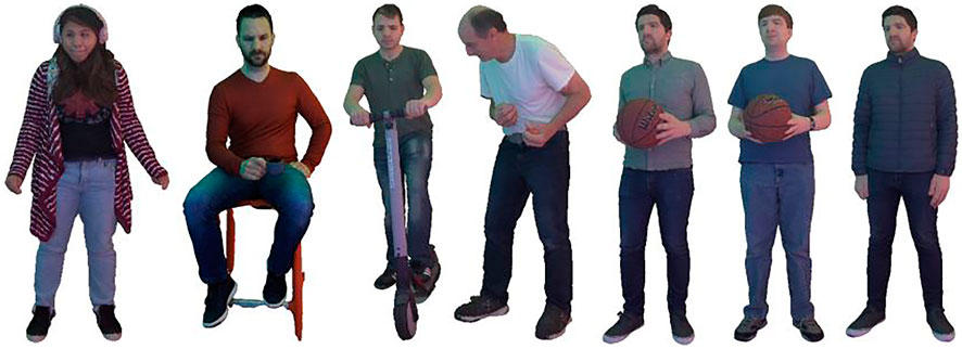
FIGURE 1. Point clouds rock, chair, scooter, juggling, basketball1, basketball2, and jacket.

FIGURE 2

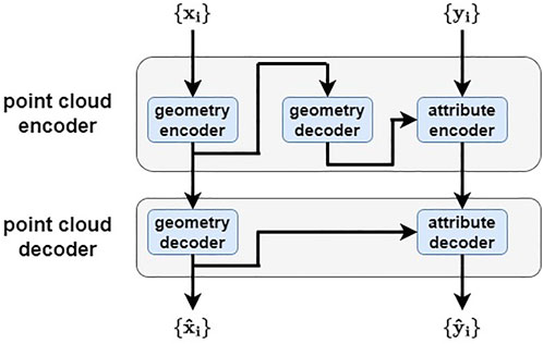
FIGURE 2. Point cloud codec: a geometry encoder and decoder, and an attribute encoder and decoder conditioned on the decoded geometry.

Following successful application of neural networks in image compression (Ballé et al., 2016; Toderici et al., 2016; Ballé et al., 2017; Toderici et al., 2017; Ballé, 2018; Ballé et al., 2018; Minnen et al., 2018; Balle et al., 2020; Mentzer et al., 2020; Hu et al., 2021), neural networks have been used successfully for point cloud geometry compression, demonstrating significant gains over traditional techniques (Yan et al., 2019; Quach et al., 2019; Guarda et al., 2019a,b; Guarda et al., 2020; Tang et al., 2020; Quach et al., 2020b). However, the same cannot be said for point cloud attribute compression. To our knowledge, our work is among the first to use neural networks for point cloud attribute compression. Previous attempts have been hindered by the inability to properly condition the attribute compression on the decoded geometry, thus leading to poor results. In our work, we show that proper conditioning improves attribute compression performance by over 30% reduction in the BD-rate. This results in a gain of 2–4 dB in the reconstructed colors over region-adaptive linear transform (RAHT) coding (de Queiroz and Chou, 2016), which is used in the “geometry-based” point cloud compression standard of MPEG G-PCC. Additionally, we compare our method with a recent learned framework Deep-PCAC (Sheng et al., 2021), which is not volumetric, and outperform it by 3–5 dB.

Although learned image compression systems have been based on convolutional neural networks (CNNs), in this work we use what have come to be called coordinate based networks (CBNs), also called implicit networks. A CBN is a network, such as a multilayer perceptron (MLP), whose inputs include the coordinates of the spatial domain of interest, e.g., $\mathbf{x}\in {\mathbb{R}}^3$. We use lightweight MLPs with one hidden layer as CBNs. Keeping the CBNs relatively small provides (1) efficient training/inference and (2) negligible overhead for representing the CBN. A CBN can directly represent a nonlinear function of the spatial coordinates x, possibly indexed with a latent or feature vector z, as y = f_θ(x) or y = f_θ(x; z). CBNs have recently come to the fore in accurately representing geometry and spatial phenomena such as radiance fields. However, while there has been an explosion of work using CBNs for representing specific objects and scenes (Park et al., 2019a; Mescheder et al., 2019; Mildenhall et al., 2020; Sitzmann et al., 2020; Yu A. et al., 2021; Barron et al., 2021; Hedman et al., 2021; Knodt et al., 2021; Martel et al., 2021; Srinivasan et al., 2021; Takikawa et al., 2021; Zhang et al., 2021), none of that work focuses on compressing those representations. (Two exceptions may be (Bird et al., 2021; Isik, 2021), which simply apply model compression to the CBNs.). Good lossy compression is nontrivial, and must make the optimal trade-off between the fidelity of the reconstruction and the number of bits used in its binary representation. We show that naïve scalar quantization and entropy coding of the parameters θ and/or latent vectors z lead to very poor results, and that superior results can be achieved by proper orthonormalization prior to uniform scalar quantization. In addition, for the best rate-distortion performance, the entropy model and CBN must be jointly trained to minimize a loss function that penalizes not only large distortion (or error) but large bit rate as well. We achieve this via a rate-distortion Lagrangian loss. Our main contributions include the following:

• We are the first to compress volumetric functions modeled by local coordinate based networks, by performing an end-to-end optimization of a rate-distortion Lagrangian loss function, thereby offering scalable, high fidelity reconstructions even at low bit rates. We show that naïve uniform scalar quantization and entropy coding lead to poor results.

• We apply our framework to compress point cloud attributes. (It is applicable to other signals as well such as neural radiance fields, meshes, and images.) Hence, we are the first to compress point cloud attributes using CBNs. Our solution allows the network to interpolate the reconstructed attributes continuously across space, and offers a 2–5 dB improvement over our learned baseline Deep-PCAC (Sheng et al., 2021) and a 2–4 dB improvement over our linear baseline, RAHT (de Queiroz and Chou, 2016) with adaptive Run-Length Golomb-Rice (RLGR) entropy coding—the transform in the latest MPEG G-PCC standard.

• We show formulas for orthonormalizing the coefficients to achieve over a 30% reduction in bit rate. Note that appropriate orthonormalization is an essential (and nontrivial) component of all compression pipelines.

Section 2 provides a brief overview of our Learned Volumetric Attribute Compression (LVAC) framework without going into the details, Section 3 covers related work, Section 4 details our framework, Section 5 reports experimental results, and Section 6 discusses and concludes. We provide a list of notations used in the paper in Supplementary Table S1.

2 Overview of the framework

The goal of this work is to develop a volumetric point cloud attribute compression framework that uses the decoded geometry as side information. Unlike standard linear transform coding approaches such as RAHT, our approach performs non-linear interpolation through the learned volumetric functions modeled by neural networks.

Our approach is summarized in Figure 3, where we jointly train 1) some transform coefficients V for the point cloud blocks, 2) quantizer stepsizes, 3) an entropy coder, and 4) a CBN via backpropagation through a Lagrangian loss function D + λR. Here D is the distortion between the reconstructed attributes and the true attributes (color attributes in this work), and R is the estimated entropy of the quantized transform coefficients $\widehat{\mathbf{V}}$, computed by our neural entropy model, which is a differentiable proxy for the “non-differentiable” entropy coder. The quantized transform coefficients $\widehat{\mathbf{V}}$ are inverse transformed via a linear synthesis matrix T_s as in standard transform coding frameworks. Notice, however, that we omit the usual analysis transform prior to quantization. This is because we directly learn the transform coefficients V through optimization for each point cloud ¹. These learned transform coefficients V are then quantized and synthesized into latent vectors $\widehat{\mathbf{Z}}=[{\widehat{\mathbf{z}}}_{\mathbf{n}}]$ as shown in the figure. While the synthesized latent vector ${\widehat{\mathbf{z}}}_{\mathbf{n}}$ for the block that a query point resides in could be output as the reconstructed attributes for that point, we take one step further and introduce a non-linear operation: We feed a small neural network, namely a CBN, with the synthesized latent vector and the 3D location of the query point x. This network outputs the reconstructed attributes, which are used in our distortion calculation. Finally, our Lagrangian loss is calculated with the estimated rate and the distortion, and this loss is backpropagated through all the blocks in Figure 3. As we will explain in Section 4, the synthesis matrix T_s is not learned. However, it is a fixed function of the geometry, as in RAHT. In fact, our synthesis transform can be regarded as the RAHT synthesis transform operating on latent vectors rather than attributes. Thus, we compress our latent vectors conditioned on the geometry as side information. All components besides the synthesis matrix such as the transform coefficients V, the quantization stepsizes, the entropy model, and the CBN are jointly trained through the Lagrangian loss function that optimizes both the reconstructions and the bitrate.

FIGURE 3

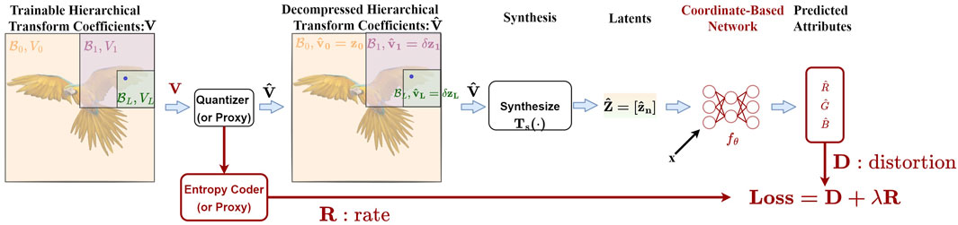
FIGURE 3. Querying attributes at position $\mathbf{x}\in {\mathbb{R}}^3$. The block ${\mathcal{B}}_{\mathbf{n}(\mathbf{x})}$ at target level L in which x is located is identified by traversing a binary space partition tree. The “learnable” transform coefficients V are first quantized by rounding to obtain $\widehat{\mathbf{V}}=\lfloor \mathbf{V}\rceil$, and then the latent vectors are reconstructed as $\widehat{\mathbf{Z}}={\mathbf{T}}_s\widehat{\mathbf{V}}$. V is optimized by back-propagating D (θ, Z)+ λR (θ, Z) through all the components in the figure. The pipeline uses differentiable proxies for the quantizer and entropy coder. In Figure 4, we give more details on the quantization and the orthonormalization steps, which are omitted in this figure for simplicity.

As we dive into the details of Figure 3 in the following sections, we try to address the following challenges:

• It is essential to make sure that the coefficients are orthonormalized prior to quantization. Otherwise, the quantization error would accumulate across different channels. To achieve this, we need to introduce orthonormalization and de-orthonormalization steps before and after the quantization.

• Both quantization and entropy coding are non-differentiable operations. Thus, we need to utilize diffentiable proxies to perform backpropagation during training.

3 Related work

3.1 Learned image compression

Using neural networks for good compression is non-trivial. Simply truncating the latent vectors of an existing representation to a certain number of bits is likely to fail, if only because small quantization errors in the latents may easily map into large quantization errors in their reconstructions. Moreover, the entropy of the quantized latents is a more important determiner of the bit rate than the total number of coefficients in the latent vectors or the number of bits in their binary representation. Early work on learned image compression could barely exceed the rate-distortion performance of JPEG on low-quality 32 × 32 thumbnails (Toderici et al., 2016). However, over the years the rate-distortion performance has consistently improved (Ballé et al., 2016; Ballé et al., 2017; Toderici et al., 2017; Ballé, 2018; Ballé et al., 2018; Minnen et al., 2018; Balle et al., 2020; Cheng et al., 2020; Hu et al., 2021) to the point where the best learned image codecs outperform the latest video standard (VVC) in PSNR, albeit at much greater complexity (Guo et al., 2021), and greatly outperform conventional image codecs (by over 2× reduction in bit rate) at the same perceptual distortion (Mentzer et al., 2020). Essentially all current competitive learned image codecs are versions of nonlinear transform coding (Balle et al., 2020), in which the bottleneck latents in an auto-encoder are uniformly scalar quantized and entropy coded, for transmission to a decoder. The decoder uses a convolutional neural network as a synthesis transform. The codec parameters θ are trained end-to-end through a differentiable proxy for the quantizer, often modeled as additive uniform noise. The loss function is a Lagragian L(θ) = D(θ) + λR(θ), where D(θ) and R(θ) are the expected distortion and bit rate. In this work, we use similar proxies for uniform scalar quantization and entropy coding as used for the learned image compression and train our representation using a similar loss function.

3.2 Coordinate based networks

Early work that used coordinate based networks (Park et al., 2019a; Mescheder et al., 2019; Sitzmann et al., 2020), exemplified by DeepSDF (Park et al., 2019b), focused on representing geometry implicitly, e.g., as the c-level set $\{\mathbf{x}:c=f_{\theta }(\mathbf{x};\mathbf{z})\}\subset {\mathbb{R}}^3$ of a function $f_{\theta }:{\mathbb{R}}^3\times {\mathbb{R}}^C\to \mathbb{R}$ modeled by a neural network, where $\mathbf{z}\in {\mathbb{R}}^C$ is a global latent vector. As a result such networks were called “implicit” networks. Much of this work focused on auto-decoder architectures, in which the latent vector z was determined for each instance by back propagation through the loss function. The loss function L (θ, z) measured a pointwise error between samples f_θ(x_i; z) of the network and samples f (x_i) of a ground truth function, such as the signed distance function (SDF).

Later work that used CBNs, exemplified by NeRF (Mildenhall et al., 2020; Barron et al., 2021), used the networks to model not SDFs but rather other, vector-valued, volumetric functions, including color, density, normals, BRDF parameters, and specular features (Yu A. et al., 2021; Hedman et al., 2021; Knodt et al., 2021; Srinivasan et al., 2021; Zhang et al., 2021). Since these networks were no longer used to represent solutions implicitly, their name started to shift to “coordinate-based” networks, e.g., (Tancik et al., 2021). An important innovation from this cohort was measuring the loss L(θ) not pointwise between samples of f_θ and some ground truth volumetric function f, but rather between volumetric renderings (to images) of f_θ and f, the latter renderings being ground truth images.

Mildenhall et al. (2020) focused on training the CBN f_θ(x) to globally represent a single scene, without benefit of a latent vector z. However, subsequent work shifted towards using the CBN with different latent vectors for different objects (Stelzner et al., 2021; Yu H.-X. et al., 2021; Kundu et al., 2022a,b) or different regions (i.e., blocks or tiles) in the scene (Chen et al., 2021; DeVries et al., 2021; Martel et al., 2021; Mehta et al., 2021; Reiser et al., 2021; Takikawa et al., 2021; Rematas et al., 2022; Tancik et al., 2022; Turki et al., 2022). Partitioning the scene into blocks, and using a CBN with a different latent vector in each block, simultaneously achieves faster rendering (Reiser et al., 2021; Takikawa et al., 2021), higher resolution (Chen et al., 2021; Martel et al., 2021; Mehta et al., 2021), and scalability to scenes of unbounded size (DeVries et al., 2021; Rematas et al., 2022; Tancik et al., 2022; Turki et al., 2022). However, this puts much of the burden of the representation on the local latent vectors, rather than on the parameters of the CBN. This is analogous to conventional block-based image representations, in which the same set of basis functions (e.g., 8 × 8 DCT) is used in each block, and activation of each basis vector is specified by a vector of basis coefficients, different for each block.

In this work, we partition 3D space into blocks (hierarchically using trees, akin to (Yu A. et al., 2021; Martel et al., 2021; Takikawa et al., 2021)), and represent the color within each block volumetrically using a CBN f_θ(x; z), allowing fast, high-resolution, and scalable reconstruction. Unlike all previous CBN works, however, we train the representation not just for fit but for efficient compression as well via transform coding and a rate-distortion Lagrangian loss function. It is worth noting that (Takikawa et al., 2022), which cites our preprint Isik et al. (2021b), recently adapted our approach (though without RD Lagrangian loss or orthonormalization) to use fixed-rate vector quantization across the transform coefficient channels.

3.3 Point cloud compression

MPEG is standardizing two point cloud codecs: video-based (V-PCC) and geometry-based (G-PCC) (Jang et al., 2019; Schwarz et al., 2019; Graziosi et al., 2020). V-PCC is based on existing video codecs, while G-PCC is based on new, but in many ways classical, geometric approaches. Like previous works (Zhang et al., 2014; Cohen et al., 2016; de Queiroz and Chou, 2016; Thanou et al., 2016; de Queiroz and Chou, 2017; Pavez et al., 2018; Chou et al., 2020; Krivokuća et al., 2020), both V-PCC and G-PCC compress geometry first, then compress attributes conditioned on geometry. Neural networks have been applied with some success to geometry compression (Yan et al., 2019; Quach et al., 2019; Guarda et al., 2019a,b; Guarda et al., 2020; Tang et al., 2020; Quach et al., 2020a; Milani, 2020, 2021; Lazzarotto et al., 2021), but not to lossy attribute compression. Exceptions may include (Quach et al., 2020b), which uses learned neural 3D → 2D folding but compresses with conventional image coding, and Deep-PCAC (Sheng et al., 2021), which compresses attributes using a PointNet-style architecture, which is not volumetric and underperforms our framework by 2–5 dB (see Figure 12B and Supplementary Material). The attribute compression in G-PCC uses linear transforms, which adapt based on the geometry. A core transform is the region-adaptive hierarchical transform (RAHT) (de Queiroz and Chou, 2016; Sandri G. P. et al., 2019), which is a linear transform that is orthonormal with respect to a discrete measure whose mass is put on the point cloud geometry (Sandri et al., 2019a; Chou et al., 2020). Thus RAHT compresses attributes conditioned on geometry. Beyond RAHT, G-PCC uses prediction (of the RAHT coefficients) and joint entropy coding to obtain superior performance (Lasserre and Flynn, 2019; 3DG, 2020b; Pavez et al., 2021). Recently (Fang et al., 2020) use neural methods for lossless entropy coding of the RAHT transform coefficients. Our work exceeds the RD performance of classic RAHT by 2–4 dB by introducing the flexibility of learning non-linear volumetric functions. Our approach is orthogonal to the prediction and entropy coding in (Lasserre and Flynn, 2019; 3DG, 2020b; Pavez et al., 2021; Fang et al., 2020) and all results could be improved by using combinations of these techniques.

4 LVAC framework

4.1 Approach to volumetric representation

A real-valued (or real vector-valued) function $f:{\mathbb{R}}^d\to {\mathbb{R}}^r$ is said to be volumetric if d = 3. A volumetric function f may be approximated by another volumetric function f_θ in a parametric family of volumetric functions {f_θ:θ ∈ Θ} by minimizing an error d (f, f_θ) over θ ∈ Θ. Suppose ${\{({\mathbf{x}}_i,{\mathbf{y}}_i)\}}_{i=1}^{N_p}$ is a point cloud with point positions ${\mathbf{x}}_i\in {\mathbb{R}}^3$ and point attributes ${\mathbf{y}}_i\in {\mathbb{R}}^r$. Point cloud attribute compression approximates the volumetric function f: x_i↦y_i by finding the optimal or close to the optimal parameter θ. Different point clouds are represented by different volumetric attribute functions f. Therefore the encoding procedure of LVAC comprises of learning the parameter θ for the given point cloud.

A simple example is linear regression. An affine function y = f_θ(x) = Ax + b, with θ = (A, b), may fit to the data by minimizing the squared error d (f, f_θ) = ‖f − f_θ‖² = ∑_i‖f (x_i) − f_θ(x_i)‖² over θ. Although a linear or affine volumetric function may not be able to represent adequately the complex spatial arrangement of colors of point clouds like those in Figure 1, two strategies may be used to improve the fit:

1) The first is to expand the f_θ function family, e.g., to represent f with more expressive CBNs. LVAC accomplishes this by using neural networks and by increasing the number of network parameters. We describe this expansion in the following sections in more detail.

2) The second is to partition the scene into blocks. When restricted to sub-regions, functions may have less complexity and a good fit may be achieved without exploding the number of network parameters in the CBN. LVAC partitions the bounding box of the point cloud into cube blocks. Each block is associated with a latent vector, which is fed to f_θ as an addendum and serves as a local parameter to the block. The next section describes how these latent vectors are used in more detail.

4.2 Latent vectors

In LVAC, the 3D volume is partitioned into blocks ${\mathcal{B}}_{\mathbf{n}}$ as in Figure 3. The attributes y_i in a block ${\mathcal{B}}_{\mathbf{n}}$ at offset n are fit with a volumetric function y = f_θ(x − n; z_n) represented by a simple CBN, shifted to offset n. The CBN parameters θ are learned for each point cloud. In addition to the global parameter θ, each block ${\mathcal{B}}_{\mathbf{n}}$ supplies its own latent vector z_n, which selects the exact volumetric function f_θ(⋅; z) used in the block. The role of θ is to choose the subfamily of volumetric functions best for each point cloud. The role of z is to choose a member of the subfamily best for each block, and serves as a local parameter. This procedure is summarized in Figure 3. The overall volumetric function may be expressed as

$\mathbf{y}=f_{\theta ,\mathbf{Z}}\left(\mathbf{x}\right)=\sum _{\mathbf{n}}{f}_{\theta }\left(\mathbf{x}-\mathbf{n};{\mathbf{z}}_{\mathbf{n}}\right){\mathbb{1}}_{{\mathcal{B}}_{\mathbf{n}}}\left(\mathbf{x}\right),(1)$

where the sum is over all block offsets n, ${\mathbb{1}}_{{\mathcal{B}}_{\mathbf{n}}}$ is the indicator function for block ${\mathcal{B}}_{\mathbf{n}}$ (i.e., ${\mathbb{1}}_{{\mathcal{B}}_{\mathbf{n}}}(\mathbf{x})=1$ iff $\mathbf{x}\in {\mathcal{B}}_{\mathbf{n}}$), and Z = [z_n] is the matrix whose rows z_n are the blocks’ latent vectors.

To compress the point cloud attributes {y_i} given the geometry {x_i}, LVAC compresses and transmits Z and possibly θ as quantized quantities $\widehat{\mathbf{Z}}$ and $\widehat{\theta }$ using $R(\widehat{\theta },\widehat{\mathbf{Z}})$ bits. This communicates the volumetric function $f_{\widehat{\theta },\widehat{\mathbf{Z}}}$ to the decoder. The decoder can then use $f_{\widehat{\theta },\widehat{\mathbf{Z}}}$ to reconstruct the attributes y_i at each point position x_i as ${\widehat{\mathbf{y}}}_i=f_{\widehat{\theta },\widehat{\mathbf{Z}}}({\mathbf{x}}_i)$, incurring distortion

$D\left(\widehat{\theta },\widehat{\mathbf{Z}}\right)=d\left(f,f_{\widehat{\theta },\widehat{\mathbf{Z}}}\right)=\sum _i\Vert {\mathbf{y}}_i-f_{\widehat{\theta },\widehat{\mathbf{Z}}}\left({\mathbf{x}}_i\right){\Vert }^2.(2)$

The decoder can also use $f_{\widehat{\theta },\widehat{\mathbf{Z}}}(\mathbf{x})$ to reconstruct the attributes y at an arbitrary position $\mathbf{x}\in {\mathbb{R}}^3$. LVAC minimizes the distortion $D(\widehat{\theta },\widehat{\mathbf{Z}})$ subject to a constraint on the bit rate, $R(\widehat{\theta },\widehat{\mathbf{Z}})\le R_0$. This is done by minimizing the Lagrangian $J(\widehat{\theta },\widehat{\mathbf{Z}})=D(\widehat{\theta },\widehat{\mathbf{Z}})+\lambda R(\widehat{\theta },\widehat{\mathbf{Z}})$ for some Lagrange multiplier λ > 0 matched to R₀.

In the regime of interest in our work, θ has about 250-10 K parameters, while Z has about 500 K-8 M parameters. Hence the focus of this paper is on compression of Z. We assume that the simple CBN parameterized by θ can be compressed using model compression tools, e.g., (Bird et al., 2021; Isik, 2021), to a few bits per parameter with little loss in performance. Alternatively, we assume that the CBN may be trained to generalize across many point clouds, obviating the need to transmit θ. In Section 5, we explore conservative bounds on the performance of each assumption. In this section, however, we focus on compression of the latent vectors Z = [z_n].

We first describe the linear components of our framework that many conventional methods share (de Queiroz and Chou, 2016; Sandri et al., 2018, Sandri et al., 2019 G. P.; Krivokuca et al., 2021; Pavez et al., 2021) and then discuss how we achieve the state-of-the-art compression with the additional non-linearity introduced by CBNs and an end-to-end optimization of the rate-distortion Lagrangian loss via back propagation.

4.2.1 Linear components

Following RAHT (de Queiroz and Chou, 2016) and followups (Sandri et al., 2018, Sandri et al., 2019 G. P.; Krivokuca et al., 2021; Pavez et al., 2021), the problem of point cloud attribute compression can be modeled as compression of a piecewise constant volumetric function,

$\mathbf{y}=f_{\mathbf{Z}}\left(\mathbf{x}\right)=\sum _{\mathbf{n}}{\mathbf{z}}_{\mathbf{n}}{\mathbb{1}}_{{\mathcal{B}}_{\mathbf{n}}}\left(\mathbf{x}\right).(3)$

This is the same as (1) with an extremely simple CBN: f_θ(x; z) = z. For the linear case, each latent ${\mathbf{z}}_{\mathbf{n}}\in {\mathbb{R}}^3$ directly represents a color, which is constant across block ${\mathcal{B}}_{\mathbf{n}}$. It is clear that the squared error ‖f − f_Z‖² is minimized by setting every z_n to the average (DC) value of the colors of the points in ${\mathcal{B}}_{\mathbf{n}}$. It would be inefficient to quantize and entropy code the colors Z = [z_n] directly without transforming them into a domain that separates important (DC) and unimportant components. Therefore, the convention is to first transform the N × C matrix Z using a geometry-dependent N × N analysis transform T_a, to obtain the N × C matrix of transform coefficients V = T_aZ, most of which may be near zero. (N is the number of blocks ${\mathcal{B}}_{\mathbf{n}}$ that are occupied, i.e., that contain points, and C is the number of latent features.) Then V is quantized to $\widehat{\mathbf{V}}$ and efficiently entropy coded. Finally $\widehat{\mathbf{Z}}={\mathbf{T}}_s\widehat{\mathbf{V}}$ is recovered using the synthesis transform ${\mathbf{T}}_s={\mathbf{T}}_a^{-1}$.

The analysis and synthesis transforms T_a and T_s are defined in terms of a hierarchical space partition represented by a binary tree. The root of the tree (level ℓ = 0) corresponds to a large block ${\mathcal{B}}_{0,\mathbf{0}}$ containing the entire point cloud. The leaves of the tree (level ℓ = L) correspond to the N blocks ${\mathcal{B}}_{L,\mathbf{n}}={\mathcal{B}}_{\mathbf{n}}$ in (Equation 3), which are voxels of a voxelized point cloud. In between, for each level ℓ = 0, 1, … , L − 1, each occupied block ${\mathcal{B}}_{\ell ,\mathbf{n}}$ at level ℓ is split into left and right child blocks of equal size, say ${\mathcal{B}}_{\ell +1,{\mathbf{n}}_L}$ and ${\mathcal{B}}_{\ell +1,{\mathbf{n}}_R}$, at level ℓ + 1. The split is along either the x, y, or z axis depending on whether ℓ mod  3 is 0, 1, or 2. Only child blocks that are occupied by any point in the point cloud are retained in the tree. To perform the linear analysis transform T_aZ, one can start at level ℓ = L − 1 and work back to level ℓ = 0, computing the average (DC) value of each block ${\mathcal{B}}_{\ell ,\mathbf{n}}$ as

${\mathbf{z}}_{\ell ,\mathbf{n}}=\frac{w_{{\mathbf{n}}_L}}{w_{{\mathbf{n}}_L}+w_{{\mathbf{n}}_R}}{\mathbf{z}}_{\ell +1,{\mathbf{n}}_L}+\frac{w_{{\mathbf{n}}_R}}{w_{{\mathbf{n}}_L}+w_{{\mathbf{n}}_R}}{\mathbf{z}}_{\ell +1,{\mathbf{n}}_R},(4)$

where $w_{{\mathbf{n}}_L}=w_{\ell +1,{\mathbf{n}}_L}$ and $w_{{\mathbf{n}}_R}=w_{\ell +1,{\mathbf{n}}_R}$ are the weights of, or number of points in, the left and right child blocks of ${\mathcal{B}}_{\ell ,\mathbf{n}}$. The global DC value of the entire point cloud is z_0,0. Along the way, the difference between the DC values of each child block and its parent are computed as

$\delta {\mathbf{z}}_{\ell +1,{\mathbf{n}}_L}={\mathbf{z}}_{\ell +1,{\mathbf{n}}_L}-{\mathbf{z}}_{\ell ,\mathbf{n}}\text{\hspace{0.17em}and\hspace{0.17em}}\delta {\mathbf{z}}_{\ell +1,{\mathbf{n}}_R}={\mathbf{z}}_{\ell +1,{\mathbf{n}}_R}-{\mathbf{z}}_{\ell ,\mathbf{n}}.(5)$

These differences are close to zero and efficient to entropy code. The transform coefficients matrix V = T_aZ consist of the global DC value z_0,0 in the first row, and N − 1 right child differences $\delta {\mathbf{z}}_{\ell +1,{\mathbf{n}}_R}$ in (Eq. 5) in the remaining rows.

To perform the linear synthesis transform T_sV, one can start at level ℓ = 0 and work up to level L − 1, computing the left child differences $\delta {\mathbf{z}}_{\ell +1,{\mathbf{n}}_L}$ (Eq. 5) from the right child differences $\delta {\mathbf{z}}_{\ell +1,{\mathbf{n}}_R}$ (Eq. 5) in V using the constraint

$\mathbf{0}=\frac{w_{{\mathbf{n}}_L}}{w_{{\mathbf{n}}_L}+w_{{\mathbf{n}}_R}}\delta {\mathbf{z}}_{\ell +1,{\mathbf{n}}_L}+\frac{w_{{\mathbf{n}}_R}}{w_{{\mathbf{n}}_L}+w_{{\mathbf{n}}_R}}\delta {\mathbf{z}}_{\ell +1,{\mathbf{n}}_R},(6)$

which is obtained from (Eq. 4) using (Eq. 5). Then the equations in (Eq. 5) are inverted to obtain ${\mathbf{z}}_{\ell +1,{\mathbf{n}}_L}$ and ${\mathbf{z}}_{\ell +1,{\mathbf{n}}_R}$ from z_ℓ,n, ultimately computing the values z_L,n = z_n for blocks at level L.

Expressions for the matrices T_a and T_s can be worked out from the above linear operations. In particular, it can be shown that each row of T_s computes the color z_L,n of some leaf voxel ${\mathcal{B}}_{L,\mathbf{n}}$ by summing the color z₀ of the root block with the color differences δz_ℓ at levels of detail ℓ = 1, … , L from the root to the leaf. One challenge in the quantization step is each transform coefficient in V = T_aZ requires a different quantization step, i.e., uniform quantization would be suboptimal, since important coefficients should be quantized with finer precision. We can avoid this complication by orthonormalizing T_a and T_s. In fact, T_a and T_s can be orthonormalized by multiplication by a diagonal matrix S = diag (s₁, … , s_N), where.

$s_1={\left(\text{\#\hspace{0.17em}points\hspace{0.17em}in\hspace{0.17em}point\hspace{0.17em}cloud}\right)}^{-1/2},(7)$

$s_m={\left(\frac{w_{\ell +1,{\mathbf{n}}_L}\left(w_{\ell +1,{\mathbf{n}}_L}+w_{\ell +1,{\mathbf{n}}_R}\right)}{w_{\ell +1,{\mathbf{n}}_R}}\right)}^{-1/2},(8)$

where element s₁ of S corresponds to row one of V (the global DC value z_0,0) and element s_m of S corresponds to row m > 1 of V (a right child difference $\delta {\mathbf{z}}_{\ell +1,{\mathbf{n}}_R}$). That is, S⁻¹T_a and T_sS are orthonormal (and transposes of each other). This implies that every row of the normalized coefficients $\bar{\mathbf{V}}={\mathbf{S}}^{-1}\mathbf{V}$ should be now quantized uniformly with the same step size Δ, or equivalently that the rows of the unnormalized coefficients V = T_aZ should be quantized with scaled step sizes s_mΔ. This scaling is crucial as it quantizes with finer precision the coefficients that are more important. The more important coefficients are generally associated with blocks with more points.

4.2.2 Nonlinear components

Now, we provide more details on the nonlinear components in our framework and how they are jointly optimized (learned) with the linear components in the loop to quantize and entropy code the latent vectors ${\mathbf{z}}_{\mathbf{n}}\in {\mathbb{R}}^C$ (where now C ≫ 3 typically) for the blocks ${\mathcal{B}}_{\mathbf{n}}$ in (Eq. 1).

LVAC performs joint optimization of distortion and bit rate by querying points x at a target level of detail L—lower (i.e., coarser) than the voxel level. Thus the blocks ${\mathcal{B}}_{L,\mathbf{n}}$ contain not just one point but say N_x × N_y × N_z voxels, only some of which are occupied. Then the attributes (typically, colors) of the occupied voxels in ${\mathcal{B}}_{L,\mathbf{n}}$ are represented by the volumetric function f_θ(x − n; z_n) of a CBN at level L, which better models the attributes within the block at certain bit rates than a purely linear transform such as (de Queiroz and Chou, 2016; Sandri et al., 2018, Sandri et al., 2019 G. P.; Krivokuca et al., 2021; Pavez et al., 2021). Since the latent vectors ${\mathbf{z}}_{\mathbf{n}}\in {\mathbb{R}}^C$ are not themselves the attributes of the occupied voxels, they are not a direct input to the encoder (see Figure 3). Hence the encoder cannot apply the analysis transform T_a to Z = [z_n] to obtain the transform coefficients V. Instead, LVAC learns V through back-propagation, without an explicit T_a, first through the distortion measure and volumetric function (2), and then through the synthesis transform T_s and scaling matrix S. The coefficients θ of the CBN are jointly optimized at the same time. Learning gives LVAC the opportunity to optimize V not just to minimize the distortion D, (i.e, to optimize the fit of the model to the data) but to minimize the ultimate rate-distortion objective D + λR, which minimizes the distortion subject to a bit rate constraint.

Figure 4 shows the compression pipeline that produces $\widehat{\mathbf{Z}}=[{\widehat{\mathbf{z}}}_{\mathbf{n}}]$ from V, through which the back-propagation must be performed. The diagonal matrix S (defined in (Eqs. 7, 8) scales the coefficients in V to produce $\bar{\mathbf{V}}={\mathbf{S}}^{-1}\mathbf{V}$, but is constant across channels c = 1, … , C. The diagonal matrix Δ = diag (Δ₁, … , Δ_C) applies different step sizes Δ_c to each channel in $\bar{\mathbf{V}}$ to produce $\mathbf{U}=\bar{\mathbf{V}}{\mathbf{\Delta }}^{-1}$, but is constant across coefficients. The quantizer rounds the real matrix U elementwise to produce the integer matrix $\widehat{\mathbf{U}}=\lfloor \mathbf{U}\rceil$, which is then entropy coded to produce a bit string of length R in total. The integer matrix $\widehat{\mathbf{U}}$ is also transformed by Δ, S, and T_s in sequence to produce $\widehat{\mathbf{Z}}={\mathbf{T}}_s\mathbf{S}\widehat{\mathbf{U}}\mathbf{\Delta }$. Note that learnable parameters in Figure 4 are V, Δ, and parameters of the entropy coder. Mathematically it does not matter if we optimize V or the normalized version $\bar{\mathbf{V}}=\mathbf{S}\mathbf{V}$. In our implementation, we optimize $\bar{\mathbf{V}}$.

FIGURE 4

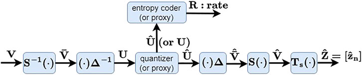
FIGURE 4. LVAC pipeline for compressing latents Z =[z_n]. Z is represented by difference latents V, normalized by S across levels and blocks to obtain $\bar{\mathbf{V}}$, divided by step sizes Δ across channels to obtain U, quantized by rounding to obtain $\widehat{\mathbf{U}}=\lfloor \mathbf{U}\rceil$, and reconstructed as $\widehat{\mathbf{Z}}={\mathbf{T}}_s\mathbf{S}\widehat{\mathbf{U}}\mathbf{\Delta }$. V (or equivalently $\bar{\mathbf{V}}$ in practice) is optimized by back-propagating through D (θ, Z)+ λR (θ, Z) and the pipeline using differentiable proxies for the quantizer and entropy coder.

As the quantizer and entropy encoder are not differentiable, they must be replaced by differentiable proxies during optimization. There are various differentiable proxies for the quantizer (Ballé et al., 2017; Agustsson and Theis, 2020; Luo et al., 2020), and we use the proxy

$Q\left(\mathbf{U}\right)=\mathbf{U}+\mathbf{W},(9)$

where W is iid unif (−0.5, 0.5). Various differentiable proxies for the entropy coder are also possible. As the number of bits in the entropy code for U = [u_m,c], we use the proxy $R(\mathbf{U})=-{\sum }_{m,c}{\log }_2{p}_{{\varphi }_{\ell ,c}}(u_{m,c})$, where

$p_{{\varphi }_{\ell ,c}}\left(u\right)={\text{CDF}}_{{\varphi }_{\ell ,c}}\left(u+0.5\right)-{\text{CDF}}_{{\varphi }_{\ell ,c}}\left(u-0.5\right)(10)$

(Ballé et al., 2017). The CDF is modeled by a neural network with parameters ϕ_ℓ,c that depend on the channel c and also the level ℓ (but not the offset n) of the coefficient u_m,c. At inference time, the bit rate is R(⌊U⌉) instead of R(U). These functions are provided by the Continuous Batched Entropy (cbe) model in (Ballé et al., 2021).

Note that the parameters Δ_c as well as the parameters ϕ_ℓ,c, for all ℓ and c, must be transmitted to the decoder. However, the overhead for transmitting Δ_c is negligible, and the overhead for transmitting ϕ_ℓ,c can be circumvented by using a backward-adaptive entropy code in its place at inference time. (See Section 5.4).

4.3 Coordinate based network

Any CBN can be used in the LVAC framework, but in our experiments we usually use a two-layer MLP,

$\mathbf{y}=f_{\theta }\left(\mathbf{x};\mathbf{z}\right)=\sigma \left({\mathbf{b}}^3+{\mathbf{W}}^{3\times H}\sigma \left({\mathbf{b}}^H+{\mathbf{W}}^{H\times \left(3+C\right)}\left[\mathbf{x},\mathbf{z}\right]\right)\right),(11)$

where θ = (b³, W^3×H, b^H, W^H×(3+C)), H is the number of hidden units, and σ(⋅) is pointwise rectification (ReLU). (Here we take x, y, and z to be column vectors instead of the row vectors we use elsewhere.) Note that there is no positional encoding of x. Alternatively, we use a two-layer position-attention (PA) network,

$\mathbf{y}=f_{\theta }\left(\mathbf{x};\mathbf{z}\right)={\mathbf{b}}^3+\mathbf{z}\odot \sin \left({\mathbf{b}}^C+{\mathbf{W}}^{C\times 3}\mathbf{x}\right),(12)$

where θ = (b³, b^C, W^C×3) and ⊙ is pointwise multiplication. The PA network is a simplified version of the modulated periodic activations in (Mehta et al., 2021), with many fewer parameters than MLPs while an efficient representation at low bit rates.

Once the latent vectors Z = [z_n] are decoded from $\widehat{\mathbf{U}}$ as $\widehat{\mathbf{Z}}=[{\widehat{\mathbf{z}}}_{\mathbf{n}}]$ and θ is decoded as $\widehat{\theta }$, the attributes $\widehat{\mathbf{y}}$ of any point $\mathbf{x}\in {\mathbb{R}}^3$ can be queried as illustrated in Figure 3.

5 Experimental results

5.1 Dataset and experimental details

Our dataset comprises (i) seven full human body voxelized point clouds derived from meshes created in (Guo et al., 2019; Meka et al., 2020) (shown in Figure 1) and (ii) seven point clouds—four full human bodies and three objects of art—from the MPEG PCC dataset (d’Eon et al., 2017; Alliez et al., 2017) (see the Supplementary Material). Integer voxel coordinates are used as the point positions x_i. The voxels (and hence the point positions) have 10-bit resolution. This results in an octree of depth 10, or alternatively a binary tree of depth 30, for every point cloud. For most experiments, we train all variables (latents, step sizes, an entropy model per binary level, and a CBN at the target level L) on a single point cloud, as the variables are specific to each point cloud. However, for the generalization experiments in Section 5.4, we train only the latents, step sizes, and entropy models on the given point cloud, while using a CBN pre-trained on a different point cloud. Additional experimental details are given in the Supplementary Material.

The entire point cloud constitutes one batch. All configurations are trained in about 25 K steps using the Adam optimizer and a learning rate of 0.01, with low bit rate configurations typically taking longer to converge. Each step takes 0.5–3.0 s on an NVIDIA P100 class GPU in eager mode with various debugging checks in place. We will open-source our code on https://github.com/tensorflow/compression/tree/master/models/lvac/upon publication.

As the experimental results below will show, the relative performance gains of various LVAC configurations and the baselines are largely consistent over all human body point clouds as well as object point clouds. This consistency may be explained in part by all variables in LVAC being trained on the given point cloud; hence LVAC is instance-adaptive (except in our generalization studies). No average-case models are trained to fit all point clouds. Thus we expect consistent behavior across other types of point clouds, e.g., room scans. We acknowledge, however, that some types of point clouds, such as dynamically-acquired LIDAR point clouds, may have a special structure that our framework does not take advantage of. Indeed, MPEG G-PCC has special coding modes for such point clouds.

5.2 Baselines

5.2.1 RAHT

Our first baseline is RAHT, which is the core transform in the MPEG G-PCC, coupled with the adaptive Run-Length Golomb-Rice (RLGR) entropy coder (Malvar, 2006). Figure 5A shows the rate-distortion (RD) performance of RAHT + RLGR in RGB PSNR (dB) vs. bit rate (bits per point, or bpp). As PSNR is a measure of quality, higher is better. In RAHT + RLGR, the RAHT coefficients are uniformly scalar quantized. The quantized coefficients are concatenated by level from the root to the leaves and entropy coded using RLGR, independently for each color component. The RD performances using RGB and YUV (BT.709) colorspaces are shown in Figure 5A in blue with filled and unfilled markers, respectively. At low bit rates, YUV provides a significant gain in RGB PSNR, but this falls off at high bit rates.

FIGURE 5

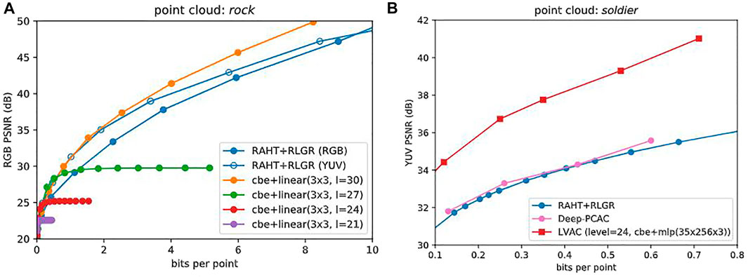
FIGURE 5. (A) Baselines. RAHT + RLGR (RGB) and (YUV) are shown against 3×3 linear models at levels 30, 27, 24, and 21, which optimize the colorspace by minimizing D + λR using the cbe entropy model. Since level = 30, model = cbe + linear(3x3) outperforms RAHT + RLGR (YUV) we discard the latter and use the others as baselines for more complex CBNs. (B) RD performance (YUV PSNR vs bit rate) comparison with RAHT + RLGR (RGB) (de Queiroz and Chou, 2016) and Deep-PCAC (Sheng et al., 2021).

5.2.2 Deep-PCAC

As a secondary baseline, we provide a comparison with Deep-PCAC (Sheng et al., 2021)—see Figure 5B. As mentioned earlier, Deep-PCAC is based on PointNet, which is not volumetric. Therefore, it cannot be used for other scenarios such as radiance fields and also lacks point cloud features such as infinite zoom. We still compare LVAC with Deep-PCAC just to show that learned point cloud attribute compression is not trivial and requires all the crucial steps that we discussed in this work.

5.2.3 Linear LVAC

Finally, level = 30, model = cbe + linear (3 × 3) in Figure 5A shows the RD performance of our LVAC framework when 3-channel latents (C = 3) are quantized and entropy coded using the Continuous Batched Entropy (cbe) model with the Noisy Deep Factorized prior from Tensorflow Compression (Ballé et al., 2021) followed by a simple 3 × 3 linear matrix as the CBN, at binary target level 30. The performance of this simple linear model agrees with that of RAHT-RLGR (YUV) at low rates, and outperforms it at high rates. Therefore, it is useful as a pseudo baseline and we show it in all subsequent plots along with our first baseline RAHT-RLGR (RGB). Figure 5A also shows that at lower target levels (27, 24, 21), LVAC with the 3 × 3 matrix saturates at high rates, since the 3 × 3 matrix has no positional input, and thus represents the volumetric attribute function as a constant across each block. These constant functions serve as baselines for more complex CBNs at these levels, described next.

Similar observations can be made from the plots in the Supplementary Material for the ten other point clouds. Alternative baselines are considered in Section 5.9.

5.3 Coordinate based networks

We now compare configurations of the LVAC framework with four different CBNs: linear(3x3) with 9 parameters (as a baseline), mlp(35 × 256 × 3) with 9,987 parameters, mlp(35 × 64 × 3) with 2,499 parameters, and pa(3 × 32 × 3) with 227 parameters, at different target levels. The mlp(35 × 256 × 3) and mlp(35 × 64 × 3) CBNs are two-layer MLPs with 35 inputs (3 for position and 32 for a latent vector, i.e., C = 32) and 3 outputs, having respectively 256 and 64 hidden nodes. The pa(3 × 32 × 3) CBN is a Position-Attention (PA) network also with 35 inputs (3 for position and 32 for a latent vector) and 3 outputs. All configurations use the Continuous Batched Entropy (cbe) model for quantization and entropy coding of the 32-channel latents.

Figures 6A–C shows (in green, red, purple) the RD performance of these CBNs at different target levels (27, 24, 21), along with the baselines (in blue, orange). We observe that first, at each target level L = 27, 24, 21, the CBNs with more parameters outperform the CBNs with fewer parameters. In particular, especially at higher bit rates, the MLP and PA networks at level L improve more than 5–10 dB over the linear network at level L, whose RD performance saturates as described earlier, for each L. Second, at each target level L = 27, 24, 21, there is a range of bit rates over which the MLP and PA networks improve by 2–3 dB over even the level = 30, model = cbe + linear(3x3) baseline, which does not saturate. The range of bit rates in which this improvement is achieved is higher for level 27, and lower for level 21, reflecting that higher quality requires CBNs with smaller blocksizes. In the Supplementary Material, we show these same data factored by CBN type instead of by level, to illustrate again that for each CBN type, each level is optimal for a different bit rate range. Figure 5B demonstrates that LVAC provides a gain of 2–5 dB over our secondary baseline, Deep-PCAC (Sheng et al., 2021). Comparison plots for other point clouds are provided in the Supplementary Material.

FIGURE 6

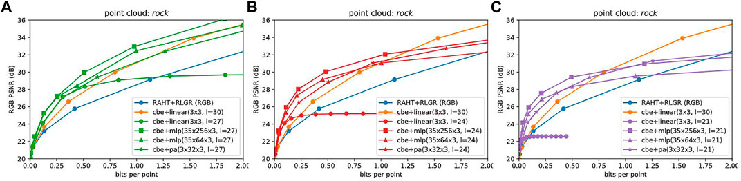
FIGURE 6. Coordinate Based Networks, by target level. (A–C) each show mlp(35 × 256 × 3), mlp(35 × 64 × 3), and pa(3 × 32 × 3) CBNs, along with baselines, at levels 27, 24, 21. More complex CBNs outperform less complex. Higher levels are better for higher bit rates.

The nature of a volumetric function f_θ(x; z) represented by a CBN is illustrated in Figure 7. To illustrate, we select the CBN mlp(35 × 256 × 3) trained on the rock point cloud at target level L = 21, and we plot cuts through the volumetric function f_θ(⋅; z) represented by this CBN. Specifically, let n be a randomly selected node at the target level L, let ${\widehat{\mathbf{z}}}_n$ be the quantized cumulative latent at that node, and let x_n = (x_n, y_n, z_n) be the position of a randomly selected point within the block at that node. Then we plot the first (red) component of the function $f_{\theta }(\mathbf{x};{\widehat{\mathbf{z}}}_n)$, where x varies from (0, y_n, z_n) to (N_x, y_n, z_n), where N_x is the width of a block at level L. We do this for many randomly selected nodes n to get a sense of the distribution of volumetric functions represented at that level. (The distribution looks similar for green and blue components, and for cuts along y and z axes.) We observe that for many values of ${\widehat{\mathbf{z}}}_n$, $f_{\theta }(\cdot ;{\widehat{\mathbf{z}}}_n)$ is a roughly constant function. Thus, ${\widehat{\mathbf{z}}}_n$ must encode the colors of the palette used for these functions. However, we also observe that for some values of ${\widehat{\mathbf{z}}}_n$, $f_{\theta }(\cdot ;{\widehat{\mathbf{z}}}_n)$ is a ramp or some other nonlinear function across its domain. Finally, we observe almost no energy at frequencies higher than the Nyquist frequency (half the sampling rate), where the sampling occurs at units of voxels. We conclude that $f_{\theta }(\cdot ;\widehat{\mathbf{z}})$ acts like a codebook of volumetric functions defined on N_x × N_y × N_z, fit to the point cloud at hand.

FIGURE 7

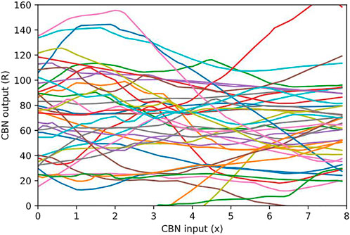
FIGURE 7. Cuts through the volumetric function (R, G, B)= f_θ((x, y_n, z_n); z_n) represented by a CBN, along the x-axis through a random point x_n =(x_n, y_n, z_n) in the point cloud within a node n, for various occupied nodes n at target level 21. It can be seen that the CBN specifies a codebook of volumetric functions defined on blocks, fit to the point cloud at hand.

5.4 Generalization

We also explore the degree to which the CBNs can be generalized across point clouds; that is, whether they can be trained to represent a universal family of volumetric functions. Figure 8 below show that the CBNs can indeed generalize across point clouds at low bit rates. We provide the corresponding plots for other point clouds in the Supplementary Material.

FIGURE 8

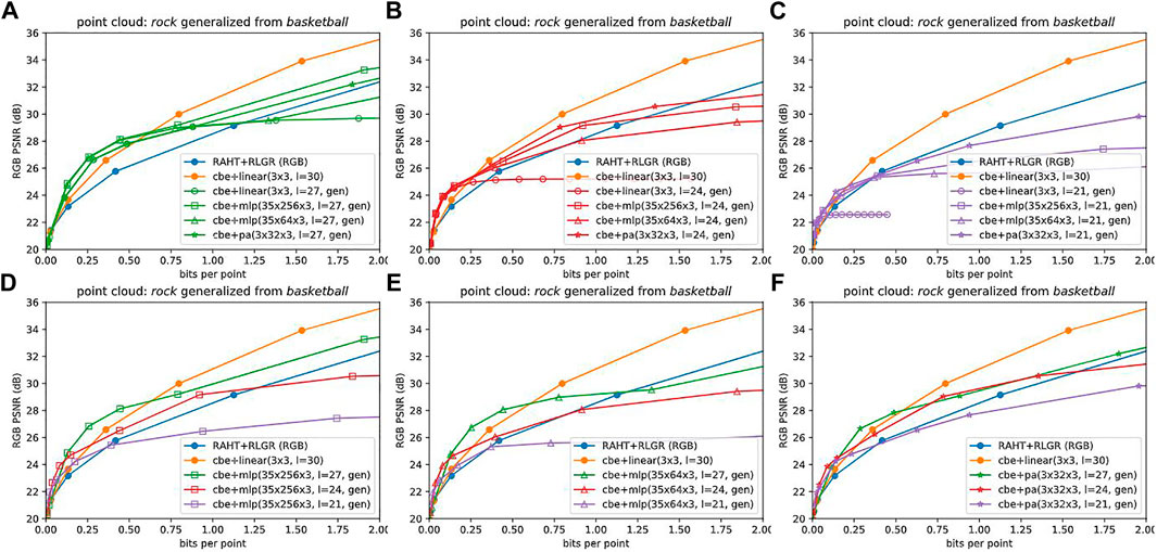
FIGURE 8. Coordinate Based Networks with generalization, by level (A–C) and by network (D–F). CBNs that are generalized (i.e., pre-trained on another point cloud) are able to outperform the baselines at low bit rates.

5.5 Side information

When the latents, step sizes, entropy models, and CBN are all optimized for a specific point cloud, quantizing and entropy coding only the latent vectors [z_n] is insufficient for reconstructing the point cloud attributes. The step sizes [Δ_c], entropy model parameters [ϕ_ℓ,c], and CBN parameters θ must also be quantized, entropy coded, and sent as side information. Sending side information incurs additional bit rate and distortion. Note that the side information for the step sizes is negligible, as there is only one step size for each of C = 32 channels.

5.5.1 Side information for the entropy models

We first consider the side information for the entropy models. Figure 9 shows the penalty required to transmit side information, for the entropy model for point cloud rock. We use the Tensorflow Compression’s Continuous Batched Entropy (cbe) model with the Noisy Deep Factorized prior. For 32 channels, this model has 23,296 parameters. If each parameter is represented with 32 bits, then 0.89 bits per point of side information is required for the point cloud rock, which has 837, 434 points. This would shift the RD performance from the solid green line to the dashed green line in the figure, for level = 27, model = cbe + mlp(35 × 256 × 3). However, fortunately, this costly side information can be avoided, by using cbe during training but using the adaptive Run-Length Golomb-Rice (RLGR) entropy coder Malvar (2006) during inference time. Since RLGR is backward adaptive, it can adapt to Laplacian-like distributions without sending any side information. Of course its coding efficiency may suffer, but our experiments show that this degradation is almost negligible. Henceforth we report RD performance using only RLGR. The resulting RD performance is shown in the dotted line with unfilled markers—an almost negligible degradation. The corresponding plots for other point clouds are given in the Supplementary Material.

FIGURE 9

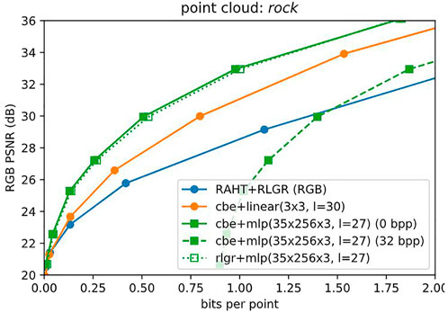
FIGURE 9. Side information for entropy model. Sending 32 bits per parameter for the cbe entropy model would reduce RD performance from solid to dashed green lines. But the backward-adaptive RLGR entropy coder (dotted, unfilled) obviates the need to send side information with almost no loss in performance.

5.5.2 Side information for the CBNs

Next, we consider the side information for the CBNs. For each point cloud, there is one CBN, at the target level L. Allocating 32 bits per floating point parameter would give the most pessimistic estimate for the side information. However, it is likely that 32 bits per floating point parameter is an order of magnitude more than necessary. Prior work has shown that simple model compression can be performed at 8 bits (Banner et al., 2018; Wang et al., 2018; Sun et al., 2019) or even more aggressively at 1–4 bits per floating point parameter (Han et al., 2015; Xu et al., 2018; Oktay et al., 2019; Stock et al., 2019; Wang et al., 2019; Isik et al., 2021a; Isik et al., 2022) with very low loss in performance, even with CBNs such as NeRF (Bird et al., 2021; Isik, 2021). Alternatively, the CBNs may be generalized by pre-training on other point clouds to avoid having to transmit any side information. Figure 10 shows RD performance under the 32-bit assumption as well as under generalization. We refer the reader to the Supplementary Material for the corresponding plots for other point clouds.

FIGURE 10

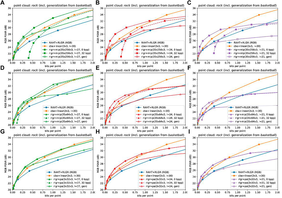
FIGURE 10. Effect of side information for coordinate based networks mlp(35 × 256 × 3) (A–C), mlp(35 × 64 × 3) (D–F), and pa(3 × 32 × 3) (G–I) at levels 27 (A,D,G), 24 (B,E,H), and 21 (C,F,I). Sending 32 bits per parameter for the CBN would degrade RD performance from solid to dashed lines. The degradation would be inversely proportional to compression ratio if model compression is used. Alternatively, generalization (pre-training the CBN on one or more other point clouds), which works well at low bit rates, would obviate the need to transmit any side information. Generalization is indicated by “gen” in the legend.

Now, we turn to a key ablation study.

5.6 Orthonormalization

One of our main contributions is to show that naïve uniform scalar quantization and entropy coding of the latents leads to poor results, and that properly normalizing the coefficients before quantization achieves over a 30% reduction in bit rate. In this ablation study, we remove our orthonormalization by setting the scale matrix S in (Eqs. 7, 8) and Figure 4 to the identity matrix, thus removing any dependency of the attribute compression on the geometry. This corresponds to a naïve approach to compression, for example by assuming a fixed number of bits per latent as in (Takikawa et al., 2021). Table 1 shows that compared to this naïve approach, our normalization achieves over 30% reduction in bit rate (computed using (Bjøntegaard, 2001; Pateux and Jung, 2007)). This quantifies the reduction in bit rate due to conditioning the attribute compression on the geometry. We give the results averaged over all point clouds in Table 1, results for rock point cloud in Figure 11, and provide results for each point cloud in the Supplementary Material.

TABLE 1

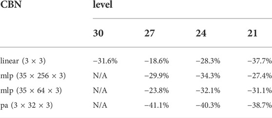
TABLE 1. BD-Rate reductions due to normalization, averaged over point clouds. Normalization is crucial for good performance. Without normalization, there is no dependence on geometry.

FIGURE 11

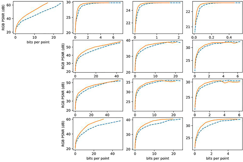
FIGURE 11. RD performance improvement due to normalization, corresponding to entries in Table 1, i.e., columns 1, 2, 3, 4 correspond to levels 30, 27, 24, 21, respectively, and rows 1, 2, 3, 4 correspond to linear(3x3), mlp(35 × 256 × 3), mlp(35 × 64 × 3), pa(3 × 32 × 3), respectively.

5.7 Convex hull

For different bit rate ranges and for different assumptions on the cost of side information, different configurations of the LVAC framework may be optimal. Figure 12 shows the convex hull, or Pareto fontier, of all configurations under various assumptions of 0 (Figure 12A), 8 (Figure 12B), and 32 (Figure 12C) bits per floating point parameter. All configurations that we have examined in this paper appear in Figure 12. However, only those that participate in the convex hull appear in the legend and are plotted with a solid line. (The others are dotted.) The convex hull is 2–4 dB over the baselines. We observe: first, when the side information costs nothing (0 bits per parameter), the convex hull contains exclusively the largest CBN (mlp(35 × 256 × 3)), at higher target levels for higher bit rates. Second, as the cost of the side information increases, the smaller CBNs (mlp(35 × 64 × 3) and pa(3 × 32 × 3)) begin to participate in the convex hull, especially at lower bit rates. Eventually, at 32 bits per parameters, the largest CBN is excluded entirely. Third, the generalizations never participate in the convex hull, despite not incurring any penalty due to side information. This could be because they are trained only on a single other point cloud in these experiments. Training the CBNs on more representative data would probably improve their generalization performance but is left for future work. The corresponding plots for other points clouds are provided in the Supplementary Material.

FIGURE 12

FIGURE 12. Convex hull (solid black line) of RD performances of all CBN configurations across all levels, including side information using 0 (A), 8 (B), and 32 (C) bits per CBN parameter. Configurations that participate in the convex hull are listed, with baselines, in the legend and appear as solid lines. Others are dotted. At 0 bits per parameter (bpp), the more complex CBNs dominate. At higher bpp, the less complex CBNs begin to participate, especially at lower bit rates. CBNs generalized from another point cloud never participate.

5.8 Subjective quality

Figure 13 shows compression quality at around 0.25 bpp, under the assumption of 0 bits per floating point parameter. Additional bit rates are shown in the Supplementary Material.

FIGURE 13

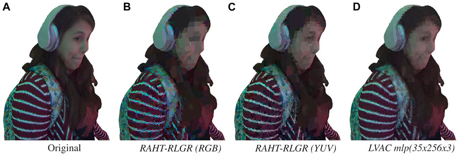
FIGURE 13. Subjective quality around 0.25 bpp. (A) Original. (B) 0.258 bpp, 24.6 dB. (C) 0.255 bpp, 25.9 dB. (D) 0.255 bpp, 28.0 dB.

5.9 Baselines, revisited

We now return to the matter of baselines. Figure 14 shows our previous baseline, RAHT + RLGR, for both RGB and YUV colorspaces (blue lines). Although RAHT is the transform used in MPEG G-PCC, the reference software TMC13 v6.0 (July 2019) offers improved RD performance (green lines) compared to RAHT + RLGR, due principally to better entropy coding. In particular, TMC13 uses context-adaptive binary arithmetic coding with various coding modes, while RAHT + RLGR uses RLGR. We use RAHT + RLGR as our baseline because our experiments use RLGR as our entropy coder; the specific entropy coder used in TMC13 is difficult to extract from the standard. The latest version, TMC13 v14.0 (October 2021), offers even better RD performance, by introducing for example joint coding modes for color channels that are all zero (orange lines). It also introduces predictive RAHT, in which the RAHT coefficients at each level are predicted from the decoded RAHT coefficients at the previous level (Lasserre and Flynn, 2019; 3DG, 2020b; Pavez et al., 2021). The prediction residuals, instead of the RAHT coefficients themselves, are quantized and entropy coded. Predictive RAHT alone improves RD performance by 2–3 dB (red lines). Nevertheless, in the low bit rate regime, LVAC with RLGR and no RAHT prediction has better performance than even TMC13 v14.0 with predictive RAHT (solid black line, from Figure 12A). We believe that the RD performance of LVAC can be further improved significantly. In particular, the principal advances of TMC13 over RAHT + RLGR—better entropy coding and predictive RAHT—are equally applicable to the LVAC framework. For example, better entropy coding could be done with a hyperprior (Ballé et al., 2018), and predictive RAHT could be applied to the latent vectors. These explorations are left for future work.

FIGURE 14

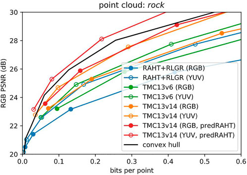
FIGURE 14. Baselines, revisited. In both RGB and YUV color spaces, MPEG G-PCC reference software TMC13 v6.0 improves over RAHT + RLGR, primarily due to context-adaptive (i.e., dependent) entropy coding. TMC13 v14.0 improves still further, primarily due to predictive RAHT. LVAC (black line, from Figure 12A) outperforms all but TMC13 v14.0. However, better entropy coding (e.g., hyperprior) and predictive RAHT can also be applied to LVAC.

6 Discussion and conclusion

This work is the first to compress volumetric functions y = f_θ(x) modeled by local coordinate-based networks. Though we focused on RGB attributes y, the extension to other attributes (signed distance, density, etc.) is straightforward. Also, though we focused on $\mathbf{x}\in {\mathbb{R}}^3$, extensions to hyper-volumetric functions (such as y = f_θ(x, d) where d is a view direction) is also straightforward. Thus LVAC should be applicable to plenoptic point clouds (Krivokuca et al., 2018; Sandri et al., 2018; Zhang et al., 2018; Sandri et al., 2019; Zhang et al., 2019) as well as radiance fields (Mildenhall et al., 2020; Yu A. et al., 2021; Martel et al., 2021; Takikawa et al., 2021; Zhang et al., 2021) under an appropriate distance measure. We believe that the main difference between plenoptic point clouds and radiance fields is the distortion measure d (f, f_θ). For point clouds, d (f, f_θ) is measured in the domain of f, such as the MSE between colors on points in 3D. For radiance fields, d (f, f_θ) is measured in the domain of projections or renderings of f onto 2D images, such as the MSE between colors of pixels that are renderings of f and f_θ onto 2D images. In (de Queiroz and Chou, 2017), the former distortion measures are called matching distortions, while the latter are called projection distortions. A change in distortion measure may be all that is required to apply LVAC properly to radiance field compression. This work is also among the first to compress point cloud attributes using neural networks, outperforming RAHT, used in MPEG G-PCC, by 2–4 dB and Deep-PCAC, a recent learned compression framework, by 2–5 dB. Although MPEG G-PCC uses additional coding tools to further improve compression, such as context adaptive arithmetic coding, joint entropy coding of color, and predictive RAHT, these tools are also at our disposal, and may be the subject of further work. It should be recalled that learned image compression evolved over dozens of papers and a half dozen years, being competitive at first with only JPEG on thumbnails, and then successively with JPEG-2000, WebP, and BGP. Only recently has learned image compression been able to outperform the latest standard, VVC, in PSNR (Guo et al., 2021). Learned volumetric attribute compression (LVAC), like learned image compression, is a work in progress.

Data availability statement

Publicly available datasets were analyzed in this study. This data can be found here: JPEG Pleno Database: 8i Voxelized Full Bodies (8iVFB v2)—A Dynamic Voxelized Point Cloud Dataset: http://plenodb.jpeg.org/pc/8ilabs/.

Ethics statement

Written informed consent was obtained from the individual(s) for the publication of any potentially identifiable images or data included in this article.

Author contributions

PC proposed the initial idea, BI finalized the proposed framework and implemented it. BI and PC wrote the paper. SH, NJ, and GT helped with the implementation and writing.

Acknowledgments

The authors would like to thank Eirikur Agustsson and Johannes Ballé for helpful discussions.

Conflict of interest

Authors PC, SH, NJ, and GT were employed by the company Google.

The remaining author declares that the research was conducted in the absence of any commercial or financial relationships that could be construed as a potential conflict of interest.

Publisher’s note

All claims expressed in this article are solely those of the authors and do not necessarily represent those of their affiliated organizations, or those of the publisher, the editors and the reviewers. Any product that may be evaluated in this article, or claim that may be made by its manufacturer, is not guaranteed or endorsed by the publisher.

Supplementary material

The Supplementary Material for this article can be found online at: https://www.frontiersin.org/articles/10.3389/frsip.2022.1008812/full#supplementary-material

Footnotes

¹We train the latents, quantizer stepsizes, neural entropy model, and the CBNs for each point cloud. However, we show the CBNs could be generalized across different point clouds.

References

Agustsson, E., and Theis, L. (2020). “Universally quantized neural compression,” in Advances in Neural Information Processing Systems.

Google Scholar

Alliez, P., Forge, F., De Luca, L., Pierrot-Deseilligny, M., and Preda, M. (2017). Culture 3D cloud: A cloud computing platform for 3D scanning, documentation, preservation and dissemination of cultural heritage. Hal 64.

Google Scholar

Balle, J., Chou, P. A., Minnen, D., Singh, S., Johnston, N., Agustsson, E., et al. (2020). Nonlinear transform coding. IEEE J. Sel. Top. Signal Process. 1, 339–353. doi:10.1109/JSTSP.2020.3034501

CrossRef Full Text | Google Scholar

Ballé, J. (2018). Efficient nonlinear transforms for lossy image compression. 2018 Picture Coding Symp. San Francisco, CA, United States: PCS. doi:10.1109/PCS.2018.8456272

CrossRef Full Text | Google Scholar

Ballé, J., Hwang, S. J., and Agustsson, E. (2021). TensorFlow compression: Learned data compression. Availableat: http://github.com/tensorflow/compression.

Google Scholar

Ballé, J., Laparra, V., and Simoncelli, E. P. (2016). End-to-end optimization of nonlinear transform codes for perceptual quality. Picture Coding Symp. Nuremberg, Germany: PCS. doi:10.1109/PCS.2016.7906310

CrossRef Full Text | Google Scholar

Ballé, J., Laparra, V., and Simoncelli, E. P. (2017). “End-to-end optimized image compression,” in 5th Int. Conf. on Learning Representations (ICLR).

Google Scholar

Ballé, J., Minnen, D., Singh, S., Hwang, S. J., and Johnston, N. (2018). “Variational image compression with a scale hyperprior,” in 6th Int. Conf. on Learning Representations (ICLR).

Google Scholar

Banner, R., Hubara, I., Hoffer, E., and Soudry, D. (2018). “Scalable methods for 8-bit training of neural networks,” in Proceedings of the 32nd International Conference on Neural Information Processing Systems, 5151–5159.

Google Scholar

Barron, J. T., Mildenhall, B., Tancik, M., Hedman, P., Martin-Brualla, R., and Srinivasan, P. P. (2021). Mip-nerf: A multiscale representation for anti-aliasing neural radiance fields. ArXiv. doi:10.48550/arXiv.2103.13415

CrossRef Full Text | Google Scholar

Bird, T., Ballé, J., Singh, S., and Chou, P. A. (2021). “3d scene compression through entropy penalized neural representation functions,” in Picture Coding Symposium (PCS).

CrossRef Full Text | Google Scholar

Bjøntegaard, G. (2001). Calculation of average PSNR differences between RD-curves. Austin, Texas. Technical Report VCEG-M33, ITU-T SG16/Q6.

Google Scholar

Chen, Y., Liu, S., and Wang, X. (2021). “Learning continuous image representation with local implicit image function,” in Proceedings of the IEEE/CVF conference on computer vision and pattern recognition, 8628–8638.

CrossRef Full Text | Google Scholar

Cheng, Z., Sun, H., Takeuchi, M., and Katto, J. (2020). “Learned image compression with discretized Gaussian mixture likelihoods and attention modules,” in Proceedings of the IEEE/CVF Conference on Computer Vision and Pattern Recognition, 7939–7948.

CrossRef Full Text | Google Scholar

Chou, P. A., Koroteev, M., and Krivokuća, M. (2020). A volumetric approach to point cloud compression—Part i: Attribute compression. IEEE Trans. Image Process. 29, 2203–2216. doi:10.1109/TIP.2019.2908095

CrossRef Full Text | Google Scholar

Cohen, R. A., Tian, D., and Vetro, A. (2016). “Attribute compression for sparse point clouds using graph transforms,” in IEEE Int’l Conf. Image Processing (ICIP).

CrossRef Full Text | Google Scholar

de Queiroz, R. L., and Chou, P. A. (2016). Compression of 3d point clouds using a region-adaptive hierarchical transform. IEEE Trans. Image Process. 25, 3947–3956. doi:10.1109/TIP.2016.2575005

PubMed Abstract | CrossRef Full Text | Google Scholar

de Queiroz, R. L., and Chou, P. A. (2017). Motion-compensated compression of dynamic voxelized point clouds. IEEE Trans. Image Process. 26, 3886–3895. doi:10.1109/TIP.2017.2707807

PubMed Abstract | CrossRef Full Text | Google Scholar

d’Eon, E., Harrison, B., Meyers, T., and Chou, P. A. (2017). 8i voxelized full bodies — a voxelized point cloud dataset. Input document M74006 & m42914. Ljubljana, Slovenia: JPEG & MPEG. ISO/IEC JTC1/SC29 WG1 & WG11.

Google Scholar

DeVries, T., Bautista, M. A., Srivastava, N., Taylor, G. W., and Susskind, J. M. (2021). Unconstrained scene generation with locally conditioned radiance fields.

Google Scholar

DG 3 (2020a). Final call for evidence on JPEG Pleno point cloud coding. Approved WG 1 document N88014. ISO/IEC MPEG JTC1/SC29/WG1, online.

Google Scholar

DG 3 (2020b). G-PCC Codec Description v12. Approved WG 11 document N18891. Geneva, CH. ISO/IEC MPEG JTC1/SC29/WG11.

Google Scholar

Fang, G., Hu, Q., Wang, H., Xu, Y., and Guo, Y. (2020). “3dac: Learning attribute compression for point clouds,” in 2022 IEEE/CVF Conf. on Computer Vision and Pattern Recognition (CVPR).

Google Scholar

Fujiwara, K., and Hashimoto, T. (2020). “Neural implicit embedding for point cloud analysis,” in Proceedings of the IEEE/CVF Conference on Computer Vision and Pattern Recognition, 11734–11743.

CrossRef Full Text | Google Scholar

Graziosi, D., Nakagami, O., Kuma, S., Zaghetto, A., Suzuki, T., and Tabatabai, A. (2020). An overview of ongoing point cloud compression standardization activities: Video-based (v-pcc) and geometry-based (g-pcc). APSIPA Trans. Signal Inf. Process. 9, e13. doi:10.1017/ATSIP.2020.12

CrossRef Full Text | Google Scholar

Guarda, A. F. R., Rodrigues, N. M. M., and Pereira, F. (2019a). “Deep learning-based point cloud coding: A behavior and performance study,” in 2019 8th European Workshop on Visual Information Processing (EUVIP), 34–39. doi:10.1109/EUVIP47703.2019.8946211

CrossRef Full Text | Google Scholar

Guarda, A. F. R., Rodrigues, N. M. M., and Pereira, F. (2020). “Deep learning-based point cloud geometry coding: RD control through implicit and explicit quantization,” in 2020 IEEE Int. Conf. on Multimedia & Expo Wksps. (ICMEW). doi:10.1109/ICMEW46912.2020.9106022

CrossRef Full Text | Google Scholar

Guarda, A. F. R., Rodrigues, N. M. M., and Pereira, F. (2019b). “Point cloud coding: Adopting a deep learning-based approach,” in 2019 Picture Coding Symposium (PCS), 1–5. doi:10.1109/PCS48520.2019.8954537

CrossRef Full Text | Google Scholar

Guo, K., Lincoln, P., Davidson, P., Busch, J., Yu, X., Whalen, M., et al. (2019). The relightables: Volumetric performance capture of humans with realistic relighting. ACM Trans. Graph. 38, 1–19. doi:10.1145/3355089.3356571

CrossRef Full Text | Google Scholar

Guo, Z., Zhang, Z., Feng, R., and Chen, Z. (2021). Causal contextual prediction for learned image compression. IEEE Trans. Circuits Syst. Video Technol. 1, 2329–2341. doi:10.1109/TCSVT.2021.3089491

CrossRef Full Text | Google Scholar

Han, S., Mao, H., and Dally, W. J. (2015). Deep compression: Compressing deep neural networks with pruning, trained quantization and huffman coding. arXiv preprint arXiv:1510.00149.

Google Scholar

Hedman, P., Srinivasan, P. P., Mildenhall, B., Barron, J. T., and Debevec, P. (2021). “Baking neural radiance fields for real-time view synthesis,” in Proceedings of the IEEE/CVF International Conference on Computer Vision, 5875–5884.

CrossRef Full Text | Google Scholar

Hu, Y., Yang, W., Ma, Z., and Liu, J. (2021). “Learning end-to-end lossy image compression: A benchmark,” in IEEE Transactions on Pattern Analysis and Machine Intelligence.

CrossRef Full Text | Google Scholar

Isik, B., Choi, K., Zheng, X., Weissman, T., Ermon, S., Wong, H.-S. P., et al. (2021a). Neural network compression for noisy storage devices. NeurIPS deep learning through information geometry workshop. arXiv:2102.07725.

Google Scholar

Isik, B., Chou, P. A., Hwang, S. J., Johnston, N., and Toderici, G. (2021b). Lvac: Learned volumetric attribute compression for point clouds using coordinate based networks. arXiv preprint arXiv:2111.08988.

Google Scholar

Isik, B. (2021). “Neural 3d scene compression via model compression,” in IEEE Conf. on Computer Vision and Pattern Recognition (CVPR) WiCV Workshop. arXiv:2105.03120.

Google Scholar

Isik, B., Weissman, T., and No, A. (2022). “An information-theoretic justification for model pruning,” in Proceedings of The 25th International Conference on Artificial Intelligence and Statistics of Proceedings of Machine Learning Research (Valencia, Spain: PMLR), 3821–3846.

Google Scholar

Jang, E. S., Preda, M., Mammou, K., Tourapis, A. M., Kim, J., Graziosi, D. B., et al. (2019). Video-based point-cloud-compression standard in mpeg: From evidence collection to committee draft [standards in a nutshell]. IEEE Signal Process. Mag. 36, 118–123. doi:10.1109/MSP.2019.2900721

CrossRef Full Text | Google Scholar

Knodt, J., Baek, S.-H., and Heide, F. (2021). Neural ray-tracing: Learning surfaces and reflectance for relighting and view synthesis. arXiv preprint arXiv:2104.13562.

Google Scholar

Krivokuća, M., Chou, P. A., and Koroteev, M. (2020). A volumetric approach to point cloud compression–part ii: Geometry compression. IEEE Trans. Image Process. 29, 2217–2229. doi:10.1109/TIP.2019.2957853

CrossRef Full Text | Google Scholar

Krivokuca, M., Chou, P. A., and Savill, P. (2018). 8i voxelized surface light field (8iVSLF) dataset. Input document m42914. Ljubljana, Slovenia. ISO/IEC JTC1/SC29 WG11 (MPEG).

Google Scholar

Krivokuca, M., Miandji, E., Guillemot, C., and Chou, P. (2021). Compression of plenoptic point cloud attributes using 6-d point clouds and 6-d transforms. IEEE Trans. Multimed., 1. doi:10.1109/tmm.2021.3129341

CrossRef Full Text | Google Scholar

Kundu, A., Genova, K., Yin, X., Fathi, A., Pantofaru, C., Guibas, L., et al. (2022a). “Panoptic neural fields: A semantic object-aware neural scene representation,” in Cvpr.

CrossRef Full Text | Google Scholar

Kundu, A., Genova, K., Yin, X., Fathi, A., Pantofaru, C., Guibas, L. J., et al. (2022b). “Panoptic neural fields: A semantic object-aware neural scene representation,” in Proceedings of the IEEE/CVF Conference on Computer Vision and Pattern Recognition (New Orleans, Louisiana, United States: CVPR), 12871–12881.

CrossRef Full Text | Google Scholar

Lasserre, S., and Flynn, D. (2019). On an improvement of RAHT to exploit attribute correlation. input document m47378. Geneva, CH. ISO/IEC MPEG JTC1/SC29/WG11.

Google Scholar

Lazzarotto, D., Alexiou, E., and Ebrahimi, T. (2021). “On block prediction for learning-based point cloud compression,” in 2021 IEEE International Conference on Image Processing (Anchorage, Alaska, United States: ICIP), 3378–3382. doi:10.1109/ICIP42928.2021.9506429

CrossRef Full Text | Google Scholar

Luo, X., Talebi, H., Yang, F., Elad, M., and Milanfar, P. (2020). The rate-distortion-accuracy tradeoff: Jpeg case study. arXiv preprint arXiv:2008.00605.

Google Scholar

Malvar, H. (2006). “Adaptive run-length/golomb-rice encoding of quantized generalized Gaussian sources with unknown statistics,” in Data Compression Conference (DCC’06), 23–32.

Google Scholar

Martel, J. N., Lindell, D. B., Lin, C. Z., Chan, E. R., Monteiro, M., and Wetzstein, G. (2021). Acorn: Adaptive coordinate networks for neural scene representation. arXiv preprint arXiv:2105.02788

Google Scholar

Mehta, I., Gharbi, M., Barnes, C., Shechtman, E., Ramamoorthi, R., and Chandraker, M. (2021). “Modulated periodic activations for generalizable local functional representations,” in Proceedings of the IEEE/CVF International Conference on Computer Vision, 14214–14223.

CrossRef Full Text | Google Scholar

Meka, A., Pandey, R., Haene, C., Orts-Escolano, S., Barnum, P., Davidson, P., et al. (2020). Deep relightable textures - volumetric performance capture with neural rendering. ACM Trans. Graph. 39, 1–21. doi:10.1145/3414685.3417814

CrossRef Full Text | Google Scholar

Mekuria, R., Blom, K., and Cesar, P. (2017). Design, implementation, and evaluation of a point cloud codec for tele-immersive video. IEEE Trans. Circuits Syst. Video Technol. 27, 828–842. doi:10.1109/tcsvt.2016.2543039

CrossRef Full Text | Google Scholar

Mentzer, F., Toderici, G. D., Tschannen, M., and Agustsson, E. (2020). High-fidelity generative image compression. Adv. Neural Inf. Process. Syst. 33.

Google Scholar

Mescheder, L., Oechsle, M., Niemeyer, M., Nowozin, S., and Geiger, A. (2019). “Occupancy networks: Learning 3d reconstruction in function space,” in Proceedings IEEE Conf. on Computer Vision and Pattern Recognition (CVPR).

CrossRef Full Text | Google Scholar

Milani, S. (2020). “A syndrome-based autoencoder for point cloud geometry compression,” in 2020 IEEE International Conference on Image Processing (Abu Dhabi, United Arab Emirates: ICIP), 2686–2690. doi:10.1109/ICIP40778.2020.9190647

CrossRef Full Text | Google Scholar

Milani, S. (2021). “Adae: Adversarial distributed source autoencoder for point cloud compression,” in 2021 IEEE International Conference on Image Processing (Anchorage, Alaska, United States: ICIP), 3078–3082. doi:10.1109/ICIP42928.2021.9506750

CrossRef Full Text | Google Scholar

Mildenhall, B., Srinivasan, P. P., Tancik, M., Barron, J. T., Ramamoorthi, R., and Ng, R. (2020). “Nerf: Representing scenes as neural radiance fields for view synthesis,” in Eccv.

CrossRef Full Text | Google Scholar

Minnen, D., Ballé, J., and Toderici, G. (2018). Joint autoregressive and hierarchical priors for learned image compression. Adv. Neural Inf. Process. Syst. 31.

Google Scholar

Oktay, D., Ballé, J., Singh, S., and Shrivastava, A. (2019). “Scalable model compression by entropy penalized reparameterization,” in International Conference on Learning Representations.

Google Scholar

Park, J., Chou, P. A., and Hwang, J. (2019a). Rate-utility optimized streaming of volumetric media for augmented reality. IEEE J. Emerg. Sel. Top. Circuits Syst. 9, 149–162. doi:10.1109/JETCAS.2019.2898622

CrossRef Full Text | Google Scholar

Park, J., Florence, P., Straub, J., Newcombe, R., and Lovegrove, S. (2019b). “Deepsdf: Learning continuous signed distance functions for shape representation,” in 2019 IEEE/CVF Conference on Computer Vision and Pattern Recognition (CVPR), Long Beach, CA, USA, 15-20 June 2019 (IEEE), 165–174. doi:10.1109/CVPR.2019.00025

CrossRef Full Text | Google Scholar

Pateux, S., and Jung, J. (2007). An excel add-in for computing bjontegaard metric and its evolution. ITU-T SG16 Q. 6, 7.

Google Scholar

Pavez, E., Chou, P. A., de Queiroz, R. L., and Ortega, A. (2018). Dynamic polygon clouds: Representation and compression for VR/AR. APSIPA Trans. Signal Inf. Process. 7, e15. doi:10.1017/ATSIP.2018.15

CrossRef Full Text | Google Scholar

Pavez, E., Souto, A. L., Queiroz, R. L. D., and Ortega, A. (2021). “Multi-resolution intra-predictive coding of 3d point cloud attributes,” in 2021 IEEE International Conference on Image Processing (ICIP), 3393–3397. doi:10.1109/ICIP42928.2021.9506641

CrossRef Full Text | Google Scholar

Pierdicca, R., Paolanti, M., Matrone, F., Martini, M., Morbidoni, C., Malinverni, E. S., et al. (2020). Point cloud semantic segmentation using a deep learning framework for cultural heritage. Remote Sens. 12, 1005. doi:10.3390/rs12061005

CrossRef Full Text | Google Scholar

Quach, M., Valenzise, G., and Dufaux, F. (2020a). “Folding-based compression of point cloud attributes,” in 2020 IEEE International Conference on Image Processing (ICIP), 3309–3313. doi:10.1109/ICIP40778.2020.9191180

CrossRef Full Text | Google Scholar

Quach, M., Valenzise, G., and Dufaux, F. (2020b2020). “Improved deep point cloud geometry compression,” in IEEE 22nd International Workshop on Multimedia Signal Processing (MMSP), 1–6.

CrossRef Full Text | Google Scholar

Quach, M., Valenzise, G., and Dufaux, F. (2019). “Learning convolutional transforms for lossy point cloud geometry compression,” in 2019 IEEE Int. Conf. on Image Processing (ICIP). doi:10.1109/ICIP.2019.8803413

CrossRef Full Text | Google Scholar

Reiser, C., Peng, S., Liao, Y., and Geiger, A. (2021). “Kilonerf: Speeding up neural radiance fields with thousands of tiny mlps,” in Proceedings of the IEEE/CVF International Conference on Computer Vision, 14335–14345.

CrossRef Full Text | Google Scholar

Rematas, K., Liu, A., Srinivasan, P. P., Barron, J. T., Tagliasacchi, A., Funkhouser, T., et al. (2022). Urban radiance fields. New Orleans, Louisiana, United States: CVPR.

Google Scholar

Sandri, G., de Queiroz, R., and Chou, P. A. (2018). “Compression of plenoptic point clouds using the region-adaptive hierarchical transform,” in 25th IEEE Int. Conf. on Image Processing (Athens, Greece: ICIP), 1153–1157.

CrossRef Full Text | Google Scholar

Sandri, G., de Queiroz, R. L., and Chou, P. A. (2019). Compression of plenoptic point clouds. IEEE Trans. Image Process. 28, 1419–1427. doi:10.1109/tip.2018.2877486

CrossRef Full Text | Google Scholar

Sandri, G., Figueiredo, V. F., Chou, P. A., and de Queiroz, R. (2019a). “Point cloud compression incorporating region of interest coding,” in 2019 IEEE International Conference on Image Processing (ICIP), 4370–4374. doi:10.1109/ICIP.2019.8803553

CrossRef Full Text | Google Scholar

Sandri, G. P., Chou, P. A., Krivokuća, M., and de Queiroz, R. L. (2019b). Integer alternative for the region-adaptive hierarchical transform. IEEE Signal Process. Lett. 26, 1369–1372. doi:10.1109/LSP.2019.2931425

CrossRef Full Text | Google Scholar

Schwarz, S., Preda, M., Baroncini, V., Budagavi, M., Cesar, P., Chou, P. A., et al. (2019). Emerging MPEG standards for point cloud compression. IEEE J. Emerg. Sel. Top. Circuits Syst. 9, 133–148. doi:10.1109/jetcas.2018.2885981

CrossRef Full Text | Google Scholar

Sheng, X., Li, L., Liu, D., Xiong, Z., Li, Z., and Wu, F. (2021). Deep-pcac: An end-to-end deep lossy compression framework for point cloud attributes. IEEE Trans. Multimed. 24, 2617–2632. doi:10.1109/TMM.2021.3086711

CrossRef Full Text | Google Scholar

Sitzmann, V., Chan, E. R., Tucker, R., Snavely, N., and Wetzstein, G. (2020). Metasdf: Meta-learning signed distance functions.

Google Scholar

Srinivasan, P. P., Deng, B., Zhang, X., Tancik, M., Mildenhall, B., and Barron, J. T. (2021). “Nerv: Neural reflectance and visibility fields for relighting and view synthesis,” in Proceedings of the IEEE/CVF Conference on Computer Vision and Pattern Recognition, 7495–7504.

CrossRef Full Text | Google Scholar

Stelzner, K., Kersting, K., and Kosiorek, A. R. (2021). Decomposing 3d scenes into objects via unsupervised volume segmentation. arXiv preprint arXiv:2104.01148.

Google Scholar

Stock, P., Joulin, A., Gribonval, R., Graham, B., and Jégou, H. (2019). “And the bit goes down: Revisiting the quantization of neural networks,” in International Conference on Learning Representations.

Google Scholar

Sun, P., Kretzschmar, H., Dotiwalla, X., Chouard, A., Patnaik, V., Tsui, P., et al. (2020). “Scalability in perception for autonomous driving: Waymo open dataset,” in 2020 IEEE/CVF Conference on Computer Vision and Pattern Recognition (Seattle, WA, United States: CVPR), 2443–2451. doi:10.1109/CVPR42600.2020.00252

CrossRef Full Text | Google Scholar

Sun, X., Choi, J., Chen, C.-Y., Wang, N., Venkataramani, S., Srinivasan, V. V., et al. (2019). Hybrid 8-bit floating point (hfp8) training and inference for deep neural networks. Adv. Neural Inf. Process. Syst. 32, 4900–4909.

Google Scholar

Takikawa, T., Evans, A., Tremblay, J., Müller, T., McGuire, M., Jacobson, A., et al. (2022). “Variable bitrate neural fields,” in SIGGRAPH22 Conference Proceeding Special Interest Group on Computer Graphics and Interactive Techniques Conference Proceedings, New York, NY, USA (New York, NY, United States: Association for Computing Machinery). doi:10.1145/3528233.3530727

CrossRef Full Text | Google Scholar

Takikawa, T., Litalien, J., Yin, K., Kreis, K., Loop, C., Nowrouzezahrai, D., et al. (2021). “Neural geometric level of detail: Real-time rendering with implicit 3d shapes,” in Proceedings of the IEEE/CVF Conference on Computer Vision and Pattern Recognition, 11358–11367.

CrossRef Full Text | Google Scholar

Tancik, M., Casser, V., Yan, X., Pradhan, S., Mildenhall, B., Srinivasan, P., et al. (2022). Block-NeRF: Scalable large scene neural view synthesis. arXiv.

Google Scholar

Tancik, M., Mildenhall, B., Wang, T., Schmidt, D., Hedman, P., Barron, J. T., et al. (2021). Learned initializations for optimizing coordinate-based neural representations. arXiv. doi:10.48550/arXiv.2012.02189

CrossRef Full Text | Google Scholar

Tang, D., Singh, S., Chou, P. A., Häne, C., Dou, M., Fanello, S., et al. (2020). “Deep implicit volume compression,” in 2020 IEEE/CVF Conf. on Computer Vision and Pattern Recognition (CVPR). doi:10.1109/CVPR42600.2020.00137

CrossRef Full Text | Google Scholar

Thanou, D., Chou, P. A., and Frossard, P. (2016). Graph-based compression of dynamic 3d point cloud sequences. IEEE Trans. Image Process. 25, 1765–1778. doi:10.1109/tip.2016.2529506

PubMed Abstract | CrossRef Full Text | Google Scholar

Toderici, G., O’Malley, S. M., Hwang, S. J., Vincent, D., Minnen, D., Baluja, S., et al. (2016). “Variable rate image compression with recurrent neural networks,” in 4th Int. Conf. on Learning Representations (ICLR).

Google Scholar

Toderici, G., Vincent, D., Johnston, N., Hwang, S. J., Minnen, D., Shor, J., et al. (2017). “Full resolution image compression with recurrent neural networks,” in 2017 IEEE Conf. on Computer Vision and Pattern Recognition (CVPR). doi:10.1109/CVPR.2017.577

CrossRef Full Text | Google Scholar

Turki, H., Ramanan, D., and Satyanarayanan, M. (2022). “Mega-nerf: Scalable construction of large-scale nerfs for virtual fly-throughs,” in Proceedings of the IEEE/CVF Conference on Computer Vision and Pattern Recognition (New Orleans, Louisiana, United States: CVPR), 12922–12931.

CrossRef Full Text | Google Scholar

Wang, K., Liu, Z., Lin, Y., Lin, J., and Han, S. (2019). “Haq: Hardware-aware automated quantization with mixed precision,” in Proceedings of the IEEE/CVF Conference on Computer Vision and Pattern Recognition, 8612–8620.

CrossRef Full Text | Google Scholar

Wang, N., Choi, J., Brand, D., Chen, C.-Y., and Gopalakrishnan, K. (2018). “Training deep neural networks with 8-bit floating point numbers,” in Proceedings of the 32nd International Conference on Neural Information Processing Systems, 7686–7695.

Google Scholar

Xu, Y., Wang, Y., Zhou, A., Lin, W., and Xiong, H. (2018). “Deep neural network compression with single and multiple level quantization,” in Proceedings of the AAAI Conference on Artificial Intelligence. doi:10.1609/aaai.v32i1.11663

CrossRef Full Text | Google Scholar

Yan, W., Shao, Y., Liu, S., Li, T. H., Li, Z., and Li, G. (2019). Deep autoencoder-based lossy geometry compression for point clouds. CoRR abs/1905.03691.

Google Scholar

Yu, A., Li, R., Tancik, M., Li, H., Ng, R., and Kanazawa, A. (2021a). “Plenoctrees for real-time rendering of neural radiance fields,” in Proceedings of the IEEE/CVF International Conference on Computer Vision, 5752–5761.

CrossRef Full Text | Google Scholar

Yu, H.-X., Guibas, L. J., and Wu, J. (2021b). Unsupervised discovery of object radiance fields. arXiv preprint arXiv:2107.07905.

Google Scholar

Zhang, C., Florêncio, D., and Loop, C. (2014). “Point cloud attribute compression with graph transform,” in 2014 IEEE Int’l Conf. Image Processing (ICIP).

CrossRef Full Text | Google Scholar

Zhang, X., Chou, P. A., Sun, M., Tang, M., Wang, S., Ma, S., et al. (2018). “A framework for surface light field compression,” in IEEE Int. Conf. on Image Processing (ICIP), 2595–2599.

CrossRef Full Text | Google Scholar

Zhang, X., Chou, P. A., Sun, M., Tang, M., Wang, S., Ma, S., et al. (2019). Surface light field compression using a point cloud codec. IEEE J. Emerg. Sel. Top. Circuits Syst. 9, 163–176. doi:10.1109/jetcas.2018.2883479

CrossRef Full Text | Google Scholar

Zhang, X., Srinivasan, P. P., Deng, B., Debevec, P., Freeman, W. T., and Barron, J. T. (2021). Nerfactor: Neural factorization of shape and reflectance under an unknown illumination. ACM Trans. Graph. 40, 1–18. doi:10.1145/3478513.3480496

CrossRef Full Text | Google Scholar