Intelligent visually lossless compression of dental images

1 Introduction

Imaging systems have become a conventional tool for getting valuable diagnostic information in medicine (Guy and Ffytche, 2005; Prince and Links, 2006; White and Pharoah, 2014; Suetens, 2017). They are used in ophthalmology, gastroenterology, dentistry, and other areas (Baghaie et al., 2015; Jayachandran, 2017; Federle et al., 2018). Due to the increase in spatial resolution, acquired images are usually quite large and their size often exceeds 1 MB (Anthony Seibert, 2020; Sridhar et al., 2022). This relates to medical images of different types including dentistry (Mohammad-Rahimi et al., 2023), which is of prime attention in this paper. The large size of images causes problems in their storage (Slone et al., 2000; Johnson et al., 2009; HBC, 2023) and/or transferring via communication lines in telemedicine (Fornaini and Rocca, 2022). This leads to the necessity to carry out efficient image compression (Koff and Shulman, 2006; Sanchez Silva, 2010; Flint, 2012).

Archiving and compression of medical images have a long story. Twenty years ago, many specialists insisted that only lossless compression could be applied (Fidler and Likar, 2007; Suapang et al., 2010; Liu et al., 2017). The problem of lossless compression is that the attained compression ratio is usually small and this does not satisfy specialists that exploit images in practice. After intensive discussions, it was decided that lossy compression could be used but only under the condition that compression is near-lossless or visually lossless, i.e., does not introduce visible distortions and, thus, does not result in losing diagnostically valuable information (Kocsis et al., 2003; Wu et al., 2003; Fidler and Likar, 2007; Kim et al., 2010; Ye et al., 2019).

This has led to studies intended on the design of appropriate techniques (see Foos et al., 1999; Wu et al., 2003; Fidler and Likar, 2007; Kim et al., 2010; Georgiev et al., 2013; Al-Shebani et al., 2019; Ye et al., 2019 and references therein). The influence of lossy compression on image diagnostic properties has been investigated (Eraso et al., 2002; Lehmann et al., 2006; Braunschweig et al., 2009). The appropriateness of the idea of visually lossless compression has been confirmed (Slone et al., 2000; Kocsis et al., 2003). However, a question was how to provide this in practice. The problem is that the visibility of distortions depends, at least, on three factors. The first factor is a used coder and the peculiarities of distortions introduced by it. As known, JPEG introduces blocking effects (artifacts) (Slone et al., 2000; Afnan et al., 2023) and this is undesired [similar effects, but to a lesser degree, can be observed for other coders based on discrete cosine transform (DCT) (Ponomarenko et al., 2005); because of this, image deblocking is often used after decompression]. In turn, wavelet-based coders such as, e.g., JPEG 2000 (Christopoulos et al., 2000) and SPIHT (Kim and Pearlman, 1997) produce ringing artifacts (Punchihewa et al., 2005; Kim et al., 2010; Zhang et al., 2012) and this is undesired as well. The second factor is image complexity (Lukin et al., 2022) where, on the one hand, a simple structure image can be compressed with a larger compression ratio (CR) without visible distortions, and, on the other hand, complex structure images are characterized by a better property of distortion masking (Ponomarenko et al.). The third factor are viewing conditions (Mikhailiuk et al., 2021).

Then, one possible approach is to determine the maximally possible CR for a given class of images and a given coder when distortions are invisible for any image. Such an approach needs special experiments with observers (experts) carried out in advance for a rather large set of images typical for a given application (Slone et al., 2000; Kocsis et al., 2003; Wolski et al., 2018). In addition, whilst it is easy to set and provide a desired CR for JPEG2000 or SPIHT, it is not easy to do for JPEG and other DCT-based coders since CR for them depends on image properties and varies in wide limits for a given value of parameter that controls compression (PCC) such as quality factor (QF) for JPEG or quantization step (QS) for the coder AGU (Ponomarenko et al., 2005) (this will be shown later). Another drawback of this approach is that there could be images for which the chosen (recommended) CR produces lossy compression at the edge of distortion invisibility whilst for other images there could be a large “reserve,” i.e., a larger CR can be attained without visual loss of image quality.

Then, another idea arises—we should compress images adaptively considering their complexity and/or other properties with control of visual quality (Wu et al., 2003; Lastri et al., 2005; Ponomarenko et al., 2011; Võ et al., 2011; Ponomarenko et al., 2013). In Võ et al. (2011), the authors exploit different peculiarities of masking in heterogeneous image regions, edge/detail neighborhoods, and textures to appropriately set coder parameters. In Ponomarenko et al. (2013), the authors show that noise intensity and image blurriness determine distortion visibility threshold and, thus, JPEG QF has to be set adaptively. Noise type and its spatial-spectral properties are taken into consideration in (Lastri et al., 2005; Ponomarenko et al., 2011) to provide invisibility of distortions. Correlation between image quality metrics and distortion visibility threshold has been studied (Kim et al., 2010; Wolski et al., 2018; Afnan et al., 2023). It has been shown that visual quality metrics, both widely known and the ones designed recently (Johnson et al., 2011; Wolski et al., 2018; Afnan et al., 2023) perform better than conventional peak signal-to-noise ratio (PSNR). Note that the papers (Lastri et al., 2005; Ponomarenko et al., 2011; Võ et al., 2011; Ponomarenko et al., 2013) deal with other than dental types of images. This shows that, on the one hand, the task of providing visually lossless compression is quite general. On the other hand, it is worth using experience gained in other areas in the design of visually lossless techniques for dental image compression.

As it was already mentioned, in providing the desired visual quality of compressed images, it has become popular to apply visual quality metrics (Wang et al., 2003; Zemliachenko et al., 2016; Blau and Michaeli, 2019; Mantiuk et al., 2023). Their benefits compared to conventional metrics such as mean square error (MSE) and peak signal-to-noise ratio were confirmed in numerous papers (see Jayaraman et al., 2012; Ponomarenko et al., 2015a; Matsumoto, 2018 and references therein). Then, it is also assumed that the distortion visibility threshold for a given visual quality metric is already established (Ponomarenko et al., 2015a). Hence, the task in compression of a given image by a chosen coder is to provide a chosen metric value not worse than the corresponding threshold. This task can be solved by several practical procedures. One way is to apply iterative compression (Zemliachenko et al., 2016). This approach provides accurate solutions, but it might require too many iterations of compression and decompression leading to inappropriate time expenses. There are also two ways to reach the vicinity of the distortion visibility threshold approximately (with less accuracy). One way is to apply a two-step approach (Li, 2022; Li et al., 2022) based on the average rate-distortion curve obtained in advance, image compression/decompression at the first step and PCC refining with the final compression at the second step. Another way is to set a fixed PCC providing, on average, a slightly better value of the used quality metric than for distortion invisibility threshold. Both approaches will be further analyzed and discussed in the remainder part of this paper. The latter one has been intensively studied in our recent papers (Krivenko et al., 2020; Krylova et al., 2021; Kryvenko et al., 2022) for three different DCT-based coders, namely, ADCTC (advanced DCT coder) (Ponomarenko et al., 2007), AGU-M (Zemliachenko et al., 2016), and better portable graphics (BPG) (BPG Image format, 2022) encoders, respectively. It has been shown that by setting a proper PCC [QS for the ADCTC, scaling factor (SF) for the AGU-M coder, and parameter Q for the BPG encoder] it is possible to provide the metric PSNR-HVS-M (Ponomarenko et al.) in the range 40 … 46 dB with the mean value equal of about 42.5 dB where distortion visibility threshold for the metric PSNR-HVS-M is about 41 dB for noise-free images subject to lossy compression (Ponomarenko et al., 2015a).

Here it is worth saying that different imaging systems produce dental images of different quality that also depend on a chosen imaging mode (Flynn et al., 1996; Huda and Abrahams, 2015; Abramova et al., 2020). In particular, the system Morita (Diagnostic and Imaging Equipment, 2020) produces spatially correlated signal-dependent noise (Abramova et al., 2020) that is visible, especially in homogeneous image regions. Lossy compression of noisy images has several specific features (Al-Shaykh and Mersereau, 1998; Zemliachenko et al., 2015; Naumenko et al., 2022) including the so-called noise filtering effect. In our case, we do not need to have the noise filtering effect due to lossy compression appearing itself to full extent. Instead, we prefer to have such a compression that does not allow an observer to see changes (distortions) due to lossy compression that can be provided under certain conditions (Ponomarenko et al., 2020) discussed later.

Finally, there is an approach based on just noticeable distortions (JND) (Liu et al., 2020; Bondžulić et al., 2021; Testolina et al., 2023), namely, the first just noticeable difference point. The authors of Bondžulić et al. (2021) state that there is a high correlation between certain image features and the position of the first JND point (certain QF value) for JPEG. Then, by calculating such features, it becomes possible to properly set QF. However, this approach has not been yet applied to more modern DCT-based coders.

The paper’s contributions consist in the following. First, we carry out a comparison of the performance of the ADCT, AGU-M, and BPG coders as well as JPEG for a set of 512 × 512 pixel fragments produced by the Morita system with setting the fixed values of the corresponding PCC. Second, we analyze what benefits can be provided if the two-step approach to providing a desired visual quality is applied. Third, we test the considered approaches for a set of image fragments produced by the system Dentsply Sirona where the noise intensity is less than in images produced by the Morita system.

The paper is structured as follows. Section 2 describes the possible modes of image analysis by specialists that determine requirements for compressed image quality. Image/noise properties are discussed as well. Section 3 analyzes the approach to visually lossless image compression based on setting the fixed PCC for different coders. The results for the two-step approach are given in Section 3. This section also contains initial data for the compression based on JND. Section 4 deals with lossy compression of dental images that are almost noise-free. The results of statistical verification are presented in Section 4. Finally, the conclusions are given.

2 Methods

2.1 Methodology of dental image receiving, analysis and basic mage/noise properties

To understand when lossy compression can be applied and how it can influence image quality, let us briefly consider a typical procedure of image acquisition, transferring, and analysis. As an example, we consider such a procedure for one dental center in Ukraine although, according to our knowledge, the procedures in other countries are similar.

The procedure related to patients and X-ray receiving has been performed at the University Dental Center, at the Department of Pediatric Dentistry and Implantology of Kharkiv National Medical University, Kharkiv, Ukraine, after obtaining informed consent from all patients. All actions in the dental office have been carried out using the protocols for providing dental care to the population in Ukraine (www.moz.gov.ua). Orthodontic patients undergo standard diagnostic procedure which is similar in most countries (see, for example, American Association of Orthodontists’ instructions given at https://www2.aaoinfo.org/practice-management/cpg/) and include panoramic and cephalometric X-rays.

The present study has included only adult (>18 years) patients referred from general dental practitioners to the University Dental Center for diagnosis and treatment of orthodontic pathology. A designated expert committee (composed of the four local dental clinicians involved in the study) has checked the suitability of patients for the study, and the inclusion and exclusion criteria in a predefined clinical examination schedule that was agreed upon in advance. The successful candidates were scheduled for 30-min appointments at the University Dental Centre and fully assessed.

In total, 40 patients have been included in the investigation. The inclusion criteria for the patients were the following: the age is more than 18, the need for orthodontic treatment, the patients who had not received it previously, and the patients without acute tooth pain or acute health problems. The exclusion criteria were as follows: the non-adult patients (under 18), the patients with acute or chronic periodontal problems, the patients currently undergoing cancer treatment, and pregnant women. Thus, the homogenous group of population was presented that minimized a possible influence of general factors on X-ray image quality and made it possible to obtain the statistically significant results. The personnel included a team of 4 designated registered dental doctors (orthodontists and general practitioners), all calibrated and trained in advance.

The standard procedure starts with interviewing a patient. Then, a clinical examination with standard equipment and indicating the mode of X-ray examination (panoramic X-ray, lateral cephalography produced by Morita and Dentsply Sirona systems) is performed. The decision concerning X-ray type is undertaken by a dental specialist, both orthodontist and general practitioner. The decision is undertaken on whether the X-ray is necessary for getting a correct diagnosis and for adequate treatment planning. According to the decision, a patient is sent to visit the diagnostic X-ray laboratory, where he/she is subject to an X-ray examination according to the indication list. The basic purpose of X-ray diagnostics is to detect dental pathology, to diagnose orthodontic pathology, and to indicate proper treatment.

After this, the results of X-ray examination are commonly sent to a dentist by e-mail [information such as the patient’s name and sex do not accompany the image(s) in order to protect his/her privacy]. Just at this stage, a performer of X-ray might use lossy compression of acquired images or attach uncompressed images to e-mail.

In our study, we needed images suitable for diagnostics. Because of this, the “entrance control” has been performed. Four previously trained dentists have analyzed 65 images produced by the Morita and Dentsply Sirona systems (40 panoramic X-ray and 25 cephalometric X-ray images). The Clinical Image Quality Evaluation Chart was used for the evaluation of the quality of original (uncompressed) images. At the stage of anonymous image evaluation, 61 images have been recognized as “optimal for obtaining diagnosis,” 3 have been considered “adequate for diagnosis,” 1 has been treated as “poor but diagnosable,” and there were no images classified as “unrecognizable.”

For all such images, the compression declared as visually lossless should not result in decreasing their diagnostic quality.

Dental images are usually viewed and analyzed by specialists without applying automatic means of image processing and interpreting. Just because of this, the original (acquired) and compressed image visual quality is of prime importance. Meanwhile, the size of the original images, noise level, and methodology of image representation and analysis can be different. These factors determine the requirements to image visually lossless compression that have to be recalled.

First of all, image size can be quite large and depends on the imaging system mode. Figure 1 shows image acquired by the Morita system, panoramic X-ray (Vera-viewepocs 3D R100 J) (Diagnostic and Imaging Equipment, 2020). The size of the image presented in Figure 1 is 2761 × 1504 pixels, it occupies a few Megabytes. The images acquired by the Dentsply Sirona (Orthophos S) have a slightly smaller size of 2048 × 1087 pixels.

FIGURE 1

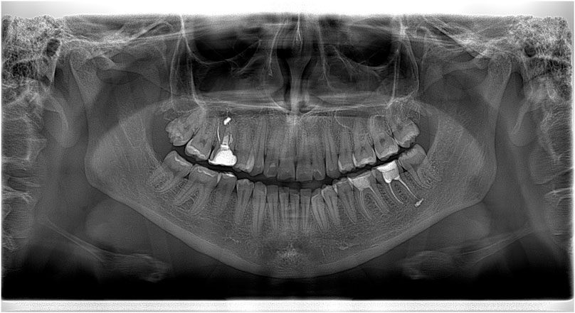
FIGURE 1. Large size image produced by the Morita system.

Then, the acquired images can be exploited in a different manner. First, they can be saved in a clinic depository and/or passed to a doctor and/or to a patient. Saving in a depository is desired since a patient or a doctor might need this image later or for some other purposes. Passing to a patient can be done because the patient might go to another clinic or another doctor. In both cases, image lossy compression is possible and even sometimes needed (if a great number of images are obtained in a laboratory or clinic). However, it should be visually lossless compression and no visible distortions should be seen (detectable) in any part of an image of a large size. Note that lossy compression can be also desired if communication lines have a limited bandwidth, a user or a clinic pays for Internet traffic, etc.

Although acquired images or their fragments under interest can be visualized on screens of very different devices, it is recommended and common to use laptops and stationary computers (monitors) with large sizes and appropriate quality screens. Note also that doctors can look at and analyze images in different scales using the maximal resolution scale for image fragments under interest. Because of its large size, a dental image has to be scrolled for analysis in maximal resolution scale to see the smallest details.

Since it is possible to expect that the monitor type has an impact on image perception, good screens are mainly used for visualization and analysis of an image in aggregate or its parts. In our study, the evaluators used the following monitors: (a) a monitor of laptop ASUS (15.6″, 1920 × 1080, Full HD, IPS), (b) an HP monitor (with a diagonal 27.1″, 1920 × 1080, Full HD, IPS), (c) a monitor of IPad (diagonal 10.2″, 2160 × 1620, IPS). Since distortions due to lossy compression appear themselves more for the maximal resolution scale, the doctors evaluated the images visually using the maximum zooming of images for the aforementioned monitors. Then, we need to provide visually lossless compression for the maximal resolution scale for fragments of the size of a few hundred to a few hundred pixels. Keeping this in mind, we have to carry out analysis correspondingly, i.e., for image fragments. We have chosen their size to be 512 × 512 pixels since it is convenient for DCT-based coders. In addition, such size fragments can be easily and conveniently placed nearby to each other for comparing the original and compressed versions according to recommendations in Testolina et al. (2021). Examples of such fragments taken from the image in Figure 1 are presented in Figure 2.

FIGURE 2

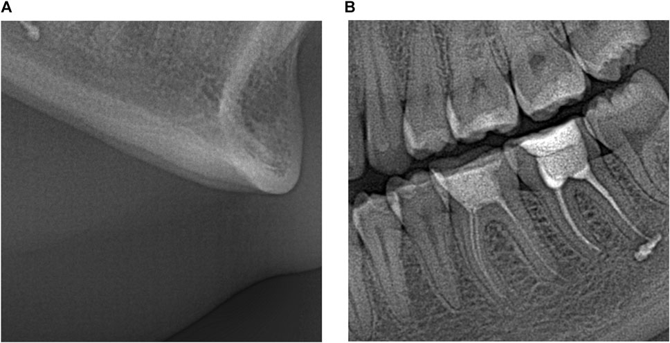
FIGURE 2. 512 × 512 pixel fragments of different complexity taken from large size image in (A,B).

As it is seen, image fragments can be of different complexity where the fragment in Figure 2B contains more details, edges, and textures compared to a rather simple image fragment in Figure 2A. Besides, noise can be easily noticed in the latter image, especially in homogeneous areas having medium intensity. This is not surprising because of the following reasons. First, for the safety of patients, X-ray images are low dose and this leads to the presence of quite intensive noise (Lee et al., 2018). Second, noise is signal-dependent (Lee et al., 2018; Abramova et al., 2020) and this explains why the noise is better seen in homogeneous image regions having a larger local mean. Third, the noise is spatially correlated (Abramova et al., 2020) and this is one reason why noise is visible—spatially correlated noise is more visible than white noise of the same intensity. Meanwhile, noise characteristics also depend on the imaging mode (Abramova et al., 2020). The most adequate model of the noise occurred to be ${\widehat{\sigma }}^2={\widehat{\sigma }}_{\mu }^2\bullet I_{ij}^2+\widehat{k}\bullet I_{ij}+{\widehat{\sigma }}_a^2$ where ${\widehat{\sigma }}_{\mu }^2$ and ${\widehat{\sigma }}_a^2$ are the estimates of multiplicative and additive noise variances, respectively, $\widehat{k}$ is the estimate of the quasi-Poissonian component parameter, and $I_{ij}$ denotes image true value in the ij-th pixel. Then, for a given fragment, equivalent variance can be estimated as

${\widehat{\sigma }}_{eq}^2={\widehat{\sigma }}_a^2+{\widehat{\sigma }}_{\mu }^2{\displaystyle {\sum }_{i=1}^N}{\displaystyle {\sum }_{j=1}^M}{I}_{ij}^2/NM+\widehat{k}{\displaystyle {\sum }_{i=1}^N}{\displaystyle {\sum }_{j=1}^M}{I}_{ij}/NM(1)$

where N and M in Eq. 1 define the fragment size. Then, for one mode of the Morita system operation, ${\widehat{\sigma }}_{eq}^2$ varies from about 10 to 60 depending on fragment mean intensity. For the second mode, ${\widehat{\sigma }}_{eq}^2$ varies from 30 to almost 200 (for the fragment in Figure 2B) (Krivenko et al., 2020). In any case, the noise occurs to be visible.

Meanwhile, for images acquired by the Dentsply Sirona system, the noise is hardly noticed.

2.2 Providing visually lossless compression by setting the fixed PCC

2.2.1 Used metrics and considered coders

Recall that for a visually lossless approach we need some adequate visual quality metric and the corresponding distortion invisibility threshold. Metric adequateness for a given type of distortion is usually determined by analysis of the Spearman rank order correlation coefficient (SROCC) between metric values and mean opinion score (MOS) for image databases that contain images with the considered type of distortions. The image database TID 2013 (Ponomarenko et al., 2015b) is a good option that contains images distorted by lossy compression. It has been established that, for many metrics including PSNR, SROCC exceeds 0.9, i.e., distortions due to lossy compression are quite adequately characterized. Meanwhile, there are several metrics for which SROCC is between 0.96 and 0.97 including PSNR-HVS-M (Ponomarenko et al.), feature similarity (FSIM) index (Zhang et al., 2011), mean deviation similarity index (MDSI) (Ziaei Nafchi et al., 2016), Haar wavelet-based perceptual similarity index (HaarPSI) (Reisenhofer et al., 2018), and some others (Wang et al., 2004). For some of them, the invisibility threshold has been determined. For example, for PSNR-HVS-M, the threshold is T_PHVSM ≈ 40 dB (Ponomarenko et al., 2015a). In turn, for MDSI the threshold is T_MDSI ≈ 0.22 (Li et al., 2022). So, let us rely on the metric PSNR-HVS-M expressed for 8-bit images as

${PSNR-HVS-M}^n=10{\mathit{log}}_{10}\left(\frac{{255}^2}{{MSE-HVS-M}^n}\right),(2)$

where MSE-HVS-Mⁿ in Eq. 2 is calculated in 8 × 8 blocks in the DCT domain taking into consideration two peculiarities of the human vision system (HVS)—the lower sensitivity of HVS to distortions in high spatial frequencies than distortions in low spatial frequencies and masking effect. Similarly to PSNR, PSNR-HVS-M is expressed in dB and its larger values relate to better visual quality. For additive white Gaussian noise and similar distortions, PSNR-HVS-M occurs to be slightly larger than the corresponding PSNR due to the masking effect. This property can indirectly describe the properties of distortions introduced by image lossy compression (Abramova et al., 2023).

In this paper, we consider four DCT-based coders. One of them is JPEG controlled by quality factor (QF). Smaller QF values are associated with larger CR and greater introduced distortions.

ADCTC (Ponomarenko et al., 2007) employs a partition scheme to adapt to image content and uses rectangular shape blocks where all sizes of block sides are powers of two to ensure the possibility of using fast DCT algorithms. The coder is not fast since partition scheme optimization needs some time, the decompression is faster than compression.

The AGU-M coder uses 32 × 32 pixel blocks and an advanced algorithm of bit-plane coding of quantized DCT coefficients. In opposition to the standard AGU (https://ponomarenko.info/#dow), AGU-M employs different quantization steps for different spatial frequencies and uses scaling factor (SF, analog of QS) as PCC. The larger SF results in larger CR and greater distortions introduced.

The better portable graphics (BPG) encoder is a part of the HEVC video coder and it has several advantages. In particular, the BPG encoder provides higher CR compared to JPEG and many other methods for the same quality characterized by PSNR. Its available versions can operate with data from 8 to 14 bits per channel. Here, we present the results obtained for the grayscale BPG version 0.9.8 offered at https://bellard.org/bpg/. The parameter Q (that can be only integer and varies from 1 to 51) plays the role of PCC. Its larger values correspond to a larger CR and greater distortions.

Figure 3 allows comparing the coders’ performance for one fragment of the dental image. Dependencies for all coders are given as functions of CR to offer an opportunity to compare the results (recall that the coders have different PCCs).

FIGURE 3

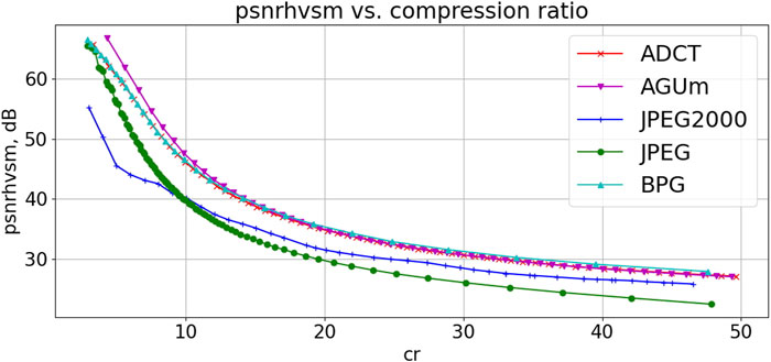
FIGURE 3. Dependences PSNR-HVS-M(CR) for a fragment of dental image in Figure 1.

Analysis of data in Figure 3 shows the following tendencies. AGU-M coder produces the best results in the area of interest (CR=10–15, PSNR-HVS-M>40 dB). The ADCT and BPG encoders perform closely to AGU-M. JPEG and JPRG2000 produce significantly worse results. Thus, the plots in Figure 3 explain one more time why we have paid attention to the analysis of the ADCT, BPG, and AGU-M in our previous and current studies. Similarly, according to PSNR, ADCTC is the best for small CR whilst the BPG encoder is the best for large CR. AGU-M produces results similar to the ADCT and BPG coders. JPEG and JPEG2000 perform considerably worse, especially in the area of interest (CR=10–20, PSNR>35 dB for the three best coders).

2.2.2 The use of fixed PCC for DCT-based coders

Different reasoning can be put into the basis of setting some fixed PCC for DCT-based coders for the considered application. Let us start our analysis for the standard JPEG. It is sometimes supposed that setting QF = 75 practically guarantees that distortions are invisible (Bondžulić et al., 2023). We have applied JPEG with QF = 75 to 20 fragments of the size 512 × 512 pixels taken from the image in Figure 1. It occurred that the minimal and maximal CRs are equal to 5.45 and 11.37, respectively. Minimal and maximal PSNR-HVS-M values are 45.26 dB and 50.65 dB, respectively, i.e., the difference is about 5 dB. Note that the largest PSNR-HVS-M is observed just for the fragment having the smallest CR. These data show that QF can be smaller since there is a reserve for decreasing the PSNR-HVS-M values.

To see what QF can be set, we have calculated the mean PSNR-HVS-M for 20 fragments of Morita images compressed by JPEG with different QF. It follows that mean PSNR-HVS-M equals 40 dB for QF about 49. However, in this case, there are fragments having PSNR-HVS-M smaller and larger than 40 dB (approximate threshold of distortion invisibility). Assuming that PSNR-HVS-M can differ from its mean values by ±2.5 dB, we should set such QF that provides mean PSNR-HVS-M equal to 42.5 dB. This takes place for QF = 60.

Thus, we set QF = 60 and determined CR and PSNR-HVS-M values. The CR values vary from 6.8 to 19.7, PSNR-HVS-M values vary from 41.2 dB to 44.8 dB. This means that by setting QF = 60 the requirement to have invisible distortions for JPEG is satisfied.

A similar analysis has been done for three other coders. For ADCTC it was recommended to set QS = 12 (Krivenko et al., 2020). In this case, for the same set of 20 image fragments, the mean PSNR-HVS-M was the same as above (42.5 dB) where PSNR-HVS-M varied in the limits from 40.5 dB to 45.6 dB (i.e., in slightly larger interval than for JPEG, this is a drawback) and CR varied from 7.5 to 20.6 (i.e., CR values are larger than for JPEG, this is an advantage).

For the AGU-M coder, we recommended setting SF = 8.8 to have the same mean PSNR-HVS-M (Krylova et al., 2021). Then, PSNR-HVS-M was in the limits from 41.1 dB to 45.1 dB (this result is better than for ADCTC) whilst CR varied from 9.4 to 35.0 (both minimal and maximal values are larger than the corresponding values in the previous cases).

Finally, for the BPG encoder, the results are the following (Kryvenko et al., 2022). It was recommended to set Q = 28 (analysis of several dependencies for particular image fragments presented in Figure 4 shows that this is a correct decision). This led to PSNR-HVS-M within the limits from 41.8 dB to 45.9 whilst CR varies from 8.6 to 16.2. This is slightly worse than for the AGU-M coder.

FIGURE 4

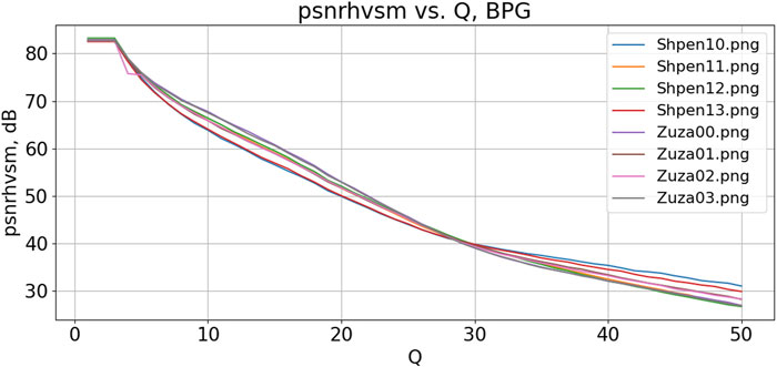
FIGURE 4. Dependencies of PSNR-HVS-M on Q for the BPG encoder for eight image fragments.

Note that, since Q for the BPG encoder can be only an integer and Q increasing by unity leads to PSNR-HVS-M reduction by about 1.5 dB, it is difficult to compare the obtained results to the corresponding results for other coders. Because of this, here we also present the results for Q = 29. PSNR-HVS-M varies within the limits from 40.3 dB to 44.4 dB, CR is from 9.5 to 18.2, i.e., CR has improved by the expense of a lower visual quality and the performance is at approximately the same level as for the ADCTC.

Above, we have considered approaches to lossy compression based on the fixed setting of PCC for the DCT-based coders. Let us denote them as JPEG-FS, ADCTC-FS, AGU-M-FS, and BPG-FS, respectively. A common advantage is that no decompression is used and, thus, the compression procedures are relatively fast (except the ADCT coder for which partition scheme optimization takes significant time). Meanwhile, one general conclusion that follows from the presented results is that, for the fixed PCC, the PSNR-HVS-M values vary in some limits and this opens a certain room for further improvement.

In particular, in the paper (Kryvenko et al., 2022), it was proposed to use the following procedure - apply compression with Q = 28 at the first step and determine PSNR-HVS-M₁ after decompression. If PSNR-HVS-M₁ is within the limits from 41.75 dB to 43.25 dB, leave the compression result. If PSNR-HVS-M₁ is outside these limits, then calculate Q as Q = 28 + [(PSNR-HVS-M₁ – 42.5)/1.5] where [ ] denotes rounding to the nearest integer. This provides a mean PSNR-HVS-M of about 42.5 dB and narrower limits of its variation after the final step. Similar procedures called two-step can be realized for other coders. They are considered in the next section.

3 Results

3.1 Two-step providing of appropriate visual quality

The basic idea of the two-step procedures (Li, 2022; Li et al., 2022) is the following. For a rather small interval for PCC variation, dependencies of PSNR-HVS-M on PCC are almost linear and they are “almost parallel” to each other for particular images. This is seen well in Figure 4 for the BPG coder if Q is in the interval under interest (Q from 25 to 33). Then, knowing a metric value for a given PCC and having some estimate of the derivative of the corresponding rate-distortion curve, it becomes possible to find a PCC that approximately corresponds to the desired value of the considered metric Metr_des.

More in detail, suppose that, in advance (off-line), the average rate-distortion curve Metr_av (PCC) has been obtained. Then, it can be used for two purposes: first—to determine PCC₁, for which Metr_av (PCC) ≈ Metr_des, and, second, to determine $M^{\prime }$ = dMetr_av/dPCC. The first step is to compress an image using PCC₁, to decompress it and to determine Metr₁. This value can be smaller or larger than Metr_des and, knowing $M^{\prime }$, it is possible to calculate PCC₂ as

${PCC}_2={PCC}_1+\left({Metr}_{des}-{Metr}_1\right)/M^{\prime }.(3)$

Note that, in Eq. 3, ${Metr}_{av}$ is often used instead of ${Metr}_1$ (Li et al., 2020a). These two values are the same if PCC can fall into any value. However, for the JPEG and BPG coders, PCC values can be only integer and, thus, PCC₁ can be only integer too. Then, the expression (Suetens, 2017) is more general.

Then, assuming the Gaussian distribution of residual errors of providing Metr_des after the second step, we can set ${Metr}_{des}\approx {Metr}_{thr}+3{\sigma }_M$ where ${\sigma }_M$ is the standard deviation of residual errors for the two-step method. ${\sigma }_M$ depends on the following main factors—a metric used and its desired value and a coder considered. For the metric PSNR-HVS-M, the corresponding studies have been carried out for the ADCT (Li et al., 2020a) and BPG (Li et al., 2020b) coders. For ADCTC for PSNR-HVS-M_des about 40 dB, ${\sigma }_M\approx 0.55dB$ for highly textured images and smaller for simpler structure ones. So, we can set PSNR-HVS-M_des = 41.65 dB for the two-step procedure. For the BPG encoder, ${\sigma }_M\approx 0.6dB$ and, thus, it is reasonable to set PSNR-HVS-M_des = 41.8 dB. Note that in both cases, PSNR-HVS-M_des is smaller than the average PSNR-HVS-M (42.5 dB) we provided for the PCC fixed setting (see previous Section).

The advantages of the two-step approach are that it usually provides minimal PSNR-HVS-M larger than for the case of the fixed PCC setting and maximal PSNR-HVS-M smaller than for the fixed PCC setting. In the first case, this results in smaller probability that distortions are visible. In the second case, a larger CR is provided.

We have not carried out experiments for JPEG and AGU-M coders intended to determine ${\sigma }_M$ for them for different PCCs. However, taking into account the limits of variation of PSNR-HVS-M for the fixed PCC for average PSNR-HVS-M equal to 42.5 dB reported in the previous Section, it is possible to set PSNR-HVS-M_des = 41.65 dB for both JPEG and AGU-M. We have also checked if this setting is correct by calculating the residual errors in experiments with the set of dental image fragments.

Let us start with the results for the AGU-M coder. For the two-step procedure, SF at the second step is from 8.4 to 11.7, the minimal PSNR-HVS-N has occurred to be equal to 41.4 dB whilst the maximal is of about 41.8 dB. This means that the variations of image visual quality according to the metric PSNR-HVS-M are very small. CR values are from 11.1 to 38.3, i.e., minimal and maximal CRs are better than for any other approach considered above.

For the BPG-encoder, the final values of Q are from 26 to 30, the minimal and maximal PSNR-HVS-M are from 41.8 dB to 43.3 dB (i.e., the interval is larger than for AGU-M), and CRs are in the limits from 9.9 to 19.3. In other words, the results are more stable than for the fixed Q according to PSNR-HVS-M and slightly better according to CR.

The compression parameters for the ADCT coder are the following. QS at the second step varies in the limits from 11.0 to 16.3, PSNR-HVS-M is in the limits from 41.3 dB to 41.8 dB, and minimal and maximal CRs are equal to 8.3 and 28.9. Totally, the results are at the same level as for the BPG encoder and worse than for the AGU-M coder.

Finally, for JPEG, QF is from 47 to 61, PSNR-HVS-M is in the limits from 41.3 dB to 41.7 dB and CR varies from 7.9 to 20.4. This is, in general, worse than for all coders considered above. According to the case of fixed QF setting (see Section 3), there is a small benefit in CR values.

Summarizing the results of the two-step procedure, we can state that it provides more stable values of PSNR-HVS-M (they are very close to the desired PSNR-HVS-M) and larger values of minimal and maximal CR. The payment for these improvements is an increase in computations since more time is spent on image compression, decompression, and final compression at the second step.

3.2 JPEG-compression based on JND

Let us first recall some results presented in the papers (Bondžulić et al., 2021; Bondžulić et al., 2023; Testolina et al., 2023). In Bondžulić et al. (2023), analysis of QF values for the first JND point (JNDP1) has been carried out for two image databases specially designed for this purpose, MCL-JCI and JND-Pano (panoramic images). Although color image compression has been studied, the obtained results seem valuable for our case. It has been shown that PSNR for JNDP1 varies in very large limits—from 27.6 to 46.0 dB for the MCL-JCI database and from 20.9 to 44.7 dB for the JND-Pano database. QF varies from 25 to 70 and from 38 to 75, respectively. This shows that the adequateness of PSNR and distortion invisibility threshold for it [about 36 dB according to Ponomarenko et al. (2015a)] is of doubt. In turn, PSNR-HVS-M for JNDP1 varies from 36.2 to 48.1 dB for the MCL-JCI database and from 39.9 to 49.2 dB for the JND-Pano database. Thus, PSNR-HVS-M is more adequate in characterizing visual quality (its limits of variation are considerably narrower than for PSNR) although PSNR-HVS-M and its invisibility threshold are not perfect.

In Ponomarenko et al. (2020) it has been also shown that, for noisy images, the difference between the same image contaminated by the noise of different intensities, becomes visible if intensities differ by 10%–20%. Then, since we have equivalent variances from 10 to 200 (see Section 2.1), the MSE of distortions introduced by lossy compression should be from 1 to 20. For images compressed with MSE = 1, distortions are not seen, they start to be visible for MSE ≈ 3 in the worst case. Thus, the PSNR of noisy images compressed in a visually lossless manner can be from approximately 35 dB–43 dB depending on the noise intensity. These results are in good agreement with the results reported above for both databases.

There are approaches to the prediction of QF for JNDP1 (Lin et al., 2020; Stojanovic et al., 2022). The method (Stojanovic et al., 2022) is based on exploiting a simple parameter called mean gradient magnitude (MGM) able to characterize an image to be compressed. It is shown that the RMSE of such a prediction (PSNR is predicted for JNDP1 based on MGM) is about 1 dB. MGM can be defined as:

$MGM=\frac{1}{NM}{\displaystyle {\sum }_{\forall n,m}}\frac{1}{g_{\mathit{max}}}\sqrt{g_x^2\left(n,m\right)+g_y^2\left(n,m\right),}(4)$

where g_max in Eq. 4 is the maximum magnitude value, g_max = 4.472 for grayscale images with a dynamic range from 0 to 1.

MGM values are in the limits from 0 to 0.17 although they mainly concentrate in the limits from 0.01 to 0.07. For smaller MGM that corresponds to simpler structure images without noise, PSNRs for JNDP1 are larger. Whilst, for MGM ≈ 0.07, PSNRs for JNDP1 are of about 32 dB, they are of about 42 dB for MGM ≈ 0.01. The formula for PSNR prediction obtained in Bondžulić et al. (2021) is the following:

$PSNR=\left\{\begin{array}{c}2115.5{MGM}^2-377MGM+46.4,MGM\le 0.0896\\ 29.58,MGM>0.0896\end{array}\right.,(5)$

where for MGM = 0.0896 the mapping function in Eq. 5 reaches its minimum value equal to PSNR_min = 29.58 dB.

We have decided to calculate MGM for our 512 × 512 fragments of Morita images. The MGM values are from 0.031 to 0.071. Then, PSNR values for JNDP1 should be from 30 dB to 35.5 dB. For each considered image fragment, a desired PSNR can be provided by the two-step procedure. For 4 out of 20 test fragments, the difference between the desired PSNR (recommended by Eq. 5) and PSNR provided by the two-step procedure exceeded 1 dB—the maximal difference was equal to 1.3 dB. Then, we have also calculated CR and PSNR-HVS-M. CR has varied in the limits from 6.4 to 20.3, i.e., approximately in the same limits as for approaches considered above. However, problems have arisen with QF and PSNR-HVS-M of compressed images. QF varied from 16 to 84. PSNR corresponding to small QF was about 30 dB, which, according to our experience, is too small. This is confirmed by image fragments in Figure 5 where original (Figure 5A) image and the corresponding compressed one (Figure 5B) are represented. Distortions (mainly, blocking artifacts) are seen in compressed image. Thus, we do not deal with the desired visually lossless compression.

FIGURE 5

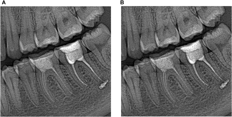
FIGURE 5. Original (A) and compressed (B) versions of image fragments.

Meanwhile, there are also fragments that have been compressed with PSNR in the limits from 38 dB to 42 dB and PSNR-HVS-M from 44.5 dB to 49.5 dB. For them, no distortions are visible and the recommended QFs exceed 70. According to previous experience (see Section 3), smaller QF values can be used while keeping the introduced distortions invisible.

Thus, we can state that the approach based on JNDP1 prediction does not perform satisfactorily and, at the moment, cannot be recommended for practical use. To our opinion, there are several reasons behind this imperfection. First, there are several factors that lead to errors in setting QF. They are imperfect dependence of PSNR for JNDP1 on MGM where some points differ from the fitted curve by a few dB and the limited accuracy of the two-step approach that provides the desired PSNR with errors exceeding 1 dB. Second, the fitted curve (Prince and Links, 2006) has been obtained for color images without noise and we have used it for grayscale noisy images. Recall here that PSNR of about 30 dB corresponds to MSE of introduced losses of about 65 (for 8-bit images that we have in our experiments). This means that MSE is comparable to noise intensity and, thus, it is not surprising that the introduced losses are visible.

The obtained results do not mean that the approach based on JNDP1 has no potential for the considered application. However, the dependence of PSNR (or PSMR-HVS-M) on one parameter or parameters describing image characteristics has to be additionally studied and made more accurate.

3.3 Visually lossless compression of almost noise-free images

As it has been mentioned above, some X-ray imagers produce almost noise-free images. Example of such images having large sizes is given in Figure 6. As one can see, noise is not visible.

FIGURE 6

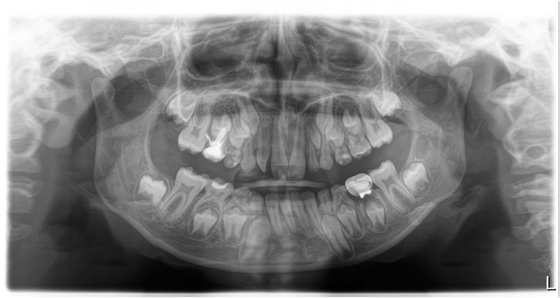
FIGURE 6. Example of large size dental images produced by the Imager Dentsly Sirona (https://www.dentsplysirona.com/en/discover/discover-by-brand/orthophos-e.html).

We have briefly analyzed the rate-distortion characteristics for fifteen 512 × 512 fragments of almost noise-free images. The goal for this was to analyze do they differ a lot from the dependencies earlier obtained for image fragments considered above. Since for all approaches we need average rate-distortion curves, let us obtain them and compare them to the previously used ones. Figure 7 presents the average dependence of PSNR-HVS-M on QF for JPEG. It is monotonous and almost linear in the area of interest. The derivative dPSNR-HVS-M/dQF is practically the same as for the Morita image fragments—about 0.22. This means that, if we would like to provide an average PSNR-HVS-M equal to 42.5 dB for fixed QF, we can set QF = 55 (for the considered type of dental images).

FIGURE 7

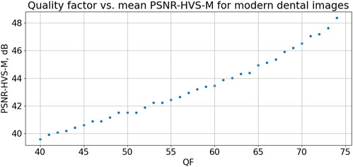
FIGURE 7. Dependence of mean PSNR-HVS-M on QF for JPEG for fragments for almost noise-free dental images.

Let us see, what are the provided compression characteristics in this case. PSNR-HVS-M values are from 41.9 dB to 42.8 dB, i.e., in rather narrow interval. CR values are from 14.2 to 24.6, i.e., both minimal and maximal CRs are larger than the corresponding ones for the Morita image fragments.

In turn, Figure 8 represents the dependence of PSNR-HVS-M on SF for the AGU-M coder. Similarly to the dependences in Figure 4, it is monotonous. The values of average PSNR-HVS-M are slightly larger than for Morita image fragments. If one would like to set a fixed SF for providing average PSNR-HVS-M about 42.5 dB, then SF=9.93. Setting this SF leads to the following results: PSNR-HVS-M varies in the limits from 41.9 dB to 42.9 dB, i.e., in a narrow range, CR is in the limits from 22.8 to 52.5, i.e., the CR values are considerably better than for Morita system image fragments. We associate this with the practical absence of noise. The CR values are also considerably better (larger) than for the JPEG data given above.

FIGURE 8

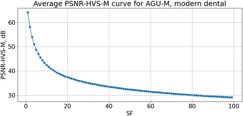
FIGURE 8. Dependence of mean PSNR-HVS-M on SF for AGU-M for fragments for almost noise-free dental images.

Figure 9 presents the average dependence of PSNR-HVS-M on QS for the ADCT coder. According to this curve, one has to set QS = 11.98 to provide the average PSNR-HVS-M equal to 42.5 dB. For this QS used as the fixed setting, the results are the following. PSNR-HVS-M varies from 41.8 dB to 43.2 dB, i.e., in quite narrow (appropriate) limits. CR is from 21.4 to 59.2, i.e., they are comparable to the interval of CR variation for the AGU-M coder.

FIGURE 9

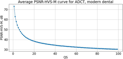
FIGURE 9. Dependence of mean PSNR-HVS-M on QS for ADCTC for fragments for almost noise-free dental images.

Finally, we have checked the results for the BPG encoder. According to the average curve, Q was set equal to 27 to ensure the average PSNR-HVS-M of about 42.5 dB. As the results, PSNR-HVS-M values vary from 41.9 dB to 43.0 dB (in appropriately narrow intervals) and CRs are from 22.4 to 71.6. This means that, for more complex structure images, CR is approximately the same as for AGU-M and ADCT coders whilst, for simple structure images, there is a certain benefit in CR provided by the BPG coder.

Let us summarize the results given above in this Section. First, we have checked whether distortions are visible for some fragments compressed by all four coders providing the average PSNR-HVS-M = 42.5 dB and have not found such cases. Second, it has been established that for the fixed values of PCC, the differences in PSNR-HVS-M values for particular fragments do not differ a lot (the variation interval widths are about 1 dB). Then, it is possible to expect that the 2-step procedure is able to provide even narrower variation intervals. Thus, for the 2-step procedure, we have decided to set the desired PSNR-HVS-M equal to 42 dB and to check what results can be obtained in this case for all four coders.

For JPEG, the obtained results are the following. The provided PSNR-HVS-M varies from 41.6 dB to 42.1 dB, QF values are mostly equal to 52 although there are a few images for which QF equals either 51 or 53. The provided CR is from 17.1 to 25.5. The positive feature is that the variation range for PSNR-HVS-M has decreased. CR values have slightly increased whilst the mean PSNR-HVS-M has decreased which can be expected. Taking into account that the two-step procedure requires two compressions and one decompression, we do not see an essential difference between applying the fixed (properly set) QF or using the two-step procedure for JPEG.

For the AGU-M coder, PSNR-HVS-M varies from 41.96 dB to 42.04 dB, i.e., very high accuracy is provided. SF is from 9.8 to 11.0, i.e., SF adaptation to image properties takes place. Finally, CR values are from 23.3 to 58.5, i.e., they are considerably better than for JPEG and slightly better than for the case of setting fixed SF for the AGU-M coder (see the corresponding data above).

The coder ADCT has produced similar results. PSNR-HVS-M is in the limits from 41.97 dB to 42.08 dB, i.e., the desired PSNR-HVS-M is provided with high accuracy. This is due to the adaptation of QS to image content—QS varies from 11.8 to 13.5. CR values are from 22.7 to 63.2, i.e., the minimal CR is slightly less and the maximal CR is greater than for the AGU-M coder.

Finally, the BPG coder produces PSNR-HVS-M in the limits from 41.9 dB to 42.9 dB. As one can see, the provided mean PSNR-HVS-M is slightly larger than the desired one. This results from the fact that Q can be only integer. The Q values for almost all image fragments are equal to 27. CR values are from 22.5 to 58.7, i.e., practically the same as for the AGU-M coder. No improvement compared to the fixed setting of Q is offered. This is explained by two reasons. First, the BPG coder produces quite close values of PSNR-HVS-M for fixed Q that differ from each other by about 1–1.2 dB, at least, if the desired PSNR-HVS-M are in the range of interest (40–44 dB). Changing of Q by 1 leads to PSNR-HVS-M changing by about 1.5–1.7 dB, i.e., by more than the aforementioned range width. This means that the two-step procedure produces a limited improvement of accuracy for the considered situation and it is not worth employing it for the BPG coder.

Summarizing the obtained results, we can state that the use of the two-step procedure for providing the desired PSNR-HVS-M offers some benefits for the coders AGU-M and ADCT since the desired PSNR-HVS-M can be provided with higher accuracy and this leads to a certain increase in CR. Meanwhile, there are no obvious reasons to apply the two-step procedure for JPEG and BPG encoders since the accuracy of providing the desired PSNR-HVS-M for them does not improve a lot because of setting PCCs as only integer values.

We have also tested the approach based on MGM calculation, PSNR prediction and its providing by the two-step method. MGM values are smaller than for image fragments with visible noise considered in Sections 3, 4, they are in the limits from 0.012 to 0.026. Then, the predicted PSNRs for JNDP1 are larger—from 38.1 dB to 42.0 dB. They have been provided by the two-step procedure with errors not exceeding 1 dB. As a result, CRs are from 23 to 37 (good results), but PSNR-HVS-M are within the limits from 35.7 dB to 38.7 dB, i.e., below the distortion visibility threshold. Then, we have checked the compressed image fragments. It has occurred that for many of them the introduced distortions are visible.

Figure 10 shows the fragment obtained after visually lossless compression using the two-step procedure for the four considered coders (further denoted as JPEG2st, AGU-M2st, ADCT2st, and BPG2st, respectively). As one can see, it is difficult to find differences between the compressed images (maybe, the image compressed by ADCTC is slightly sharper). There is practically no difference compared to the original image.

FIGURE 10

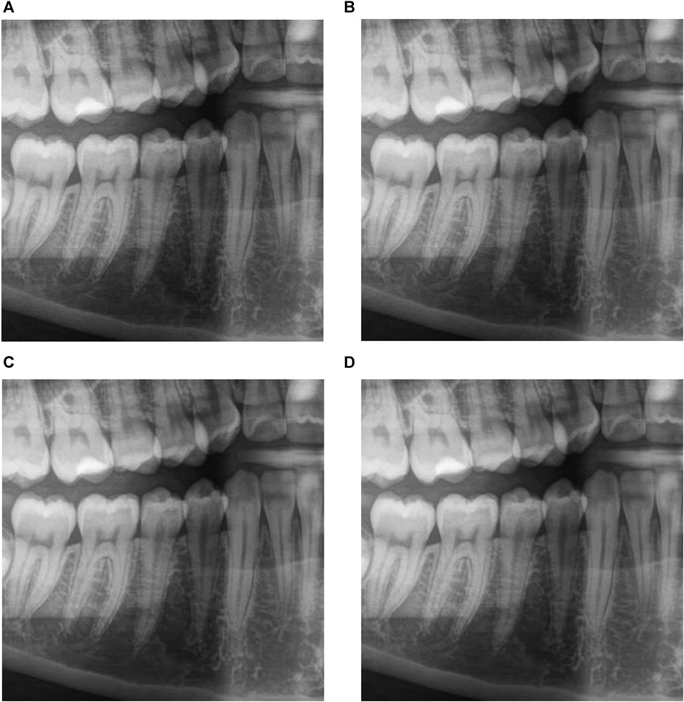
FIGURE 10. The fragment obtained after visually lossless compression using the two-step procedure for JPEG, CR = 14.7, PSNR-HVS-M = 41.97 dB (A), AGU-M, CR = 23.5, PSNR-HVS-M = 42.00 dB (B), ADCT, CR = 23.2, PSNR-HVS-M = 42.00 dB (C) and BPG, CR = 26.3, PSNR-HVS-M = 41.37 dB (D) coders.

Comparing the results presented in this Section for almost noise-free images to the results for noisy images in the previous two Sections, the following two conclusions can be drawn. First, average rate-distortion curves differ a little. Average values of PSNR-HVS-M for the same PCC for almost noise-free images are slightly larger for noise-free images (this difference does not lead to any problem if the two-step procedure is applied). Second, on average, larger final values of CR are obtained for noise-free images—this is not surprising, see the results presented in Krivenko et al. (2018).

Above, in the design of visually lossless compression of dental images and comparison of performance characteristics for different coders, we have relied on the following. First, the results on the distortion visibility threshold presented for images in the database TID2013 (Ponomarenko et al., 2015a) have been taken into account. Second, we have taken into account the results of verification experiments earlier carried out for the ADCT, AGU-M, and BPG coders with the fixed PCCs described in our papers (Krivenko et al., 2020; Krylova et al., 2021; Kryvenko et al., 2022). However, the threshold of distortion invisibility according to the PSNR-HVS-M metric is approximate and this has been confirmed by experiments in Bondžulić et al. (2021). Thus, we need to be sure that the proposed approaches to visually lossy compression do not lead to a reduction of the diagnostic value of compressed images.

4 Discussion

We have carried out experiments with compressed image fragments to understand the following: 1) how often a specialist (dentist) sees the differences between original and compressed image fragments; 2) do these differences have an impact on the diagnostic value of compressed images; 3) do the results for the considered coders differ between each other. Preparing this experiment, we have taken into account the recommendations for performing such experiments and previous experience. First, an observer’s distance to the monitor has to be fixed and it should be convenient for a particular observer. Second, it is usually enough to have about 15 s to decide if there are differences in the viewed images and if are there artifacts in the compressed image (that, in our case, influence its diagnostic value). Third, the experiment should not be too long since an observer becomes tired and starts to perform his/her task improperly. Fourth, between pairs of images following each other in comparison, there should be a small break (dark screen) “to remove the previous pair from human memory.”

Thus, each pair of image fragments was shown for comparison for 5–20 s and an observer had to press either the button “Identical” or the button “Different.” In the latter case, the observer had to press either the button “Appropriate” or the button “Inappropriate” where the latter means that the distortions introduced by lossy compression have led to lost diagnostic information. Between the subsequent pairs, 5-s break with the dark screen was offered. Each observer has been given 50 pairs of image fragments to be compared. As a result, the experiment did not last more than 25 min (in fact, no one experiment lasted more than 22 min with an average duration of 16 min). The fragments have been randomly chosen from the considered large-size images in advance, compressed, and saved in the folder used in the experiments. This was done since the compression and decompression time could be larger than the time taken for comparison of each pair of image fragments. Note that compression and decompression time depends on several factors including the coder used (the largest compression/decompression time is for the ADCT coder), computer characteristics, and software realization of a given coder.

The original image fragment was always placed left with respect to the corresponding compressed fragment. The buttons were put below the visualized image fragments. Taking into account that each of the four doctors carried out 50 comparisons, 200 comparisons have been performed total (for each coder). Thus, the probability that two image fragments are different (P_d) could be determined. No considerable difference in the results for different monitors have been observed. Similarly, no significant difference has been noticed in the results for doctors participating in experiments. Comparisons for different coders (and their variants) were done on different days. The doctors were not told what coder is under study at the current moment. Each doctor participated in experiments carried out on different computers. Monitors have been viewed approximately from the distance 1.6D_v where D_v is the monitor height.

The comparison results for images acquired by the Morita system are presented in Table 1. In addition to P_d, we give the additional data that allow comparing the considered approaches to compression: the range of PSNR-HVS-M values and the range of CR values for the analyzed image fragments. Keeping in mind that P_d is estimated with RMSE about 0.02, the conclusions that can be drawn are the following:

1) The fixed setting of the PCC leads to approximately the same P_d as the two-step approach for a given coder; the difference for them is in narrower ranges of PSNR-HVS-M variation and slightly larger minimal and maximal CR values for the two-step approach;

2) The ADCTC with fixed QS setting and with the use of the two-step procedure produces slightly smaller P_d, a more thorough comparison has shown that object edges are preserved by this coder better than by other considered coders;

3) Wider ranges of CR variation have been observed in experiments compared to the cases analyzed in previous Sections; this can be explained by wider variations of image fragment content (200 fragments have been considered instead of 15–20 analyzed in previous experiments);

4) Slightly larger CR values have been observed for the two-step procedure; the largest values took place for the AGU-M coder although the differences in CR values are not significant.

TABLE 1

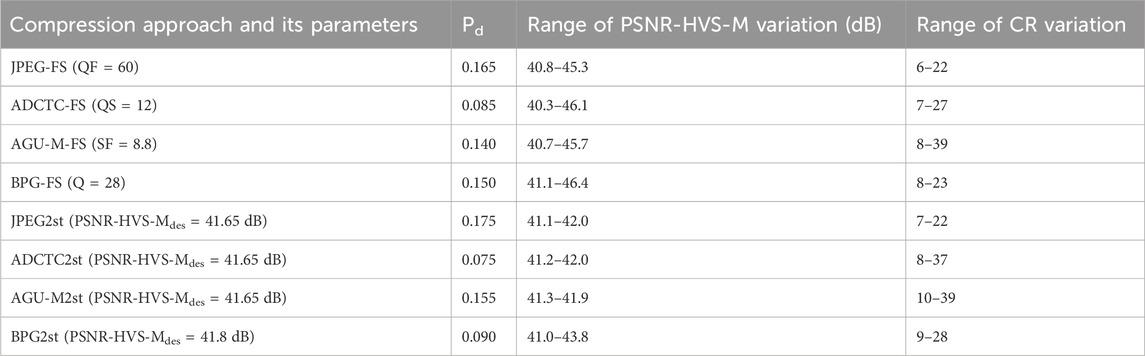
TABLE 1. The obtained experimental data for the Morita imager.

It is rather important to notice that in none of the cases, the quality of compressed images for the methods listed in Table 1 was treated as inappropriate. Meanwhile, we have also tested the compression procedure for JPEG based on JNDP1. For this one, P_d is equal to 0.27, i.e., the difference between original and compressed image fragments has been found considerably more often. Moreover, with probability of 0.08, the compressed images were treated as inappropriate, mainly because of visible blocking effects (artifacts).

Since the results for the fixed setting of PCC and two-step procedure were close to each other, only the two-step procedure has been used in experiments for almost noise-free images. The obtained results are presented in Table 2. The desired PSNR-HVS-M was equal to 42 dB for all considered coders.

TABLE 2

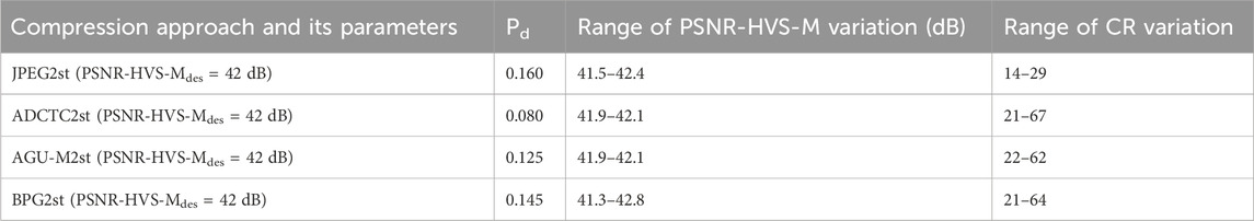
TABLE 2. The obtained experimental data for the Dentsply Sirona imager.

As one can see, the values of P_d are approximately in the same range as in Table 1 where the best result (the smallest P_d) is again provided by the ADCT coder. Besides, the ADCT and AGU-M coders provide the smallest variations of PSNR-HVS-M whilst JPEG and the BPG encoders are characterized by wider variations (since PCC values for them can be only integer). No cases when the quality of compressed images has been considered inappropriate have been detected.

The CR values for three modern coders are significantly larger than for JPEG and they are considerably larger than 10. The CR values are also, in general, considerably larger than the CR values in Table 1 and this can be explained by the fact that images acquired by the Dentsply Sirona system contain less noise.

Thus, we can recommend using PSNR-HVS-M_des = 42 dB and the two-step procedure for providing either visually lossless compression or lossy compression for which introduced distortions can be hardly noticed and do not affect the diagnostic value of dental images acquired by modern systems.

5 Conclusion

The task of visually lossless compression of dental images acquired by two modern systems is considered. The images usually have a large size and, due to this, it is worth applying lossy compression for their transferring via communication lines and storage. Three approaches to visually lossless compression are considered, namely, the use of the fixed PCC, the use of the two-step compression, and the approach based on the first just noticeable distortion point. It is shown by experiments carried out by four qualified dentists for three types of monitors with 200 image fragments used in comparisons that the latter approach is not perfect at the moment and it produces the largest percentage of situations when distortions in compressed image fragments are noticeable and able to negatively affect the diagnostic value of dental images.

For the two former approaches, the compression characteristics depend on whether the noise is visible or not. For images with visible noise, the minimal and maximal values of produced CR are smaller than for the almost noise-free images. Note that in the latter case, the provided CR varies from about 20 to almost 70 for modern coders that significantly outperform JPEG (in the sense of larger CR for approximately the same visual quality and P_d). If one would like to have smaller P_d than in our experiments, it is possible to increase PSNR-HVS-M_des for the two-step approach or to use larger fixed QF for JPEG and smaller fixed values of SF, QS, and Q for AGU-M, ADCT, and BPG coders, respectively. However, smaller minimal and maximal CR values are then produced.

In the future, we plan to consider other modern coders and quality metrics. Images produced by other dental systems can be studied as well. Considering the obtained results, it will be interesting to perform multi-centered research, increase the number of patients and collect data from dental centers with different geographical locations.

Data availability statement

The original contributions presented in the study are included in the article/supplementary material, further inquiries can be directed to the corresponding author.

Ethics statement

The studies involving humans were approved by Ethics committee of Kharkiv National Medical University. The studies were conducted in accordance with the local legislation and institutional requirements. The participants provided their written informed consent to participate in this study. Written informed consent was obtained from the individual(s) for the publication of any potentially identifiable images or data included in this article.

Author contributions

LK: Writing–original draft, Writing–review and editing, Data curation, Software, Supervision, Validation, Visualization, Methodology. OK: Methodology, Software, Validation, Visualization, Writing–review and editing. VL: Conceptualization, Data curation, Investigation, Methodology, Project administration, Software, Writing–original draft, Writing–review and editing. SK: Formal Analysis, Investigation, Methodology, Resources, Software, Validation, Writing–review and editing.

Funding

The authors declare that no financial support was received for the research, authorship, and/or publication of this article.

Conflict of interest

The authors declare that the research was conducted in the absence of any commercial or financial relationships that could be construed as a potential conflict of interest.

Publisher’s note

All claims expressed in this article are solely those of the authors and do not necessarily represent those of their affiliated organizations or those of the publisher, the editors, and the reviewers. Any product that may be evaluated in this article, or claim that may be made by its manufacturer, is not guaranteed or endorsed by the publisher.

References

Abramova, V., Krivenko, S., Lukin, V., and Krylova, O. (2020). “Analysis of noise properties in dental images,” in 2020 IEEE 40th International Conference on Electronics and Nanotechnology (ELNANO), Kyiv, Ukraine (IEEE), 511–515. Available from: https://ieeexplore.ieee.org/document/9088768/ (Accessed October 19, 2020).

CrossRef Full Text | Google Scholar

Abramova, V., Lukin, V., Abramov, S., Kryvenko, S., Lech, P., and Okarma, K. (2023). A fast and accurate prediction of distortions in DCT-based lossy image compression. Electronics 12 (11), 2347. doi:10.3390/electronics12112347

CrossRef Full Text | Google Scholar

Afnan, A., Ullah, F., Yaseen, Y., Lee, J., Jamil, S., and Kwon, O. J. (2023). Subjective assessment of objective image quality metrics range guaranteeing visually lossless compression. Sensors 23 (3), 1297. doi:10.3390/s23031297

PubMed Abstract | CrossRef Full Text | Google Scholar

Al-Shaykh, O. K., and Mersereau, R. M. (1998). Lossy compression of noisy images. IEEE Trans Image Process 7 (12), 1641–1652. doi:10.1109/83.730376

PubMed Abstract | CrossRef Full Text | Google Scholar

Al-Shebani, Q., Premaratne, P., Vial, P. J., and McAndrew, D. J. (2019). The development of a clinically tested visually lossless Image compression system for capsule endoscopy. Signal Process. Image Commun. 76, 135–150. doi:10.1016/j.image.2019.04.008

CrossRef Full Text | Google Scholar

Anthony Seibert, J. (2020). Archiving, chapter 2: medical image data characteristics. Society for imaging informatics in medicine. Available from: https://siim.org/page/archiving_chapter2.

Google Scholar

Baghaie, A., Yu, Z., and D’Souza, R. M. (2015). State-of-the-art in retinal optical coherence tomography image analysis. Quantitative Imaging Med. Surg. 5 (4), 603–617. doi:10.3978/j.issn.2223-4292.2015.07.02

PubMed Abstract | CrossRef Full Text | Google Scholar

Blau, Y., and Michaeli, T. (2019). “Rethinking lossy compression: the rate-distortion-perception tradeoff,” in International Conference on Machine Learning, Long Beach, USA (PMLR), 675–685.

Google Scholar

Bondžulić, B., Lukin, V., Bujaković, D., Li, F., Kryvenko, S., and Pavlović, B. (2023). On visually lossless JPEG image compression in 2023 Zooming Innovation in Consumer Technologies Conference (ZINC), Novi Sad, Serbia (IEEE), 113–118. Available from: https://ieeexplore.ieee.org/document/10174090/ (Accessed September 4, 2023).

Bondžulić, B., Stojanović, N., Petrović, V., Pavlović, B., and Miličević, Z. (2021). Efficient prediction of the first just noticeable difference point for JPEG compressed images. Acta Polytech. Hung. 18 (8), 201–220. doi:10.12700/aph.18.8.2021.8.11

CrossRef Full Text | Google Scholar

BPG Image format (2022). BPG Image format. Available from: https://bellard.org/bpg/ (Accessed May 5, 2022).

Google Scholar

Braunschweig, R., Kaden, I., Schwarzer, J., Sprengel, C., and Klose, K. (2009). Image data compression in diagnostic imaging: international literature review and workflow recommendation. RoFo Fortschritte dem Geb. Rontgenstrahlen Nukl. 181 (7), 629–636. doi:10.1055/s-0028-1109341

PubMed Abstract | CrossRef Full Text | Google Scholar

Christopoulos, C., Skodras, A., and Ebrahimi, T. (2000). The JPEG2000 still image coding system: an overview. IEEE Trans. Consum. Electron 46 (4), 1103–1127. doi:10.1109/30.920468

CrossRef Full Text | Google Scholar

Diagnostic and Imaging Equipment (2020). Diagnostic and imaging equipment | MORITA. Available from: https://www.jmoritaeurope.de/en/products/diagnostic-and-imaging-equipment-overview/ (Accessed October 19, 2020).

Google Scholar

Eraso, F. E., Analoui, M., Watson, A. B., and Rebeschini, R. (2002). Impact of lossy compression on diagnostic accuracy of radiographs for periapical lesions. Oral Surg. Oral Med. Oral Pathology, Oral Radiology, Endodontology 93 (5), 621–625. doi:10.1067/moe.2002.122640

PubMed Abstract | CrossRef Full Text | Google Scholar

M. P. Federle, S. R. Sinha, and P. D. Poullos (2018). Imaging in gastroenterology (Philadelphia, PA: Elsevier).

Google Scholar

Fidler, A., and Likar, B. (2007). What is wrong with compression ratio in lossy image compression? Radiology 245 (1), 299–300. author reply 299-300. doi:10.1148/radiol.2451062005

PubMed Abstract | CrossRef Full Text | Google Scholar

Flint, A. C. (2012). Determining optimal medical image compression: psychometric and image distortion analysis. BMC Med. Imaging 12, 24. doi:10.1186/1471-2342-12-24

PubMed Abstract | CrossRef Full Text | Google Scholar

Flynn, M. J., Hames, S. M., Wilderman, S. J., and Ciarelli, J. J. (1996). Quantum noise in digital X-ray image detectors with optically coupled scintillators. IEEE Trans. Nucl. Sci. 43 (4), 2320–2325. doi:10.1109/23.531897

CrossRef Full Text | Google Scholar

Foos, D. H., Slone, R. M., Whiting, B. R., Kohm, K. S., Young, S. S., Muka, E., et al. (1999). in Dynamic viewing protocols for diagnostic image comparison. Editor E. A. Krupinski (San Diego, CA), 108–120. Available from: http://proceedings.spiedigitallibrary.org/proceeding.aspx?articleid=981183 (Accessed December 18, 2023).

Google Scholar

Fornaini, C., and Rocca, J. P. (2022). Relevance of teledentistry: brief report and future perspectives. Front. Dent. 19, 25. doi:10.18502/fid.v19i25.10596

PubMed Abstract | CrossRef Full Text | Google Scholar

Georgiev, V. T., Karahaliou, A. N., Skiadopoulos, S. G., Arikidis, N. S., Kazantzi, A. D., Panayiotakis, G. S., et al. (2013). Quantitative visually lossless compression ratio determination of JPEG2000 in digitized mammograms. J. Digit. Imaging 26 (3), 427–439. doi:10.1007/s10278-012-9538-7

PubMed Abstract | CrossRef Full Text | Google Scholar

Guy, C., and Ffytche, D. (2005). An introduction to the principles of medical imaging. London : Singapore ; Hackensack, NJ: Imperial College Press ; Distributed by World Scientific Pub, 374. Rev.

Google Scholar

HBC (2023). Dental imaging in the cloud: overcoming data management and storage challenges. Healthc. Bus. Club. Available from: https://healthcarebusinessclub.com/articles/healthcare-provider/technology/dental-imaging-in-the-cloud-overcoming-data-management-and-storage-challenges/ (Accessed September 4, 2023).

Google Scholar

Huda, W., and Abrahams, R. B. (2015). Radiographic techniques, contrast, and noise in X-ray imaging. Am. J. Roentgenol. 204 (2), W126–W131. doi:10.2214/ajr.14.13116

PubMed Abstract | CrossRef Full Text | Google Scholar

Jayachandran, S. (2017). Digital imaging in dentistry: a review. Contemp. Clin. Dent. 8 (2), 193–194. doi:10.4103/ccd.ccd_535_17

PubMed Abstract | CrossRef Full Text | Google Scholar

Jayaraman, D., Mittal, A., Moorthy, A. K., and Bovik, A. C. (2012). “Objective quality assessment of multiply distorted images,” in 2012 Conference record of the forty sixth asilomar conference on signals, systems and computers (ASILOMAR) (IEEE), 1693–1697.

CrossRef Full Text | Google Scholar

Johnson, J. P., Krupinski, E. A., Nafziger, J. S., Yan, M., and Roehrig, H. (2009). in Visually lossless compression of breast biopsy virtual slides for telepathology. Editors B. Sahiner, and D. J. Manning (Lake Buena Vista, FL), 72630N. Available from: http://proceedings.spiedigitallibrary.org/proceeding.aspx?doi=10.1117/12.813786 (Accessed December 18, 2023).

Google Scholar

Johnson, J. P., Krupinski, E. A., Yan, M., Roehrig, H., Graham, A. R., and Weinstein, R. S. (2011). Using a visual discrimination model for the detection of compression artifacts in virtual pathology images. IEEE Trans. Med. Imaging 30 (2), 306–314. doi:10.1109/tmi.2010.2077308

PubMed Abstract | CrossRef Full Text | Google Scholar

Kim, B.-Jo, and Pearlman, W. A. (1997). “An embedded wavelet video coder using three-dimensional set partitioning in hierarchical trees (SPIHT),” in Proceedings DCC ’97 Data Compression Conference, Snowbird, UT, USA (IEEE Comput. Soc. Press), 251–260. Available from: http://ieeexplore.ieee.org/document/582048/ (Accessed September 4, 2023).

Google Scholar

Kim, K. J., Kim, B., Mantiuk, R., Richter, T., Lee, H., Kang, H.-S., et al. (2010). A comparison of three image fidelity metrics of different computational principles for JPEG2000 compressed abdomen CT images. IEEE Trans. Med. Imaging 29 (8), 1496–1503. doi:10.1109/tmi.2010.2049655

PubMed Abstract | CrossRef Full Text | Google Scholar

Kocsis, O., Costaridou, L., Mandellos, G., Lymberopoulos, D., and Panayiotakis, G. (2003). Compression assessment based on medical image quality concepts using computer-generated test images. Comput. Methods Programs Biomed. 71 (2), 105–115. doi:10.1016/s0169-2607(02)00090-1

PubMed Abstract | CrossRef Full Text | Google Scholar

Koff, D. A., and Shulman, H. (2006). An overview of digital compression of medical images: can we use lossy image compression in radiology? Can. Assoc. Radiol. J. 57 (4), 211–217.

PubMed Abstract | Google Scholar

Krivenko, S., Lukin, V., Krylova, O., Kryvenko, L., and Egiazarian, K. (2020). A fast method of visually lossless compression of dental images. Appl. Sci. 11 (1), 135. doi:10.3390/app11010135

CrossRef Full Text | Google Scholar

Krivenko, S. S., Krylova, O., Bataeva, E., and Lukin, V. V. (2018). SMART LOSSY COMPRESSION OF IMAGES BASED ON DISTORTION PREDICTION. Telecom Rad. Eng. 77 (17), 1535–1554. doi:10.1615/telecomradeng.v77.i17.40

CrossRef Full Text | Google Scholar

Krylova, O., Kryvenko, L., Krivenko, S., and Lukin, V. (2021). “A fast noniterative visually lossless compression of dental images using AGU-M coder,” in 2021 IEEE 16th International Conference on the Experience of Designing and Application of CAD Systems (CADSM) (IEEE), 6–10.

CrossRef Full Text | Google Scholar

Kryvenko, L., Krylova, O., Krivenko, S., and Lukin, V. (2022). “A fast noniterative visually lossless compression of dental images using BPG coder,” in 2022 11th Mediterranean Conference on Embedded Computing (MECO) (IEEE), 1–6.

CrossRef Full Text | Google Scholar

Lastri, C., Aiazzi, B., Alparone, L., and Baronti, S. (2005). Virtually lossless compression of astrophysical images. EURASIP J. Adv. Signal Process. 2005, 192492–192515. doi:10.1155/asp.2005.2521

CrossRef Full Text | Google Scholar

Lee, S., Lee, M., and Kang, M. (2018). Poisson–Gaussian noise analysis and estimation for low-dose X-ray images in the NSCT domain. Sensors 18 (4), 1019. doi:10.3390/s18041019

PubMed Abstract | CrossRef Full Text | Google Scholar

Lehmann, T. M., Abel, J., and Weiss, C. (2006). in The impact of lossless image compression to radiographs. Editors S. C. Horii, and O. M. Ratib (San Diego, CA), 614516. Available from: http://proceedings.spiedigitallibrary.org/proceeding.aspx?doi=10.1117/12.651697 (Accessed September 4, 2023).

Google Scholar

Li, F. (2022). Adaptive two-step method for providing the desired visual quality for SPIHT. Radioelectron. Comput. Syst. (1), 195–205. doi:10.32620/reks.2022.1.15

CrossRef Full Text | Google Scholar

Li, F., Krivenko, S., and Lukin, V. (2020a). “A two-step procedure for image lossy compression by ADCTC with a desired quality,” in 2020 IEEE 11th International Conference on Dependable Systems, Services and Technologies (DESSERT), Kyiv, Ukraine (IEEE), 307–312. Available from: https://ieeexplore.ieee.org/document/9125000/ (Accessed October 22, 2020).

CrossRef Full Text | Google Scholar

Li, F., Krivenko, S., and Lukin, V. (2020b). “An approach to better portable graphics (BPG) compression with providing a desired quality,” in 2020 IEEE 2nd International Conference on Advanced Trends in Information Theory (ATIT), Kyiv, Ukraine (IEEE), 13–17. Available from: https://ieeexplore.ieee.org/document/9349289/ (Accessed September 4, 2023).

CrossRef Full Text | Google Scholar

Li, F., Lukin, V., Ieremeiev, O., and Okarma, K. (2022). Quality control for the BPG lossy compression of three-channel remote sensing images. Remote Sens. 14 (8), 1824. doi:10.3390/rs14081824

CrossRef Full Text | Google Scholar

Lin, H., Hosu, V., Fan, C., Zhang, Y., Mu, Y., Hamzaoui, R., et al. (2020). SUR-FeatNet: predicting the satisfied user ratio curve for image compression with deep feature learning. Qual. User Exp. 5 (1), 5. doi:10.1007/s41233-020-00034-1

CrossRef Full Text | Google Scholar

Liu, F., Hernandez-Cabronero, M., Sanchez, V., Marcellin, M. W., and Bilgin, A. (2017). The current role of image compression standards in medical imaging. Inf. (Basel) 8 (4), 131. doi:10.3390/info8040131

CrossRef Full Text | Google Scholar

Liu, H., Zhang, Y., Zhang, H., Fan, C., Kwong, S., Kuo, C. C. J., et al. (2020). Deep learning-based picture-wise just noticeable distortion prediction model for image compression. IEEE Trans Image Process 29, 641–656. doi:10.1109/tip.2019.2933743

CrossRef Full Text | Google Scholar

Lukin, V., Krivenko, S., Li, F., Abramov, S., and Makarichev, V. (2022). “On image complexity in viewpoint of image processing performance,” in 2022 3rd International Workshop on Intelligent Information Technologies and Systems of Information Security, 35.

Google Scholar

Mantiuk, R. K., Hammou, D., and Hanji, P. (2023). HDR-VDP-3: a multi-metric for predicting image differences, quality and contrast distortions in high dynamic range and regular content. Available from: https://arxiv.org/abs/2304.13625 (Accessed December 18, 2023).

Google Scholar

Matsumoto, R. (2018). Introducing the perception-distortion tradeoff into the rate-distortion theory of general information sources. IEICE Commun. Express 7 (11), 427–431. doi:10.1587/comex.2018xbl0109

CrossRef Full Text | Google Scholar

Mikhailiuk, A., Ye, N., and Mantiuk, R. K. (2021). The effect of display brightness and viewing distance: a dataset for visually lossless image compression. ei 33 (11), 152–158. doi:10.2352/issn.2470-1173.2021.11.hvei-152

CrossRef Full Text | Google Scholar

Mohammad-Rahimi, H., Vinayahalingam, S., Mahmoudinia, E., Soltani, P., Bergé, S. J., Krois, J., et al. (2023). Super-resolution of dental panoramic radiographs using deep learning: a pilot study. Diagnostics 13 (5), 996. doi:10.3390/diagnostics13050996

PubMed Abstract | CrossRef Full Text | Google Scholar

Naumenko, V., Lukin, V., and Krivenko, S. (2022). “Analysis of noisy image lossy compression by BPG,” in Integrated computer technologies in mechanical engineering - 2021. Lecture notes in networks and systems. Editors M. Nechyporuk, V. Pavlikov, and D. Kritskiy (Cham: Springer International Publishing), 367, 911–923. Available from: https://link.springer.com/10.1007/978-3-030-94259-5_71 (Accessed May 5, 2022).

CrossRef Full Text | Google Scholar

Ponomarenko, M., Ieremeiev, O., Lukin, V., and Egiazarian, K. (2020). An expandable image database for evaluation of full-reference image visual quality metrics. Electron. Imaging 32 (10), 137–146. doi:10.2352/issn.2470-1173.2020.10.ipas-137

CrossRef Full Text | Google Scholar

Ponomarenko, N., Jin, L., Ieremeiev, O., Lukin, V., Egiazarian, K., Astola, J., et al. (2015b). Image database TID2013: peculiarities, results and perspectives. Signal Process. Image Commun. 30, 57–77. doi:10.1016/j.image.2014.10.009

CrossRef Full Text | Google Scholar

Ponomarenko, N., Lukin, V., Astola, J., and Egiazarian, K. (2015a). “Analysis of HVS-metrics’ properties using color image database TID2013,”. ACIVS in Advanced concepts for intelligent vision systems (Lecture Notes in Computer Science: Springer), 613–624. Available from: https://link.springer.com/chapter/10.1007%2F978-3-319-25903-1_53.

CrossRef Full Text | Google Scholar

Ponomarenko, N., Lukin, V., Egiazarian, K., and Astola, J. (2005). “DCT based high quality image compression,” in Image analysis. Lecture notes in computer science, H. Kalviainen, J. Parkkinen, A. Kaarna, D. Hutchison, T. Kanade, and J. Kittler, (Berlin, Heidelberg: Springer Berlin Heidelberg), 3540, 1177–1185. Available from: http://link.springer.com/10.1007/11499145_119 (Accessed May 11, 2021).

CrossRef Full Text | Google Scholar

Ponomarenko, N., Silvestri, F., Egiazarian, K., Carli, M., Astola, J., and Lukin, V. ON between-coefficient contrast masking of DCT basis functions, 4.

Ponomarenko, N. N., Egiazarian, K. O., Lukin, V. V., and Astola, J. T. (2007). High-quality DCT-based image compression using partition schemes. IEEE Signal Process Lett. 14 (2), 105–108. doi:10.1109/lsp.2006.879861

CrossRef Full Text | Google Scholar

Ponomarenko, N. N., Lukin, V. V., and Egiazarian, K. O. (2011). “Visually lossless compression of synthetic aperture radar images,” in 2011 VIII International Conference on Antenna Theory and Techniques, Kyiv, Ukraine (IEEE), 263–265. Available from: http://ieeexplore.ieee.org/document/6170755/ (Accessed September 4, 2023).

CrossRef Full Text | Google Scholar

Ponomarenko, N. N., Lukin, V. V., Egiazarian, K. O., and Lepisto, L. (2013). Adaptive visually lossless JPEG-based color image compression. SIViP 7 (3), 437–452. doi:10.1007/s11760-013-0446-1

CrossRef Full Text | Google Scholar

Prince, J. L., and Links, J. (2006). Medical imaging signals and systems. Upper Saddle River, New Jersey: Prentice Hall, 496. Pearson Prentice Hall bioengineering.

Google Scholar

Punchihewa, G. A. D., Bailey, D. G., and Hodgson, R. M. (2005). Objective evaluation of edge blur and ringing artefacts: application to JPEG and JPEG2000 image codecs. Image and Vision Computing New Zealand. IVCNZ, 61–66.

Google Scholar

Reisenhofer, R., Bosse, S., Kutyniok, G., and Wiegand, T. (2018). A Haar wavelet-based perceptual similarity index for image quality assessment. Signal Processing: image Communication. Signal Process. Image Commun. 61, 33–43. doi:10.1016/j.image.2017.11.001

CrossRef Full Text | Google Scholar

Sanchez Silva, V. F. (2010). Advances in medical image compression: novel schemes for highly efficient storage, transmission and on demand scalable access for 3D and 4D medical imaging data. Available from: https://doi.library.ubc.ca/10.14288/1.0064771 (Accessed October 19, 2020).

Google Scholar

Slone, R. M., Foos, D. H., Whiting, B. R., Muka, E., Rubin, D. A., Pilgram, T. K., et al. (2000). Assessment of visually lossless irreversible image compression: comparison of three methods by using an image-comparison workstation. Radiology 215 (2), 543–553. doi:10.1148/radiology.215.2.r00ap47543

PubMed Abstract | CrossRef Full Text | Google Scholar

Sridhar, C., Pareek, P. K., Kalidoss, R., Jamal, S. S., Shukla, P. K., and Nuagah, S. J. (2022). Optimal medical image size reduction model creation using recurrent neural network and GenPSOWVQ. J. Healthc. Eng. 2022, 1–8. doi:10.1155/2022/2354866

CrossRef Full Text | Google Scholar

Stojanovic, N., Bondzulic, B., Pavlovic, B., Petrovic, V., and Zelmati, O. (2022). “Just noticeable difference prediction and image quality assessment,” in 2022 IEEE Zooming Innovation in Consumer Technologies Conference (ZINC), Novi Sad, Serbia (IEEE), 234–238. Available from: https://ieeexplore.ieee.org/document/9840625/ (Accessed September 4, 2023).

CrossRef Full Text | Google Scholar

Suapang, P., Dejhan, K., and Yimmun, S. (2010). “Medical image archiving, processing, analysis and communication system for teleradiology,” in TENCON 2010 - 2010 IEEE Region 10 Conference, Fukuoka (IEEE), 339–345. Available from: http://ieeexplore.ieee.org/document/5686025/ (Accessed September 4, 2023).

CrossRef Full Text | Google Scholar

Suetens, P. (2017). Fundamentals of medical imaging. Third edition. Cambridge: Cambridge University Press, 257.

Google Scholar

Testolina, M., and Ebrahimi, T. (2021). “Review of subjective quality assessment methodologies and standards for compressed images evaluation,” in Applications of digital image processing XLIV. Editors A. G. Tescher,, and T. Ebrahimi (San Diego, United States: SPIE), 37. Available from: https://www.spiedigitallibrary.org/conference-proceedings-of-spie/11842/2597813/Review-of-subjective-quality-assessment-methodologies-and-standards-for-compressed/10.1117/12.2597813.full (Accessed December 18, 2023).

CrossRef Full Text | Google Scholar

Testolina, M., Hosu, V., Jenadeleh, M., Lazzarotto, D., Saupe, D., and Ebrahimi, T. (2023). “JPEG AIC-3 dataset: towards defining the high quality to nearly visually lossless quality range,” in 2023 15th International Conference on Quality of Multimedia Experience (QoMEX), Ghent, Belgium (IEEE), 55–60. Available from: https://ieeexplore.ieee.org/document/10178554/ (Accessed September 4, 2023).

CrossRef Full Text | Google Scholar

Võ, D. T., Lertrattanapanich, S., and Kim, Y.-T. (2011). Low line memory visually lossless compression for color images using non-uniform quantizers. IEEE Trans. Consum. Electron 57 (1), 187–195. doi:10.1109/tce.2011.5735501

CrossRef Full Text | Google Scholar

Wang, Z., Bovik, A. C., Sheikh, H. R., and Simoncelli, E. P. (2004). Image quality assessment: from error visibility to structural similarity. IEEE Trans Image Process 13 (4), 600–612. doi:10.1109/tip.2003.819861

PubMed Abstract | CrossRef Full Text | Google Scholar

Wang, Z., Simoncelli, E. P., and Bovik, A. C. (2003). “Multiscale structural similarity for image quality assessment,” in The Thrity-Seventh Asilomar Conference on Signals, Systems & Computers, Pacific Grove, CA, USA (IEEE), 1398–1402. Available from: http://ieeexplore.ieee.org/document/1292216/ (Accessed May 11, 2021).

Google Scholar

White, S. C., and Pharoah, M. J. (2014). Oral radiology: principles and interpretation. Available from: https://search.ebscohost.com/login.aspx?direct=true&scope=site&db=nlebk&db=nlabk&AN=1167459 (Accessed October 19, 2020).

Google Scholar

Wolski, K., Giunchi, D., Ye, N., Didyk, P., Myszkowski, K., Mantiuk, R., et al. (2018). Dataset and metrics for predicting local visible differences. ACM Trans. Graph 37 (5), 1–14. doi:10.1145/3196493

CrossRef Full Text | Google Scholar

Wu, D., Tan, D. M., and Wu, H. R. (2003). “Visually lossless adaptive compression of medical images,” in Fourth International Conference on Information, Communications and Signal Processing, 2003 and the Fourth Pacific Rim Conference on Multimedia Proceedings of the 2003 Joint, Singapore (IEEE), 458–463. Available from: http://ieeexplore.ieee.org/document/1292494/ (Accessed September 4, 2023).

Google Scholar

Ye, N., Perez-Ortiz, M., and Mantiuk, R. K. (2019). “Visibility metric for visually lossless image compression,” in 2019 Picture Coding Symposium (PCS), Ningbo, China IEEE), 1–5. Available from: https://ieeexplore.ieee.org/document/8954560/ (Accessed September 4, 2023).

CrossRef Full Text | Google Scholar

Zemliachenko, A., Lukin, V., Ponomarenko, N., Egiazarian, K., and Astola, J. (2016). Still image/video frame lossy compression providing a desired visual quality. Multidim Syst. Sign Process 27 (3), 697–718. doi:10.1007/s11045-015-0333-8

CrossRef Full Text | Google Scholar

Zemliachenko, A. N., Abramov, S. K., Lukin, V. V., Vozel, B., and Chehdi, K. (2015). Lossy compression of noisy remote sensing images with prediction of optimal operation point existence and parameters. J. Appl. Remote Sens. 9 (1), 095066. doi:10.1117/1.jrs.9.095066

CrossRef Full Text | Google Scholar

Zhang, L., Zhang, L., Mou, X., and Zhang, D. (2011). FSIM: a feature similarity index for image quality assessment. IEEE Trans Image Process 20 (8), 2378–2386. doi:10.1109/tip.2011.2109730

PubMed Abstract | CrossRef Full Text | Google Scholar

Zhang, Y., Reinhard, E., and Bull, D. R. (2012). “Perceptually lossless high dynamic range image compression with JPEG 2000,” in 2012 19th IEEE International Conference on Image Processing, Orlando, FL, USA (IEEE), 1057–1060. Available from: http://ieeexplore.ieee.org/document/6467045/ (Accessed December 18, 2023).

CrossRef Full Text | Google Scholar

Ziaei Nafchi, H., Shahkolaei, A., Hedjam, R., and Cheriet, M. (2016). Mean deviation similarity index: efficient and reliable full-reference image quality evaluator. IEEE Access 4, 5579–5590. doi:10.1109/access.2016.2604042

CrossRef Full Text | Google Scholar