A Heterogeneous Agent Model of Asset Price with Three Time Delays

1. Introduction

Persistent volatility is a prominent characteristic feature of financial markets. It is, however, well-known that the efficient market hypothesis cannot account for the discrepancy between the observed market price and the fundamental value of the asset. Recently, heterogeneous agent models (HAMs) have been developed to explain a wide variety of financial market behavior such as temporary bubbles, sudden market crashes and price resistance in discrete-time as well as in continuous-time framework. In his survey of recent developments of HAMs, Hommes [1] discusses that nonlinear discrete-time HAMs can generate various dynamics ranging from cyclic fluctuations to chaotic behavior. Among others there is Chiarella et al. [2] who propose a discrete-time HAM with a moving average (MA) rule having various memory lengths. Their main finding is that the length of the MA rule can be a source of complicated dynamics in destabilized financial markets in deterministic and stochastic processes of difference equations. On the other hand, continuous-time HAMs are also examined in various ways in which dynamics are described by ordinary or delay differential equations. They have a long history since Zeeman [3] and Beja and Goldman [4]. Moreover, Chiarella [5], which is a development of Beja and Goldman [4], shows that the market price tends to a stable limit cycle under a nonlinear demand function of the risky asset when the equilibrium is unstable. More recently, He and Zheng [6] reconstruct the discrete-time model of Chiarella et al. [2] in a continuous-time framework in which the expected price is formed with a moving average of the past (delay) prices. Their main result concerns a double edge effect on the stability caused by the length of the memory or delay: an increase in delay can destabilize the market price and also stabilize it. In their model as well as in subsequent studies on continuous-time HAMs such as He and Li [7] and Xu et al. [8], this interesting phenomenon is obtained under the assumption that infinitely many past price data are available at no charge of cost. Needless to remember the well-known line in economics, “there is no such thing as a free lunch,” it is to go too far to get necessary information for nothing. At least two ways are possible to render this extreme assumption to more realistic one, the first is to introduce information cost associated with collecting the price data and the second is to limit availability of the past prices. In the present paper, we take the second way and then reconsider the price dynamics when the chartists forecast an expected price, using only a limited information on past prices.

Following the framework of Dibeh [9], this paper constructs a dynamic HAM of a speculative asset with three delays (i.e., three past prices) and investigates the effect of time delays on the asset price dynamics. Dibeh [9] conducts mainly with numerical simulations. Analytical developments of a one-delay version and a two-delay version of Dibeh's model are already presented by Qu and Wei [10] and Matsumoto and Szidarovszky [11], respectively. The model we analyze is a continuation of these preceding studies. One of our main findings is that stability switches from stability to instability as well as from instability to stability can occur in three delay framework. That is, the double edge effect can also be observed in continuous-time HAMs with a finite number of delay prices.

The structure of the paper is as follows. Section Model constructs a HAM model with fundamentalists and chartists. The stability switching curve is analytically derived, which divides the delay space into stability and instability regions. Section Dynamics has three subsections, in each of which we conduct a stability and bifurcation analysis under different circumstances. Section Concluding Remarks concludes the paper with further research directions.

2. Model

We consider an asset pricing model with one risky asset and two traders, fundamentalists and chartists. Let p(t) be the price of the risky asset at time t. Since the fundamentalists believe that p(t) eventually converges to f, the fundamental (i.e., equilibrium) price of the asset, they will sell the asset if p(t) > f and buy it if p(t) < f. The simplest form of the demand function of the fundamentalist is

$D^f(p(t))=m\left[f-p(t)\right]$

where m ∈ (0, 1) is the fraction of the fundamentalists in the market. On the other hand, the chartists base their decisions of market participation on the price trend of the asset. Their demand function is

$D^c(s(t))=(1-m)g(s(t))$

where s(t) is a weighted average of the past price trends formulated at time t,

$s(t)={\displaystyle \sum _{i=1}^n{\alpha }_i}\left[p(t-{\tau }_{i-1})-p(t-{\tau }_i)\right]$

where τ_i ≥ 0 is a time delay with τ₀ = 0 and α_i ≥ 0 denotes a weight of a price change satisfying $\sum _{i=1}^n{\alpha }_i=1$. The demand function g(s) is assumed to be hyperbolic tangent as in Chiarella [5] and Dibeh [9],

$g(s)=\tanh (s).$

The market demand is the sum of demands of the fundamentalists and chartists,

$D(p(t),s(t))=D^c(s(t))+D^f(p(t)).$

The price dynamics follows Dibeh's formulation in which the growth rate of price is determined by the market demand,

$\frac{\dot{p}(t)}{p(t)}=D(p(t),s(t))$

that is written as a nonlinear delay differential equation,

$\dot{p}(t)=(1-m)p(t)\tanh \left[s(t)\right]+mp(t)\left[f-p(t)\right].\left(1\right)$

Notice that s(t) can be rewritten as

$s(t)={\alpha }_1\left[p(t)-{\overline{p}}_n(t)\right]$

where

${\overline{p}}_n(t)={\displaystyle \sum _{j=1}^n{\eta }_j}p(t-{\tau }_j)$

with

${\eta }_j=\frac{{\alpha }_j-{\alpha }_{j+1}}{{\alpha }_1}\text{ for }1\le j\le n-1\text{ and }{\eta }_n=\frac{{\alpha }_n}{{\alpha }_1}\left(=1-{\displaystyle \sum _{j=1}^{n-1}{\eta }_j}\right).$

Since ${\stackrel{-}{p}}_n(t)$ is considered to be the weighted (moving) average of the past n prices, the chartists believe that the price will rise (fall) when the current price is above (below) the average of the n delay prices. If infinitely many price data is available with finite or infinite memory length, the moving average can be presented by continuously distributed time delay such as

$p_{\xi }(t)={\displaystyle {\int }_{t-\xi }^t\eta }(s)p(s)ds$

where 0 < ξ ≤ ∞ is the memory length and η(s) is a weighting function. This form is used in He and Zheng [6].

Concerning the specification of s(t), Qu and Wei [10] examine the case of n = 1 in which the trend includes one delay price with α₁ = 1

$s(t)=p(t)-p(t-{\tau }_1).$

It is shown first that there exists a threshold value of the delay at which stability is lost and second that the stationary point can be stable for smaller values and bifurcates to a limit cycle for larger values. Matsumoto and Szidarovszky [11] consider the case of n = 2 in which two delay prices are used to formulate the trend,

$s(t)={\alpha }_1\left(p(t)-p(t-{\tau }_1)\right)+{\alpha }_2\left(p(t-{\tau }_1)-p(t-{\tau }_2)\right).$

or

$s(t)={\alpha }_1\left\{p(t)-\left[(1-\eta )p(t-{\tau }_1)+\eta p(t-{\tau }_2)\right]\right\}$

with

$\eta =\frac{{\alpha }_2}{{\alpha }_1}.$

With two delay prices, the coefficients are positive and add up to unity in interpolation (i.e., α₁ > α₂) whereas one coefficient is negative, the other greater than unity and the sum is also unity in extrapolation (i.e., α₁ < α₂). It is demonstrated that the two delay model has a double edge effect with which stability losses and gains can repeatedly occur.

In this study, we move one more step forward and draw attention to the case of n = 3 for which the average trend is

$\begin{array}{l}s(t)={\alpha }_1\left[p(t)-p(t-{\tau }_1)\right]+{\alpha }_2\left[p(t-{\tau }_1)-p(t-{\tau }_2)\right]\\ +{\alpha }_3\left[p(t-{\tau }_2)-p(t-{\tau }_3)\right]\end{array}$

or

$s(t)={\alpha }_1\left\{p(t)-\left[{\eta }_{1}p(t-{\tau }_1)+{\eta }_{2}p(t-{\tau }_2)+{\eta }_{3}p(t-{\tau }_3)\right]\right\}$

with

${\eta }_1=\frac{{\alpha }_1-{\alpha }_2}{{\alpha }_1},{\eta }_2=\frac{{\alpha }_2-{\alpha }_3}{{\alpha }_1}\text{ and }{\eta }_3=\frac{{\alpha }_3}{{\alpha }_1}.$

For the sake of convenience, we adopt the following form,

$\begin{array}{l}s(t)={\alpha }_{1}p(t)+({\alpha }_2-{\alpha }_1)p(t-{\tau }_1)+(1-{\alpha }_1-2{\alpha }_2)p(t-{\tau }_2)\\ -(1-{\alpha }_1-{\alpha }_2)p(t-{\tau }_3).\end{array}$

The unique stationary point of dynamic Equation (1) is identical with the equilibrium price,

$p^e=f=p(t)=p(t-{\tau }_j)\text{ for all }t\ge 0\text{ and }j=1,2,3.$

It is clear that at the stationary point there is no price trend, s^e = 0. Linearizing the nonlinear dynamic equation in a neighborhood of the stationary point yields

${\dot{p}}_{\delta }(t)=\alpha p_{\delta }(t)+{\beta }_1{p}_{\delta }(t-{\tau }_1)+{\beta }_2{p}_{\delta }(t-{\tau }_2)-{\beta }_3{p}_{\delta }(t-{\tau }_3)\left(2\right)$

where $p_{\delta }(t)=p(t)-p^e$ and the coefficients are defined as

$\begin{array}{l}\alpha =f\left[(1-m){\alpha }_1-m\right],\hfill \\ {\beta }_1=f(1-m)({\alpha }_2-{\alpha }_1),\hfill \\ {\beta }_2=f(1-m)(1-{\alpha }_1-2{\alpha }_2),\hfill \\ {\beta }_3=f(1-m)(1-{\alpha }_1-{\alpha }_2).\hfill \end{array}$

With condition ${\displaystyle \sum _{i=1}^3{\alpha }_i=1,}$ it can be verified that

$\begin{array}{lll}{\alpha }_3=0\hfill & \mathrm{\Leftarrow \Rightarrow }\hfill & {\alpha }_2=1-{\alpha }_1,\hfill \\ {\alpha }_3={\alpha }_1\hfill & \mathrm{\Leftarrow \Rightarrow }\hfill & {\alpha }_2=1-2{\alpha }_1,\hfill \\ {\alpha }_3={\alpha }_2\hfill & \mathrm{\Leftarrow \Rightarrow }\hfill & {\alpha }_2=\frac{1}{2}(1-{\alpha }_1).\hfill \end{array}$

The locus of α₃ = 0 divides the first quadrant of the (α₁, α₂) plane into two parts, upper and lower right triangles, and condition α₃ ≥ 0 eliminates the upper one. The lower triangle is further divided into six subparts by the three loci of α₂ = α₁, α₃ = α₂, and α₃ = α₁. Those divisions are depicted in Figure 1 in which the relations among the magnitudes of α₁, α₂, and α₃ are determined in the following way,

$\begin{array}{cc}{\alpha }_1>{\alpha }_2>{\alpha }_3\text{ in region I,}& {\alpha }_3>{\alpha }_2>{\alpha }_1\text{ in region IV,}\\ {\alpha }_1>{\alpha }_3>{\alpha }_2\text{ in region II,}& {\alpha }_2>{\alpha }_3>{\alpha }_1\text{ in region V,}\\ {\alpha }_3>{\alpha }_1>{\alpha }_2\text{ in region III,}& {\alpha }_2>{\alpha }_1>{\alpha }_3\text{ in region VI}\text{.}\end{array}$

FIGURE 1

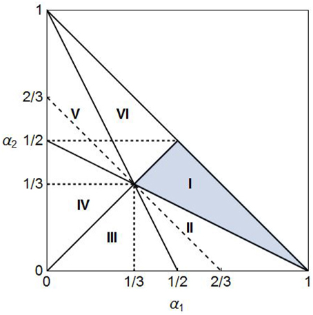
Figure 1. Divisions of the (α₁, α₂) plane with α₃ ≥ 0.

Region I is colored in gray and we will limit our analysis to it below. The line of α₂ = (2 − 3m)/2(1 − m) − α₁ is shown to be dotted and downward sloping¹. It is also checked that β₁ = 0, β₂ = 0, and β₃ = 0 hold, respectively, on the loci of α₂ = α₁, α₃ = α₂, and α₃ = 0. On these boundaries the three-delay Equation (2) is reduced to one of three two-delay equations, depending on which β_i value becomes zero. Matsumoto and Szidarovszky [11] consider a two delay equation that corresponds to the one with β₃ = 0. Their analytical method can be applied to the other two equations as well. In this study, we will confine our attention to the regions in which β_i > 0. Although, the parametric region I is a smaller part of the whole feasible region, the three delay model restricted to region I has more freedom concening the parametric choice than the two delay model that is defined only on the line α₂ = 1 − α₁.

2.1. Construction of Stability Switching Curves

Substituting an exponential solution $p_{\delta }(t)=e^{\lambda t}u$ into the linearized Equation (2) yields the corresponding characteristic equation

$\lambda -\alpha -{\beta }_1{e}^{-\lambda {\tau }_1}-{\beta }_2{e}^{-\lambda {\tau }_2}+{\beta }_3{e}^{-\lambda {\tau }_3}=0\left(3\right)$

Dividing the left hand side of Equation (3) by λ − α and denote the result by a(λ),

$a(\lambda )=1+a_1(\lambda )e^{-\lambda {\tau }_1}+a_2(\lambda )e^{-\lambda {\tau }_2}+a_3(\lambda )e^{-\lambda {\tau }_3}=0\left(4\right)$

with

$a_1(\lambda )=\frac{-{\beta }_1}{\lambda -\alpha }\text{, }{a}_2(\lambda )=\frac{-{\beta }_2}{\lambda -\alpha },a_3(\lambda )=\frac{{\beta }_3}{\lambda -\alpha }.$

Since λ = 0 is not a solution of Equation (3), a pair of pure imaginary roots must exist if stability switch occurs. We thus assume λ = iω, ω > 0 is a solution of Equation (3). For λ = iω,

$a_1(i\omega )=\frac{\alpha {\beta }_1+i{\beta }_1\omega }{{\alpha }^2+{\omega }^2}\text{ and }\left|a_1(i\omega )\right|=\frac{\left|{\beta }_1\right|}{\sqrt{{\alpha }^2+{\omega }^2}},$

$a_2(i\omega )=\frac{\alpha {\beta }_2+i{\beta }_2\omega }{{\alpha }^2+{\omega }^2}\text{ and }\left|a_2(i\omega )\right|=\frac{\left|{\beta }_2\right|}{\sqrt{{\alpha }^2+{\omega }^2}}$

and

$a_3(i\omega )=-\frac{\alpha {\beta }_3+i{\beta }_3\omega }{{\alpha }^2+{\omega }^2}\text{ and }\left|a_1(i\omega )\right|=\frac{{\beta }_3}{\sqrt{{\alpha }^2+{\omega }^2}}.$

Each term of a(iω) may be viewed as a vector in the complex plane. Hence solving a(iω) = 0 analytically is equivalent to constructing a quadrangle geometrically as shown in Figure 2 in which these four vectors are arranged from head to tail.

FIGURE 2

Figure 2. |1| and |a_j(iω)| for j = 1, 2, 3 form a quadrangle.

The determination of the stability switching surface in the (τ₁, τ₂, τ₃) plane is challenging². In order to make the problem manageable, we reduce the three-delay equation to a two-delay equation by fixing the value of τ₃ at a certain positive level and then construct the stability switching curve in the (τ₁, τ₂) plane in which we can apply the method used earlier in Matsumoto and Szidarovszky [11], and Gu et al. [14]. Notice that vector 1 is connected to vector $a_3(i\omega )e^{-i\omega {\tau }_3}$ in Figure 2. If the sum of these vectors is denoted by a_d(iω, τ₃),

$a_d(i\omega ,{\tau }_3)=1+a_3(i\omega )e^{-i\omega {\tau }_3},$

then a(λ) with λ = iω can be rewritten as

$a(i\omega )=a_d(i\omega ,{\tau }_3)+a_1(i\omega )e^{-i\omega {\tau }_1}+a_2(i\omega )e^{-i\omega {\tau }_2}.$

As already shown in Figure 2, a(iω) = 0 means that these three vectors in a(iω) must form a triangle having the dotted base with interior angles, θ₁ and θ₂. Sufficient and necessary conditions for forming a triangle are given by

$\begin{array}{l}(i)f_d(\omega )=\left|a_1(i\omega )\right|+\left|a_2(i\omega )\right|-\left|a_d(i\omega ,{\tau }_3)\right|\ge 0,\\ (ii)f_1(\omega )=\left|a_2(i\omega )\right|+\left|a_d(i\omega ,{\tau }_3)\right|-\left|a_1(i\omega )\right|\ge 0,\\ (iii)f_2(\omega )=\left|a_d(i\omega ,{\tau }_3)\right|+\left|a_1(i\omega )\right|-\left|a_2(i\omega )\right|\ge 0.& \left(5\right)\end{array}$

Each inequality condition implies that the length of any segment of the triangle is not greater than the sum of the lengths of the remaining two segments. Define the crossing frequency set Ω of all ω > 0 such that a(iω) = 0 holds for at least one delay combination (τ₁, τ₂, τ₃) ≥ 0. For ω = 0 in a(iω) leads to

${a(i\omega )|}_{\omega =0}=\frac{1}{\alpha }\left(\alpha +{\beta }_1+{\beta }_2-{\beta }_3\right)<0.$

This inequality implies 0 ∉ Ω.

By the law of cosine, we can determine the values of θ₁ and θ₂ of the triangle in Figure 2,

${\theta }_1(\omega )={\cos }^{-1}\left[\frac{{\left|a_d(i\omega ,{\tau }_3)\right|}^2+{\left|a_1(i\omega )\right|}^2-{\left|a_2(i\omega )\right|}^2}{2\left|a_d(i\omega ,{\tau }_3)\right|\left|a_1(i\omega )\right|}\right]$

and

${\theta }_2(\omega )={\cos }^{-1}\left[\frac{{\left|a_d(i\omega ,{\tau }_3)\right|}^2+{\left|a_2(i\omega )\right|}^2-{\left|a_1(i\omega )\right|}^2}{2\left|a_d(i\omega ,{\tau }_3)\right|\left|a_2(i\omega )\right|}\right].$

Vertices A and B maybe located above or below the horizontal axis and the slope of segment AB can be positive or negative. So we have eight possibilities to construct a quadrangle. However, a simple geometric consideration shows that there are only two different possibilities:

$\arg \left(a_1(i\omega )e^{-i\omega {\tau }_1}\right)+(2k-1)\pi -\arg (a_d(i\omega ,{\tau }_1))\pm {\theta }_1(\omega )=0$

and

$\arg \left(a_2(i\omega )e^{-i\omega {\tau }_2}\right)+(2n-1)\pi -\arg (a_d(i\omega ,{\tau }_1))\mp {\theta }_2(\omega )=0.$

Solving these equations for τ₁ and τ₂ yields the threshold values of the delays,

$\begin{array}{l}{\tau }_1^{\pm }(\omega ,k)=\frac{1}{\omega }[\arg (a_1(i\omega ))-\arg (a_d(i\omega ,{\tau }_3))+(2k-1)\pi \\ \pm {\theta }_1(\omega )]& \left(6\right)\end{array}$

and

$\begin{array}{l}{\tau }_2^{\mp }(\omega ,n)=\frac{1}{\omega }[\arg (a_2(i\omega ))-\arg (a_d(i\omega ,{\tau }_3))+(2n-1)\pi \\ \mp {\theta }_2(\omega )].& \left(7\right)\end{array}$

The stability switching curves consist of two sets of parametric segments,

$L_1(k,n)=\{{\tau }_1^{+}(\omega ,k),{\tau }_2^{-}(\omega ,n)\}\text{ for }k,n=0,1,2,...\left(8\right)$

and

$L_2(k,n)=\{{\tau }_1^{-}(\omega ,k),{\tau }_2^{+}(\omega ,n)\}\text{ for }k,n=0,1,2,...\left(9\right)$

where the parameter ω runs through the crossing frequency set Ω.

Substituting τ₁ = τ₂ = τ₃ = 0 into Equation (3) presents

$\lambda =\alpha +{\beta }_1+{\beta }_2-{\beta }_3=-fm<0.$

This inequality implies that the steady state with no delays is stable. Next, assuming that τ₁ = τ₂ = 0, we examine the existence of a threshold value of τ₃ at which the system loses stability. Without loss of generality, assuming λ = iω, ω > 0 and then substituting it into Equation (3) with τ₁ = τ₂ = 0 reduce the characteristic equation to

$i\omega -(\alpha +{\beta }_1+{\beta }_2)+{\beta }_3{e}^{-i\omega {\tau }_3}=0.$

We denote α + β₁ + β₂ by Δ where

$\Delta =f(1-m)\left(1-{\alpha }_1-{\alpha }_2-\frac{m}{1-m}\right)$

and break down the characteristic equation into the real and imaginary parts,

$\begin{array}{l}-\Delta +{\beta }_3\cos \omega {\tau }_3=0\\ \omega -{\beta }_3\sin \omega {\tau }_3=0.& \left(10\right)\end{array}$

Moving Δ and ω to the right hand side and adding the squared equations give

${\omega }^2={\beta }_3^2-{\Delta }^2$

where

${\beta }_3-\Delta =fm>0$

and

${\beta }_3+\Delta =2f(1-m)\left(\phi ({\alpha }_1)-{\alpha }_2\right)$

with

$\phi ({\alpha }_1)=\frac{2-3m}{2(1-m)}-{\alpha }_1.$

Notice that the dotted curve in Figure 1 is described by α₂ = φ(α₁). It is clear first that

${\beta }_3+\Delta ⋛0\text{ according to }\phi ({\alpha }_1)⋛{\alpha }_2$

and second that

${\beta }_3+\Delta <0\text{ if }m\ge 2/3.$

This leads to the following result.

Proposition 1. Given τ₁ = τ₂ = 0, the solution of delay system (1) is stable for any τ₃ ≥ 0 if the fundamentalists dominate over the chartists in the sense that m ≥ 2/3.

If β₃ + Δ > 0, then there is a ω such as $\stackrel{-}{\omega }=\sqrt{{\beta }_3^2-{\Delta }^2}>0.$ In this case, loss of stability for $\lambda =i\stackrel{-}{\omega }$ can be shown in the following way. The characteristic equation with τ₁ = τ₂ = 0 can be written as

${\beta }_3{e}^{-\lambda {\tau }_3}={\beta }_1+{\beta }_2+\alpha -\lambda .\left(11\right)$

Taking λ as a function of τ₃ and differentiating it with respect to τ₃ yield

$\begin{array}{l}\frac{d\lambda }{d{\tau }_3}=\frac{\lambda {\beta }_3{e}^{-\lambda {\tau }_3}}{1-{\tau }_3{\beta }_3{e}^{-\lambda {\tau }_3}}\\ =\frac{\lambda ({\beta }_1+{\beta }_2+\alpha -\lambda )}{1-{\tau }_3({\beta }_1+{\beta }_2+\alpha -\lambda )}\end{array}$

where the right hand side of Equation (11) are used. Substituting λ = iω and taking the real part of the resulting expression give

${\frac{d\left[\text{Re}\lambda \right]}{d{\tau }_3}|}_{\lambda =i\omega }=\text{Re}\left[\frac{\lambda ({\beta }_1+{\beta }_2+\alpha -\lambda )}{1-{\tau }_3({\beta }_1+{\beta }_2+\alpha -\lambda )}\right]=\text{Re}\left[\frac{{\omega }^2+i\omega ({\beta }_1+{\beta }_2)}{1-{\tau }_3({\beta }_1+{\beta }_2+\alpha )-i\omega }\frac{1+{\tau }_3({\beta }_1+{\beta }_2+\alpha )-i\omega }{1+{\tau }_3({\beta }_1+{\beta }_2+\alpha )-i\omega }\right]=\frac{{\omega }^2}{{\left[1-{\tau }_3({\beta }_1+{\beta }_2+\alpha )\right]}^2+{\omega }^2}>0.$

This inequality implies that all roots cross the imaginary axis at iω from left to right as τ₃ increases so stability is lost. Correspondingly, solving the first equation of Equation (10) for τ₃ presents the threshold value

${\overline{\tau }}_3({\alpha }_1,{\alpha }_2,m)=\frac{1}{\overline{\omega }}{\cos }^{-1}\left(\frac{\Delta }{{\beta }_3}\right)>0\left(12\right)$

and the system is stable for ${\tau }_3<{\stackrel{-}{\tau }}_3$ and unstable otherwise³. We summarize the results obtained so far.

Proposition 2. Given τ₁ = τ₂ = 0, the solution of delay system (1) is stable for ${\tau }_3<{\stackrel{-}{\tau }}_3({\alpha }_1,{\alpha }_2,m),$ loses stability for ${\tau }_3={\stackrel{-}{\tau }}_3({\alpha }_1,{\alpha }_2,m)$ and becomes unstable for all ${\tau }_3>{\stackrel{-}{\tau }}_3({\alpha }_1,{\alpha }_2,m)$ if the following condition holds,

${\alpha }_2<\phi ({\alpha }_1)$

whereas it is always stable for any τ₃ > 0 otherwise.

It is to be noticed that with τ₁ = τ₂ = 0, the three delay model is reduced to a one delay model and thus this stability result is essentially the same as the one of Qu and Wei [10]. In the next section we will proceed to the case of τ_i > 0 for i = 1, 2, 3.

3. Dynamics

Central to this study is the problem of dynamics associated with three fixed delays. This problem is complex and it seems unlikely that an analytical approach to nonlinear delay differential Equation (1) would generate fruitful results on dynamics as it might be difficult to solve the equation. In order to understand global dynamics with delays better, it is useful to take a numerical approach. To this end, we make several simplifying assumptions and then numerically examine dynamics of the asset price.

Assumption 1. f = 5, m = 0.4 and τ₃ = 5.

Assumption 2. α_i for i = 1, 2, 3 satisfy α₁ > α₂ > α₃ > 0.

Assumption 3. τ_i for i = 1, 2, 3 satisfy τ₁ < τ₂ < τ₃.

Since the parameter values in Assumption 1 are determined only for computational convenience, the main results to be obtained below hold for any other values, provided that m < 2/3. Assumption 2 implies that the more recent trend has the more weight. This is not necessary but simplifies the analysis. Under m = 0.4 of Assumption 1, region I is located above the line α₂ = φ(α₁) which is the dotted downward-sloping line passing through point (1/3, 1/3) in Figure 1. Due to Proposition 2, the stationary point is always stable in region I where α₂ > φ(α₁) if τ₁ = τ₂ = 0. Thus it is easy to see how increasing values of these delays affect stability of the steady state. Assumption 3 imposes a natural ordering among the three delays, that is, an older price has a longer delay.

The rest of this section is divided into three subsections. We will look at the τ₁-effect on dynamics caused by a change in τ₁ in Section Delay Effect I: τ₁-effect, explore the τ₂-effect in Section Delay Effect II: τ₂-effect, and focus on considerations of the τ₃-effect in Section Delay Effect III: τ₃-effect.

3.1. Delay Effect I: τ₁-effect

We start with the τ₁-effect and present some numerical examples to see how different values of τ₁ affect dynamics of Equation (1). We first check the triangle conditions. Subtracting the third equation from the second equation Equation in (5) yields

$f_1(\omega )-f_2(\omega )=\frac{6f(1-m)}{\sqrt{{\alpha }^2+{\omega }^2}}\left({\alpha }_2-\frac{1}{3}\right)\left(13\right)$

implying that the relative location of the curves of f₁(ω) and f₂(ω) depends on whether the value of α₂ is larger or less than 1/3. To simplify the analysis, we assume that the value of α₂ is kept constant at 1/3;

Assumption 4. α₂ = 1/3

Assumption 2 implies η_i > 0 for all i, that is, the weights of the delay prices to calculate the moving average are positive. Their relative magnitudes depend on the selected values of α_i and thus there are many possibilities. Among them, we will limit analysis to only two cases, η₁ = η₂ > η₃ if α₁ < 1/2 and η₃ > η₁ = η₂ if α₁ < 1/2 since Assumption 4 makes η₁ = η₂ always⁴. With Assumption 4, f₁(ω) = f₂(ω) holds regardless of the value of α₁. Further, f_i(ω) > 0, i = 1, 2, for ω > 0 which will be numerically confirmed below. Consequently, it is enough to verify only the location and the shapes of the f_d(ω) curve. We consider dynamics over an interval $\left[{\alpha }_1^0,2/3\right]$ of α₁. The left hand side extreme value, ${\alpha }_1^0\simeq 0.356$ is numerically determined so as to make the maximum of f_d(ω) equal to zero. Thus for ${\alpha }_1<{\alpha }_1^0$, f_d(ω) < 0 for all ω > 0, implying that one of the triangle conditions is always violated. The other extreme value, α₁ = 2/3, together with α₂ = 1/3 makes α₃ = 0 via α₂ = 1 − α₁. For α₁ > 2/3, the nonnegative condition α₃ ≥ 0 is violated. In the following numerical analysis, α₁ is increased from 6/15 to 9/15 with an increment of 1/15. The resultant four f_d(ω) curves are colored in black in Figure 3 where the red curve with α₁ = 1/2 and the blue curves with those extreme values are also depicted. The corresponding f₁(ω) = f₂(ω) curves are illustrated in the dotted curves with the same color and are seen to be positive for all ω ≥ 0. In the gray region below the lower blue curve, no stability switch occurs and thus the steady state is stable. We do not consider the τ₁-effect there. On the other hand, the gray region above the upper blue curve is not feasible and thus eliminated from consideration. Figure 3 also illustrates various shapes of the f_d(ω) curves and shows that increasing α₁ shifts the curve upward and removes its unevenness. Indeed, the lower blue curve with ${\alpha }_1={\alpha }_1^0$ located at the bottom of the yellow region is high-wave shaped while the higher blue curve with α₁ = 2/3 at the top is monotonically downward-sloping. In addition, as the red curve passes through the origin, we then see that the curves below the red curve have two intersections with the horizontal axis and the curves above have only one intersection.

FIGURE 3

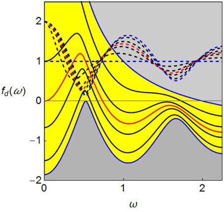
Figure 3. The f_d(ω) curves with various values of α₁.

To be more specific, we pick up α₁ = 6/15 and construct a stability switching curve. The corresponding f_d(ω) curve is the black one just above the lower blue curve in Figure 3 and intersects the horizontal axis twice at

${\overline{\omega }}_1\simeq 0.438\text{ and }{\overline{\omega }}_2\simeq \mathrm{0.582.}$

The triangle conditions in Equation (5) hold for $\omega \in \Omega =\left[{\stackrel{-}{\omega }}_1,{\stackrel{-}{\omega }}_2\right].$ We now ready to derive the stability switching curves, L₁(k, n) and L₂(k, n) defined in (8) and (9). Taking k = n = 1, we obtain the points of ${\tau }_1^{\pm }(\omega ,1)$ and ${\tau }_2^{\mp }(\omega ,1)$ by changing values of ω with increment 0.0002 inside the interval $\left[{\stackrel{-}{\omega }}_1,{\stackrel{-}{\omega }}_2\right]$ and then plot these points in the (τ₁, τ₂) plane. In Figure 4A, segment L₂(1, 1) is illustrated as a real curve in the region above the diagonal and segment L₁(1, 1) is a dotted curve in the region below⁵. Two segments form an elliptical-shaped closed curve having the starting point $S=({\tau }_1^{+}({\stackrel{-}{\omega }}_1,1),{\tau }_2^{-}({\stackrel{-}{\omega }}_1,1))$ and the ending point $E=({\tau }_1^{-}({\stackrel{-}{\omega }}_2,1),{\tau }_2^{+}({\stackrel{-}{\omega }}_2,1))$ on the diagonal where, for i = 1, 2,

${\tau }_i^{\pm }({\overline{\omega }}_1,1)={\tau }^s\simeq 8.478\text{ and }{\tau }_i^{\pm }({\overline{\omega }}_2,1)={\tau }^e\simeq \mathrm{2.789.}$

FIGURE 4

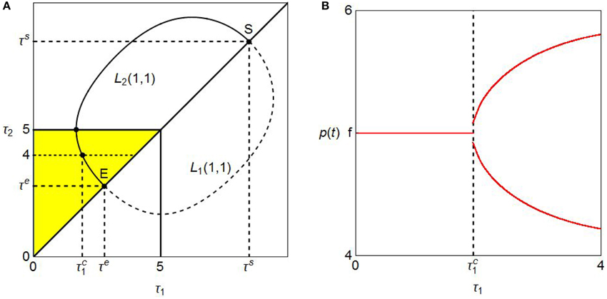
Figure 4. Dynamics for α₁ = 6/15 and α₂ = 1/3: (A) Stability region, (B) Bifurcation diagram.

Since the delays have two constraints, τ_i ≤ 5 for i = 1, 2 and τ₁ < τ₂ due to Assumptions 1 and 3, the feasible region should be above the diagonal line and subject to τ₂ ≤ 5. It is colored in yellow and further sub-divided into two sub-regions by the L₂(1, 1) segment that intersects two lines, one is the diagonal at (τ^e, τ^e) and the other is the horizontal line at τ₂ = 5⁶.

It is clear from the yellow region that stability is preserved for τ₁ and τ₂ such as $0<{\tau }_1<{\tau }^e$ and ${\tau }_1<{\tau }_2<{\tau }^e$. When the varying pair (τ₁, τ₂) with ${\tau }_2>{\tau }^e$crosses the L₂(1, 1) segment, we have the stability switching as the real part of at least one eigenvalue turns to be positive and then the stationary point loses stability. To see this, we perform a simulation by increasing the value of τ₁ along the dotted horizontal line at τ₂ = 4 that crosses the L₂(1, 1) curve at point (${\tau }_1^c,4$) with ${\tau }_1^c\simeq 1.640$⁷. The numerical results are summarized in Figure 4B in which a bifurcation diagram with respect to τ₁ is depicted. For ${\tau }_1\le {\tau }_1^c$, a pair of (τ₁, 4) stays within the stability region. So the stationary point p* = f is stable and the corresponding part of the bifurcation diagram is a horizontal line at p(t) = f. Once ${\tau }_1>{\tau }_1^c,$ the pair is in the instability region above the L₂(1, 1) segment. The stationary point, therefore, loses stability and bifurcates to a limit cycle having two extreme values (i.e., maximum and minimum). The existence of the limit cycle is confirmed by the Hopf bifurcation theorem. Figure 4B further implies that the limit cycle becomes larger as τ₁ gets larger and the stability is never regained for τ₁ ≤ 4⁸. The τ₁-effect is summarized as follows:

Proposition 3. Stability of dynamic Equation (1) with respect to τ₁ depends on the selected value ${\stackrel{-}{\tau }}_2$ of τ₂;

$\begin{array}{l}\begin{array}{cc}If {\overline{\tau }}_2\le {\tau }^e,& then the steady state is stable for {\tau }_1<{\overline{\tau }}_2;\end{array}\\ \begin{array}{ll}If{\overline{\tau }}_2>{\tau }^e,\hfill & then there is the threshold value {\tau }_1^c such that the\hfill \\ \hfill & steady state is stable for {\tau }_1<{\tau }_1^c and loses stability for\hfill \\ \hfill & {\tau }_1\ge {\tau }_1^c.\hfill \end{array}\end{array}$

where ${\tau }_1^c$ is the τ₁-point of the intersection of the switching curve and the horizontal line at ${\stackrel{-}{\tau }}_2$.

Taking various values of α₁ from the interval $\left[{\alpha }_1^0,2/3\right]$ and constructing the stability switching curves, we detect the τ₁-effect more. In Figure 5A, the switching curves with various values of α₁ are illustrated and their end-points on the diagonal are denoted by the green dots. The upper most blue curve has ${\alpha }_1={\alpha }_1^0$ and the lower most blue curve has α₁ = 2/3 while the curve shifts downward as α₁ increases from ${\alpha }_1^0$ to 2/3. As far as the curve is single-valued in τ₂, we have essentially the same result on the τ₁-effect as in the case of τ₁ = 6/15: fixing the value of τ₂ at some level and increasing the value of τ₁, the stability is preserved for τ₁ below the threshold value ${\tau }_1^c$ and it is lost for ${\tau }_1>{\tau }_1^c.$ As seen in Figure 5A, this threshold value becomes smaller as the value of α₁ becomes larger⁹, a larger value of α₁ reinforces the destabilizing τ₁-effect.

FIGURE 5

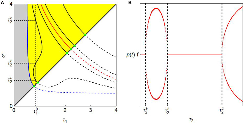
Figure 5. Delay destabilizing and stabilizing effects: (A) Stability switching curves; (B) Bifurcation diagram.

3.2. Delay Effect II: τ₂-effect

Taking τ₁ fixed, we are next concerned with the τ₂-effect, how changes in the value of τ₂ affect dynamics. We first return to Figure 4A in which both values of α₁ and α₂ are fixed at 6/15 and 1/3, respectively. The downward-sloping shape of the switching curve in the yellow region indicates that changing the value of τ₂ with constant τ₁ may generate similar effect to the τ₁-effect. Let ${\tau }_1^m$ denote the τ₁-value of the intersection of the stability switching curve and the horizontal line at τ₂ = 5¹⁰. If τ₁ is selected to be less than ${\tau }_1^m,$ then the steady state is stable for any τ₂ that should be above the diagonal and ≤5. If ${\tau }_1^m<{\tau }_1<{\tau }^e,$ then the steady state is stable for ${\tau }_2<{\tau }_2^c$ and bifurcates to a limit cycle for ${\tau }_2>{\tau }_2^c$ where ${\tau }_2^c$is defined in the same way as ${\tau }_1^c$ and depends on the selected value of τ₁. One more case exists and is specific to the τ₂-effect, namely, if ${\tau }_1>{\tau }^e,$ any feasible pair of τ₁ and τ₂ is in the unstable region so the steady state is unstable.

We now turn attention again to Figure 5A and consider the τ₂-effect when α₁ is increased but α₂ is still fixed at 1/3. It is already seen that the stationary point is stable in the region left to the stability switching curve and increasing the value of α₁ shifts the switching curve leftward. The stability switching curve with α = α₀ is not depicted as it is located outside Figure 5A. The shift of the curve implies that a larger value of α₁ reinforces the destabilizing τ₂-effect in the sense that it makes the stability region smaller. In addition, we have interesting dynamic phenomenon when the switching curve with α₁ being close to 2/3 has forward- and backward-bending segments. This shape suggests the stability loss and gain with respect to τ₂. If the initial point of (τ₁, τ₂) is selected on the diagonal such that the stationary point is stable, then the vertical line standing at this value of τ₁ denoted as ${\tau }_1^0=0.85$ crosses the stability switching curve three times at

${\tau }_2^a\simeq 1.014,{\tau }_2^b\simeq 1.687\text{ and }{\tau }_2^c\simeq 3.359$

as illustrated in Figure 5A. That is, the stability is lost at the first intersection and a limit cycle emerges. The cycle is getting larger and then smaller to merge the steady state at the value of the second intersection at which the stability is regained. Further increasing τ₂ crosses the stability switching curve again at which the stability is lost again. The corresponding bifurcation diagram is given in Figure 5B in which the stability losses and gains are shown. This τ₂-effect is summarized as follows:

Proposition 4. With a value of τ₁ being close to 2/3, the increasing delay τ₂ has a double edge effect in a sense that it can destabilize the market price to generate a limit cycle, then stabilize it and later destabilize it again.

3.3. Delay Effect III: τ₃-effect

We now look into the τ₃-effect, the effect caused by changing the value of τ₃. To this end, α₁ = (6 − 0.1)/12 is taken and dynamics with three different values of τ₃, τ₃ = 5, τ₃ = 6, and τ₃ = 7, are considered. The corresponding switching curves are illustrated in different colors in Figure 6A (that is, a blue curve with τ₃ = 5, red curves with τ₃ = 6, and black curves with τ₃ = 7). As τ₃ increases, it is observed first that the feasible regions of τ₁ and τ₂ increase since the upper bound of τ₂ becomes larger and second that the downward-sloping switching curve shifts upward, which implies an enlargement of the stability region. It is further observed that island-shaped switching curves emerge for τ₃ = 6 and τ₃ = 7 and the steady state is unstable inside them. To detect the reason why the island-shaped region is born under larger values of τ₃, we draw the green f₁(ω) = f₂(ω) curve and the red f_d(ω) curve for τ₃ = 7 in Figure 6B. It is seen that f₁(ω) = f₂(ω) > 0 for ω > 0 and the larger τ₃ value makes the second hump of the f_d(ω) curve high enough to cross over the horizontal line. As a result, the red curve intersects the horizontal line four times at

${\omega }_1\simeq 0.104,{\omega }_2\simeq 0.562,{\omega }_3\simeq 1.059\text{and}{\omega }_{\text{4}}\simeq \text{1}.\text{256}.$

FIGURE 6

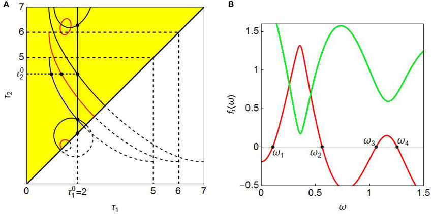
Figure 6. τ₃-effects on switching curves: (A) Stability switching curves; (B) Triangle conditions.

In consequence, the triangle conditions (5) hold in the two intervals, [ω₁, ω₂] and [ω₃, ω₄]. It is verified that the switching curve defined on [ω₁, ω₂] is downward-sloping and the one on [ω₃, ω₄] forms an island shape. Both curves are colored in black. The existence of the smaller red islands indicates that the f_d(ω) curve also intersects the horizontal axis four times even when τ₃ = 6. A critical value of τ₃ for the birth of the island is somewhere between τ₃ = 5 and τ₃ = 6, for which the maximum of the second hump of f_d(ω) becomes zero.

Proposition 5. As far as τ₃ is relatively small, increasing the value of τ₃ stabilizes the steady state by shifting the downward-sloping switching curve upward whereas for a relatively larger value, increasing value of τ₃ additionally generates an island-shaped switching curve within which the steady state is unstable.

To see the τ₃-effect on dynamics, we perform two simulations. In the first simulation, we increase the value of τ₁ along the horizontal line at ${\tau }_2={\tau }_2^0(\simeq 4.356)$. This line successively crosses the stability switching curves, the blue curve at ${\tau }_1^a(\simeq 0.972),$ the red curve at ${\tau }_1^b(\simeq 1.372)$ and the black curve at ${\tau }_1^c(=2)$. Although, these bifurcating values are denoted as black dots, they are not labeled in Figure 6A to avoid confusion. The corresponding bifurcation diagrams are illustrated in Figure 7A in which the black curve is depicted first, the red curve is then put on it and finally the blue curve is further placed upon. Each diagram has a qualitatively similar shape as the one shown in Figure 4B, that is, the steady state loses stability at the bifurcation value and a limit cycle emerges for a larger value of τ₁. Thus larger τ₃ value does not alter qualitative aspects of the τ₁-effect, however, does affect its quantitative aspects because the bifurcation value of τ₁ becomes larger as τ₃ increases. Increasing value of τ₃ enhances the stabilizing τ₁-effect by delaying the loss of stability.

FIGURE 7

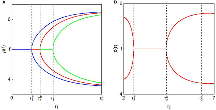
Figure 7. Delay effects on dynamics: (A) τ₁-effect; (B) τ₂-effect.

In the second simulation, we shift the emphasis away from the τ₁-effect to the τ₂-effect. Fixing τ₃ = 7 and starting at point (2, 2) on the diagonal, we increase the value of τ₂ from 2 to 7 along the vertical real line at ${\tau }_1={\tau }_1^0(=2)$ in Figure 6A. The line crosses the lower black island-shaped curve at ${\tau }_2^a(\simeq 2.563)$, the black downward sloping curve at ${\tau }_2^b(\simeq 4.356)$ and then upper black circle-shaped curve at ${\tau }_2^c(\simeq 6.283)$. These threshold values are not labelled in Figure 6A by the same reason as before. The simulation results are given in Figure 7B in which stability gain and loss occur in the following way:

(i) we initially have a unstable steady state (in other words, a stable limit cycle) when the initial point is selected on the diagonal in Figure 6A¹¹, that is inside the half black circle. The real part of one eigenvalue is positive.

(ii) the limit cycle becomes smaller as τ₂ increases from 2 to ${\tau }_2^a$ and merges with the steady state for ${\tau }_2={\tau }_2^a$ at which instability is switched to stability. The positive real part turns to be negative when the delay τ₂ crosses the imaginary axis from left to right.

(iii) for ${\tau }_2^a<{\tau }_2<{\tau }_2^b,$ the model has a stable steady state and stability loss occurs for ${\tau }_2={\tau }_2^b$. The real parts of at least one eigenvalue turn to be positive again when the delay τ₂ crosses the imaginary axis.

(iv) for ${\tau }_2>{\tau }_2^b,$ Figure 7B suggests the existence of stable limit cycles and the instability of the steady state. Although further increasing τ₂ intersects the island switching curve at point $(2,{\tau }_2^c)$ at which the real part of another eigenvalue changes sign. However no stability switch occurs, since there is already at least one other eigenvalue with positive real part.

Proposition 6. Increasing the value of τ₃ does not affect essentially dynamics with respect to τ₁ and can affect the dynamics with respect to τ₂ as it can generate multiple stability switching.

4. Concluding Remarks

This paper constructs a heterogeneous agent model with three fixed delays and considers its dynamic behavior both analytically and numerically. The dependence of the delay effects on the changes in the lengths of the delays is also studied. The common result is that a longer delay can destabilize the market and can give rise to cyclic oscillations around the equilibrium (i.e., fundamental) price. This result clarifies the instability condition and thus complements the numerical study of Dibeh [9]. In addition, it is found that under multiple delays, stability loss and gain repeatedly occur as the length of a delay increases. He and Zheng [6] observed this phenomenon in a financial market model with continuously distributed time delay with finite memory length that involved infinitely many past price observations and called it the double edge effect. Our model is based on one, two or three past observations. It is thus shown in this paper that the same effect can occur even under finite delay information. In our future research the model of this paper will be extended to involve two risky assets and the stability and instability of the equilibrium will be examined in the extended models.

Author Contributions

AM: Performs simulations; FS: Constructs the model.

Conflict of Interest Statement

The authors declare that the research was conducted in the absence of any commercial or financial relationships that could be construed as a potential conflict of interest.

Acknowledgments

The authors thank two referees for very helpful comments and highly appreciate the finanical supports from the MEXT-Supported Program for the Strategic Research Foundation at Private Universities 2013-2017, the Japan Society for the Promotion of Science (Grant-in-Aid for Scientific Research (C), 25380238, 26380316 and 16k03556) and Chuo University (Joint Research Grant). The usual disclaimers apply.

Footnotes

1. ^m = 0.4 is assumed and we will refer to this line later.

2. ^It is possible to have a switching surface in the 3D space. See Almodaresi and Bozorg [12] and Gu and Naghnaeian [13].

3. ^Solving the second equation of Equation (10) for τ₃ gives the same result in a different form.

4. ^The remaining cases will be examined in a subsequent paper.

5. ^The segment L_i(k, n) shifts upward if n increases and rightward if k increases. For (k, n)/2 and (k, n) = 0, the switching segments are defined but located ouside of the region with τ_i ≤ 5 for i = 1, 2, so they are not depicted in Figure 4A.

6. ^The τ₁-value of the intersection is obtained in the following way: first solving ${\tau }_2^{+}(\omega ,1)=5$ for ω yields a solution ω_m ≃ 0.560 and then substituting it into ${\tau }_1^{-}(\omega ,1)$ gives ${\tau }_1^m\simeq 0.887.$ So the black segment depicted in the yellow region is defined for ω ∈ [ω_m, ω₂].

7. ^It is possible to obtain this value by following the same procedure with which we obtained the value of ${\tau }_1^m$ just above.

8. ^Mathematically, it might be possible to regain stability for τ₁ > 4. However, economically it is not the case as τ₁ ≤ τ₂ ≤ 5 is imposed by Assumptions 1 and 3.

9. ^This is not the case of the non-monotonics curve with α₁ = 9/15.

10. ^“${\tau }_1^m$” is not labeled in Figure 4A to avoid figure congestion.

11. ^More precisely, we select a constant initial function, g(t) = 2 for t ≤ 0.

References

1. Hommes C. Heterogeneous agent models in economics and finance. In: Tesfatsion L, Judd KL, editors. Handbook of Computational Economics, Agent-based Computational Economics, II. North-Holland: Amsterdam (2006). p. 1109–86.

Google Scholar

2. Chiarella C, He XZ, Hommes C. A dynamic analysis of moving average rules. J Econ Dyn Control (2006) 30:1729–53. doi: 10.1016/j.jedc.2005.08.014

CrossRef Full Text | Google Scholar

3. Zeeman E. On the unstable behavior of stock exchanges. J Math Econ. (1974) 1:39–49.

Google Scholar

4. Beja A, Goldman M. On the dynamic behavior of prices in disequilibrium. J Finance (1980) 35:235–48. doi: 10.2307/2327380

CrossRef Full Text | Google Scholar

5. Chiarella C. The dynamics of speculative behavior. Ann Oper Res. (1992) 37:101–23.

Google Scholar

6. He XZ, Zheng M. Dynamics of moving average rules in a continuous-time financial market model. J Econ Behav Organ. (2010) 76:615–34. doi: 10.1016/j.jebo.2010.08.005

CrossRef Full Text | Google Scholar

7. He XZ, Li K. Heterogeneous beliefs and adaptive behavior in a continuous-time asset price model. J Econ Dyn Control (2012) 36:973–87. doi: 10.1016/j.jedc.2012.02.002

CrossRef Full Text | Google Scholar

8. Xu X, Liu J, Guo L, Xu Z. Oscillatory dynamics in a continuous-time delay asset price model with dynamical fundamental price. Comput Econ. (2015) 45:517–29. doi: 10.1007/s10614-014-9428-9

CrossRef Full Text | Google Scholar

9. Dibeh G. Speculative dynamics in a time-delay model of asset prices. Physica A (2005) 355:199–208. doi: 10.1016/j.physa.2005.02.084

CrossRef Full Text | Google Scholar

10. Qu Y, Wei J. Global hopf bifurcation analysis for a time-delayed model of asset prices. Discrete Dyn Nat Soc. (2010) 2010:432821. doi: 10.1155/2010/432821

CrossRef Full Text | Google Scholar

11. Matsumoto A, Szidarovszky F. Heterogeneous Agent Model of Asset Price with Time Delays. IERCU Discussion Paper #247, Institute of Economic Research, Chuo University (2015).

12. Almodaresi A, Bozorg M. Stability crossing surfaces for linear time-delay systems with three delays. Int J Control (2009). 82:2304–10. doi: 10.1080/00207170903037739

CrossRef Full Text | Google Scholar

13. Gu K. Naghnaeian M. On stability crossing set for systems with three delays. IEEE Trans Automat Contr. (2011) 56:11–26. doi: 10.1109/TAC.2010.2050162

CrossRef Full Text | Google Scholar

14. Gu K, Niculescu S, Chen J. On stability crossing curves for general systems with two delays. J Math Anal Appl. (2005) 311:231–53. doi: 10.1016/j.jmaa.2005.02.034

CrossRef Full Text | Google Scholar