A Fixed-Point of View on Gradient Methods for Big Data

1. Introduction

One of the main recent trends within machine learning and data analytics using massive data sets is to leverage the inferential strength of the vast amounts of data by using relatively simple, but fast, optimization methods as algorithmic primitives [1]. Many of these optimization methods are modifications of the basic gradient descent (GD) method. Indeed, computationally more heavy approaches, such as interior point methods, are often infeasible for a given limited computational budget [2].

Moreover, the rise of deep learning has brought a significant boost for the interest in gradient methods. Indeed, a major insight within the theory of deep learning is that for typical high-dimensional models, e.g., those represented by deep neural networks, most of the local minima of the cost function (e.g., the empirical loss or training error) are reasonably close (in terms of objective value) to the global optimum [3]. These local minima can be found efficiently by gradient methods such as stochastic gradient descent (SGD), which is considered the de-facto standard algorithmic primitive for training deep neural networks [3].

This paper elaborates on the interpretation of some basic gradient methods such as GD and its variants as fixed-point iterations. These fixed-point iterations are obtained for operators associated with the convex objective function. Emphasizing the connection to fixed-point theory unleashes some powerful tools, e.g., on the acceleration of fixed-point iterations [4] or inexact fixed-point iterations [5, 6], for the analysis and construction of convex optimization methods.

In particular, we detail how the convergence of the basic GD iterations can be understood from the contraction properties of a specific operator which is associated naturally with a differentiable objective function. Moreover, we work out in some detail how the basic GD method can be accelerated by modifying the operator underlying GD in a way that preserves its fixed-points but decreases the contraction factor which implies faster convergence by the contraction mapping theorem.

1.1. Outline

We discuss the basic problem of minimizing convex functions in Section (2). We then derive GD, which is a particular first order method, as a fixed-point iteration in Section (3). In Section (4), we introduce one of the most widely used computational models for convex optimization methods, i.e., the model of first order methods. In order to assess the efficiency of GD, which is a particular instance of a first order method, we present in Section (5) a lower bound on the number of iterations required by any first order method to reach a given sub-optimality. Using the insight provided from the fixed-point interpretation we show how to obtain an accelerated variant of GD in Section (6), which turns out to be optimal in terms of convergence rate.

1.2. Notation

The set of natural numbers is denoted ℕ := {1, 2, …}. Given a vector $\text{x}={(x_1,\dots ,x_n)}^T\in {ℂ}^n$, we denote its lth entry by x_l. The (hermitian) transpose and trace of a square matrix A ∈ ℂ^n×n are denoted (A^H) A^T and tr{A}, respectively. The Euclidian norm of a vector x is denoted $\Vert \text{x}\Vert :=\sqrt{{\text{x}}^H\text{x}}$. The spectral norm of a matrix M is denoted $||\text{M}||:=\underset{\Vert \text{x}\Vert =1}{max}||\text{M}\text{x}||$. The spectral decomposition of a positive semidefinite (psd) matrix Q ∈ ℂ^n×n is Q = UΛU^H with matrix U = (u⁽¹⁾, …, u⁽ⁿ⁾) whose columns are the orthonormal eigenvectors u⁽ⁱ⁾ ∈ ℂⁿ of Q and the diagonal matrix Λ containing the eigenvalues λ₁(Q) ≥ … ≥ λ_n(Q) ≥ 0. For a square matrix M, we denote its spectral radius as ρ(M) := max{|λ| : λ is an eigenvalue of M}.

2. Convex Functions

A function f(·):ℝⁿ → ℝ is convex if

$\begin{array}{l}f((1-\alpha )\text{x}+\alpha \text{y})\le (1-\alpha )f(\text{x})+\alpha f(\text{y})\end{array}$

holds for any x, y ∈ ℝⁿ and α ∈ [0, 1] [2]. For a differentiable function f(·) with gradient ∇f(x), a necessary and sufficient condition for convexity is [7, p. 70]

$\begin{array}{l}f(\text{y})\ge f(\text{x})+{(\text{y}-\text{x})}^T\nabla f(\text{x}),\end{array}$

which has to hold for any x, y ∈ ℝⁿ.

Our main object of interest in this paper is the optimization problem

$\begin{array}{ll}{\text{x}}_0\in {\displaystyle \underset{\text{ x}\in {ℝ}^n}{ arg min}}f(\text{x}).\hfill & (1)\end{array}$

Given a convex function f(x), we aim at finding a point x₀ with lowest function value f(x₀), i.e., $f(x_0)={\min }_{x}f(x)$.

In order to motivate our interest in optimization problems like Equation (1), consider a machine learning problem based on training data ${X}:={\left\{{\text{z}}^{(i)}\right\}}_{i=1}^N$ consisting of N data points z⁽ⁱ⁾ = (d⁽ⁱ⁾, y⁽ⁱ⁾) with feature vector d⁽ⁱ⁾ ∈ ℝⁿ (which might represent the RGB pixel values of a webcam snapshot) and output or label y⁽ⁱ⁾ ∈ ℝ (which might represent the local temperature during the snapshot). We wish to predict the label y⁽ⁱ⁾ by a linear combination of the features, i.e.,

$\begin{array}{ll}{y}^{(i)}\approx {\text{x}}^T{\text{d}}^{(i)}.& (2)\end{array}$

The choice for the weight vector x ∈ ℝⁿ is typically based on balancing the empirical risk incurred by the predictor (2), i.e.,

$\begin{array}{l}(1/N){\displaystyle \sum _{i=1}^N}{(y^{(i)}-{\text{x}}^T{\text{d}}^{(i)})}^2,\end{array}$

with some regularization term, e.g., measured by the squared norm ‖x‖². Thus, the learning problem amounts to solving the optimization problem

$\begin{array}{ll}{\text{x}}_0={\displaystyle \underset{\text{x}\in {ℝ}^n}{arg min}}(1/N){\displaystyle \sum _{i=1}^N}{(y^{(i)}-{\text{x}}^T{\text{d}}^{(i)})}^2+\lambda \Vert \text{x}{\Vert }^2.& (3)\end{array}$

The learning problem (3) is precisely of the form (1) with the convex objective function

$\begin{array}{ll}f(\text{x})≔(1/N){\displaystyle \sum _{i=1}^N}{(y^{(i)}-{\text{x}}^T{\text{d}}^{(i)})}^2+\lambda \Vert \text{x}{\Vert }^2.& (4)\end{array}$

By choosing a large value for the regularization parameter λ, we de-emphasize the relevance of the training error and thus avoid overfitting. However, choosing λ too large induces a bias if the true underlying weight vector has a large norm [3, 8]. A principled approach to find a suitable value of λ is cross validation [3, 8].

2.1. Differentiable Convex Functions

Any differentiable function f(·) is accompanied by its gradient operator

$\begin{array}{ll}\nabla f:{ℝ}^n\to {ℝ}^n,\text{x}\mapsto \nabla f(\text{x}).& (5)\end{array}$

While the gradient operator ∇f is defined for any (even non-convex) differentiable function, the gradient operator of a convex function satisfies a strong structural property, i.e., it is a monotone operator [9].

2.2. Smooth and Strongly Convex Functions

If all second order partial derivatives of the function f(·) exist and are continuous, then f(·) is convex if and only if [7, p.71]

$\begin{array}{l}{\nabla }^{2}f(\text{x})⪰\text{0}\mathrm{\text{ for every }}\text{x}\in {ℝ}^n.\end{array}$

We will focus on a particular class of twice differentiable convex functions, i.e., those with Hessian ∇²f(x) satisfying

$\begin{array}{ll}L\le {\lambda }_l({\nabla }^{2}f(\text{x}))\le U\mathrm{\text{ for every }}\text{x}\in {ℝ}^n,& (6)\end{array}$

with some known constants U ≥ L > 0.

The set of convex functions f(·):ℝⁿ → ℝ satisfying (6) will be denoted ${{S}}_n^{L,U}$. As it turns out, the difficulty of finding the minimum of some function $f(·)\in {{S}}_n^{L,U}$ using gradient methods is essentially governed by the

$\begin{array}{ll}\mathrm{\text{condition number }}\kappa ≔U/L\mathrm{\text{ of the function class }}{{S}}_n^{L,U}.& (7)\end{array}$

Thus, regarding the difficulty of optimizing the functions $f(·)\in {{S}}_n^{L,U}$, the absolute values of the bounds L and U in (6) are not crucial, only their ratio κ = U/L is.

One particular sub-class of functions $f(·)\in {{S}}_n^{L,U}$, which is of paramount importance for the analysis of gradient methods, are quadratic functions of the form

$\begin{array}{ll}f(\text{x})=(1/2){\text{x}}^T\text{Q}\text{x}+{\text{q}}^T\text{x}+c,& (8)\end{array}$

with some vector q ∈ ℝⁿ and a psd matrix Q ∈ ℝ^n×n having eigenvalues λ(Q) ∈ [L, U]. As can be verified easily, the gradient and Hessian of a quadratic function of the form (8) are obtained as ∇f(x) = Qx+q and ∇²f(x) = Q, respectively.

It turns out that most of the results (see below) on gradient methods for minimizing quadratic functions of the form (8), with some matrix Q having eigenvalues λ(Q) ∈ [L, U], apply (with minor modifications) also when expanding their scope from quadratic functions to the larger set ${{S}}_n^{L,U}$. This should not come as a surprise, since any function $f(·)\in {{S}}_n^{L,U}$ can be approximated locally around a point x₀ by a quadratic function which is obtained by a truncated Taylor series [10]. In particular, we have Rudin [10, Theorem 5.15]

$\begin{array}{l}f(\text{x})=f({\text{x}}_0)+{(\text{x}-{\text{x}}_0)}^T\nabla f({\text{x}}_0)\\ +(1/2){(\text{x}-{\text{x}}_0)}^T{\nabla }^{2}f(\text{u})(\text{x}-{\text{x}}_0),& (9)\end{array}$

where u = ηx + (1−η)x₀ with some η ∈ [0, 1].

The crucial difference between the quadratic function (8) and a general function $f(·)\in {{S}}_n^{L,U}$ is that the matrix ∇²f(z) appearing in the quadratic form in (9) typically varies with the point x. In particular, we can rewrite (9) as

$\begin{array}{l}f(\text{x})=\\ f({\text{x}}_0)+{(\text{x}-{\text{x}}_0)}^T\nabla f({\text{x}}_0)+(1/2){(\text{x}-{\text{x}}_0)}^T\text{Q}(\text{x}-{\text{x}}_0)\\ +(1/2){(\text{x}-{\text{x}}_0)}^T({\nabla }^{2}f(\text{z})-\text{Q})(\text{x}-{\text{x}}_0),& (10)\end{array}$

with $\text{Q}={\nabla }^{2}f({\text{x}}_0)$. The last summand in (10) quantifies the approximation error

$\begin{array}{l}\epsilon (\text{x})≔f(\text{x})-\tilde{f}(\text{x})\\ =(1/2){(\text{x}-{\text{x}}_0)}^T({\nabla }^{2}f(\text{z})-\text{Q})(\text{x}-{\text{x}}_0)& (11)\end{array}$

obtained when approximating a function $f(·)\in {{S}}_n^{L,U}$ with the quadratic $\tilde{f}(\text{x})$ obtained from (8) with the choices

$\begin{array}{l}\text{Q}={\nabla }^{2}f({\text{x}}_0),\\ \text{q}=\nabla f({\text{x}}_0)-\text{Q}{\text{x}}_0\mathrm{\text{ and}}\\ c=f({\text{x}}_0)+(1/2){\text{x}}_0^T\text{Q}{\text{x}}_0-{\text{x}}_0^T\nabla f({\text{x}}_0).\end{array}$

According to (6), which implies $ǁ{\nabla }^{2}f(x_0)ǁ,ǁ{\nabla }^{2}f(z)ǁ\le U$, we can bound the approximation error (11) as

$\begin{array}{l}\epsilon (\text{x})\le U\Vert \text{x}-{\text{x}}_0{\Vert }^2.\end{array}$

Thus, we can ensure a arbitrarily small approximation error ε by considering f(·) only over a neighborhood ${B}({\text{x}}_0,r):=\left\{\text{x}:\Vert \text{x}-{\text{x}}_0\Vert \le r\right\}$ with sufficiently small radius r > 0.

Let us now verify that learning a (regularized) linear regression model (cf. 3) amounts to minimizing a convex quadratic function of the form (8). Indeed, using some elementary linear algebraic manipulations, we can rewrite the objective function in (4) as a quadratic of the form (8) using the particular choices Q = Q_LR and q = q_LR with

$\begin{array}{ll}{\text{Q}}_{\text{LR}}≔\lambda \text{I}+\frac{1}{N}{\displaystyle \sum _{i=1}^N}{\text{d}}^{(i)}{(\text{d}}^{(i)}){}^T,\mathrm{\text{and }}{\text{q}}_{\text{LR}}≔\frac{2}{N}{\displaystyle \sum _{i=1}^N}{y}^{(i)}{\text{d}}^{(i)}.& (12)\end{array}$

The eigenvalues of the matrix Q_LR obey [11]

$\begin{array}{l}\lambda \le {\lambda }_l{(\text{Q}}_{\text{LR}})\le \lambda +{\lambda }_1({\text{D}}^T\text{D})\end{array}$

with the data matrix D := (d⁽¹⁾, …, d^(N)) ∈ ℝ^n×N. Hence, learning a regularized linear regression model via (3) amounts to minimizing a convex quadratic function $f(·)\in {{S}}_n^{L,U}$ with L = λ and $U=\lambda +{\lambda }_1({\text{D}}^T\text{D})$, where λ denotes the regularization parameter used in (3).

3. Gradient Descent

Let us now show how one of the most basic methods for solving the problem (1), i.e., the GD method, can be obtained naturally as fixed-point iterations involving the gradient operator ∇f (cf. 5).

Our point of departure is the necessary and sufficient condition [7]

$\begin{array}{ll}\nabla f({\text{x}}_0)=\text{0},& (13)\end{array}$

for a vector ${\text{x}}_0\in {ℝ}^n$ to be optimal for the problem (1) with a convex differentiable objective function $f(·)\in {{S}}_n^{L,U}$.

Lemma 1. We have ∇f(x) = 0 if and only if the vector x ∈ ℝⁿ is a fixed point of the operator

$\begin{array}{ll}{{T}}^{(\alpha )}:{ℝ}^n\to {ℝ}^n:\text{x}\mapsto \text{x}-\alpha \nabla f(\text{x}),& (14)\end{array}$

for an arbitrary but fixed non-zero α ∈ ℝ \ {0}. Thus,

$\begin{array}{l}\nabla f(\text{x})=\text{0}\mathit{\text{ if and only if }}{{T}}^{(\alpha )}\text{x}=\text{x}.\end{array}$

Proof. Consider a vector x such that ∇f(x) = 0. Then,

$\begin{array}{l}{{T}}^{(\alpha )}\text{x}\stackrel{(14)}{=}\text{x}-\alpha \nabla f(\text{x})=\text{x}.\end{array}$

Conversely, let x be a fixed point of ${{T}}^{(\alpha )}$, i.e.,

$\begin{array}{ll}{{T}}^{(\alpha )}\text{x}=\text{x}.& (15)\end{array}$

Then,

$\begin{array}{l}\nabla f(\text{x})\stackrel{\alpha \ne 0}{=}(1/\alpha )(\text{x}-(\text{x}-\alpha \nabla f(\text{x})))\\ \stackrel{(14)}{=}(1/\alpha )(\text{x}-{{T}}^{(\alpha )}\text{x})\\ \stackrel{(15)}{=}\text{0}.\end{array}$

     □

According to Lemma (1), the solution x₀ of the optimization problem (1) is obtained as the fixed point of the operator ${{T}}^{(\alpha )}$ (cf. 14) with some non-zero α. As we will see shortly, the freedom in choosing different values for α can be exploited in order to compute the fixed points of ${{T}}^{(\alpha )}$ more efficiently.

A straightforward approach to finding the fixed-points of an operator ${{T}}^{(\alpha )}$ is via the fixed-point iteration

$\begin{array}{ll}{\text{x}}^{(k+1)}={{T}}^{(\alpha )}{\text{x}}^{(k)}.& (16)\end{array}$

By tailoring a fundamental result of analysis (cf. [10], Theorem 9.23], we can characterize the convergence of the sequence x^(k) obtained from (16).

Lemma 2. Assume that for some q∈[0, 1), we have

$\begin{array}{ll}\Vert {{T}}^{(\alpha )}\text{x}-{{T}}^{(\alpha )}\text{y}\Vert \le q\Vert \text{x}-\text{y}\Vert ,& (17)\end{array}$

for any x, y ∈ ℝⁿ. Then, the operator ${{T}}^{(\alpha )}$ has a unique fixed point x₀ and the iterates x^(k) (cf. 16) satisfy

$\begin{array}{ll}\Vert {\text{x}}^{(k)}-{\text{x}}_0\Vert \le \Vert {\text{x}}^{(0)}-{\text{x}}_0\Vert q^k.& (18)\end{array}$

Proof. Let us first verify that the operator ${{T}}^{(\alpha )}$ cannot have two different fixed points. Indeed, assume there would be two different fixed points x, y such that

$\begin{array}{ll}\text{x}={{T}}^{(\alpha )}\text{x},\mathrm{\text{ and }}\text{y}={{T}}^{(\alpha )}\text{y}.& (19)\end{array}$

This would imply, in turn,

$\begin{array}{l}q\Vert \text{x}-\text{y}\Vert \stackrel{(17)}{\ge }\Vert {{T}}^{(\alpha )}\text{x}-{{T}}^{(\alpha )}\text{y}\Vert \\ \stackrel{(19)}{=}\Vert \text{x}-\text{y}\Vert .\end{array}$

However, since q < 1, this inequality can only be satisfied if ‖x − y‖ = 0, i.e., we must have x = y. Thus, we have shown that no two different fixed points can exist. The existence of one unique fixed point x₀ follows from Rudin [10, Theorem 9.23].

The estimate (18) can be obtained by induction and noting

$\begin{array}{l}\Vert {\text{x}}^{(k+1)}-{\text{x}}_0\Vert \stackrel{(16)}{=}\Vert {{T}}^{(\alpha )}{\text{x}}^{(k)}-{\text{x}}_0\Vert \\ \stackrel{(a)}{=}\Vert {{T}}^{(\alpha )}{\text{x}}^{(k)}-{{T}}^{(\alpha )}{\text{x}}_0\Vert \\ \stackrel{(17)}{\le }q\Vert {\text{x}}^{(k)}-{\text{x}}_0\Vert .\end{array}$

Here, step (a) is valid since x₀ is a fixed point of ${{T}}^{(\alpha )}$, i.e., ${\text{x}}_0={{T}}^{(\alpha )}{\text{x}}_0$.□

In order to apply Lemma (2) to (16), we have to ensure that the operator ${{T}}^{(\alpha )}$ is a contraction, i.e., it satisfies (17) with some contraction coefficient q ∈ [0, 1). For the operator ${{T}}^{(\alpha )}$ (cf. 14) associated with the function $f(·)\in {{S}}_n^{L,U}$ this can be verified by standard results from vector analysis.

Lemma 3. Consider the operator ${{T}}^{(\alpha )}:\text{x}\mapsto \text{x}-\alpha \nabla f(\text{x})$ with some convex function $f(·)\in {{S}}_n^{L,U}$. Then,

$\begin{array}{l}\Vert {{T}}^{(\alpha )}\text{x}-{{T}}^{(\alpha )}\text{y}\Vert \le q(\alpha )\Vert \text{x}-\text{y}\Vert \end{array}$

with contraction factor

$\begin{array}{ll}q(\alpha )≔max\left\{|1-U\alpha |,|1-L\alpha |\right\}.& (20)\end{array}$

Proof. First,

$\begin{array}{l}{{T}}^{(\alpha )}\text{x}-{{T}}^{(\alpha )}\text{y}\stackrel{(14)}{=}(\text{x}-\text{y})-\alpha (\nabla f(\text{x})-\nabla f(\text{y}))\\ \stackrel{(a)}{=}(\text{x}-\text{y})-\alpha {\nabla }^{2}f(\text{z})(\text{x}-\text{y})\\ =(\text{I}-\alpha {\nabla }^{2}f(\text{z}))(\text{x}-\text{y})& (21)\end{array}$

using z = ηx + (1 − η)y with some η ∈ [0, 1]. Here, we used in step (a) the mean value theorem of vector calculus [10, Theorem 5.10].

Combining (21) with the submultiplicativity of Euclidean and spectral norm [11, p. 55] yields

$\begin{array}{ll}\Vert {{T}}^{(\alpha )}\text{x}-{{T}}^{(\alpha )}\text{y}\Vert \le \Vert \text{x}-\text{y}\Vert \Vert \text{I}-\alpha {\nabla }^{2}f(\text{z})\Vert .& (22)\end{array}$

The matrix M^(α): = I−α∇²f(z) is symmetric (M^(α) = (M^(α))^T) with real-valued eigenvalues [11]

$\begin{array}{ll}{\lambda }_l{(\text{M}}^{(\alpha )})\in \left[1-U\alpha ,1-L\alpha \right].& (23)\end{array}$

Since also

$\begin{array}{l}\Vert {\text{M}}^{(\alpha )}\Vert =max\left\{\left|{\lambda }_l\right|\right\}\\ \stackrel{(23)}{\le }max\left\{|1-U\alpha |,|1-L\alpha |\right\},& (24)\end{array}$

we obtain from (22)

$\begin{array}{l}\Vert {{T}}^{(\alpha )}\text{x}-{{T}}^{(\alpha )}\text{y}\Vert \stackrel{(24)}{\le }\Vert \text{x}-\text{y}\Vert max\left\{|1-U\alpha |,|1-L\alpha |\right\}.\end{array}$

     □

It will be handy to write out the straightforward combination of Lemma (2) and Lemma (3).

Lemma 4. Consider a convex function $f(·)\in {{S}}_n^{L,U}$ with the unique minimizer x₀, i.e., $f({\text{x}}_0)={min}_{\text{x}}f(\text{x})$. We then construct the operator ${{T}}^{(\alpha )}:\text{x}\mapsto \text{x}-\alpha \nabla f(\text{x})$ with a step size α such that

$\begin{array}{l}q(\alpha )\stackrel{(20)}{=}max\left\{|1-U\alpha |,|1-L\alpha |\right\}<1.\end{array}$

Then, starting from an arbitrary initial guess x⁽⁰⁾, the iterates x^(k) (cf. 16) satisfy

$\begin{array}{ll}\Vert {\text{x}}^{(k)}-{\text{x}}_0\Vert \le \Vert {\text{x}}^{(0)}-{\text{x}}_0\Vert [q(\alpha ){]}^k.& (25)\end{array}$

According to Lemma (4), and also illustrated in Figure 1, starting from an arbitrary initial guess x⁽⁰⁾, the sequence x^(k) generated by the fixed-point iteration (16) is guaranteed to converge to the unique solution x₀ of (1), i.e., ${lim}_{k\to \infty }{\text{x}}^{(k)}={\text{x}}_0$. What is more, this convergence is quite fast, since the error $\Vert {\text{x}}^{(k)}-{\text{x}}_0\Vert$ decays at least exponentially according to (25). Loosely speaking, this exponential decrease implies that the number of additional iterations required to have on more correct digit in x^(k) is constant.

FIGURE 1

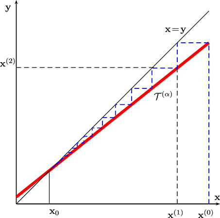
Figure 1. Fixed-point iterations for a contractive mapping ${{T}}^{(\alpha )}$ with the unique fixed point x₀.

Let us now work out the iterations (16) more explicitly by inserting the expression (14) for the operator ${{T}}^{(\alpha )}$. We then obtain the following equivalent representation of (16):

$\begin{array}{ll}{x}^{(k+1)}=x^{(k)}-\alpha \nabla f(x^{(k)}).& (26)\end{array}$

This iteration is nothing but plain vanilla GD using a fixed step size α [3].

Since the GD iteration (26) is precisely the fixed-point iteration (16), we can use Lemma (4) to characterize the convergence (rate) of GD. In particular, convergence of GD is ensured by choosing the step size of GD (26) such that q(α) = max{|1−Uα|, |1−Lα|} < 1. Moreover, in order to make the convergence as fast as possible we need to chose the step size α = α* which makes the contraction factor q(α) (cf. 20) as small as possible.

In Figure 2, we illustrate how the quantifies |1 − αL| and |1 − αU| evolve as the step size α (cf. 26) is varied. From Figure 2 we can easily read off the optimal choice

$\begin{array}{ll}{\alpha }^{*}=\frac{2}{L+U}& (27)\end{array}$

yielding the smallest possible contraction factor

$\begin{array}{l}{q}^{\ast }=\underset{\alpha \in [0,1]}{\min }q(\alpha )=\frac{U-L}{U+L}\stackrel{20}{=}\frac{\kappa -1}{\kappa +1}.\end{array}$

FIGURE 2

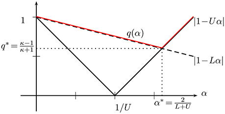
Figure 2. Dependence of contraction factor q(α) = max{|1−αL|, |1−αU|} on step size α.

We have arrived at the following characterization of GD for minimizing convex functions $f(·)\in {{S}}_n^{L,U}$.

Theorem 5. Consider the optimization problem (1) with objective function $f(·)\in {{S}}_n^{L,U}$, where the parameters L and U are fixed and known. Starting from an arbitrarily chosen initial guess x⁽⁰⁾, we construct a sequence by GD (26) using the optimal step size (27). Then,

$\begin{array}{ll}\Vert x^{(k)}-x_0\Vert \le {\left(\frac{\kappa -1}{\kappa +1}\right)}^k\Vert x^{(0)}-x_0\Vert .& (28)\end{array}$

In what follows, we will use the shorthand ${T}:={{T}}^{(\alpha *)}$ for the gradient operator ${{T}}^{(\alpha )}$ (cf. 14) obtained for the optimal step size α = α* (cf. 27).

4. First Order Methods

Without a computational model taking into account a finite amount of resources, the study of the computational complexity inherent to (1) becomes meaningless. Consider having unlimited computational resources at our disposal. Then, we could build an “optimization device” which maps each function $f(·)\in {{S}}_n^{L,U}$ to its unique minimum x₀. Obviously, this approach is infeasible since we cannot perfectly represent such a mapping, let alone its domain ${{S}}_n^{L,U}$, using a physical hardware which allows us only to handle finite sets instead of continuous spaces like ${{S}}_n^{L,U}$.

Let us further illustrate the usefulness of using a computational model in the context of machine learning from massive data sets (big data). In particular, as we have seen in the previous section, the regularized linear regression model (3) amounts to minimizing a convex quadratic function (8) with the particular choices (12). Even for this most simple machine learning model, it is typically infeasible to have access to a complete description of the objective function (8).

Indeed, in order to fully specify the quadratic function in (8), we need to fully specify the matrix Q ∈ ℝ^n×n and the vector q ∈ ℝⁿ. For the (regularized) linear regression model (3) this would require to compute Q_LR (cf. 12) from the training data ${X}={\left\{{\text{z}}^{(i)}\right\}}_{i=1}^N$. Computing the matrix Q_LR in a naive way, i.e., without exploiting any additional structure, amounts to a number of arithmetic operations on the order of N · n². This might be prohibitive in a typical big data application with N and n being on the order of billions and using distributed storage of the training data ${X}$ [12].

There has emerged a widely accepted computational model for convex optimization which abstracts away the details of the computational (hard- and software) infrastructure. Within this computational model, an optimization method for solving (1) is not provided with a complete description of the objective function, but rather it can access the objective function only via an “oracle” [2, 13].

We might think of an oracle model as an application programming interface (API), which specifies the format of queries which can be issued by a convex optimization method executed on an application layer (cf. Figure 3). There are different types of oracle models but one of the most popular type (in particular for big data applications) is a first order oracle [13]. Given a query point x ∈ ℝⁿ, a first order oracle returns the gradient ∇f(x) of the objective function at this particular point.

FIGURE 3

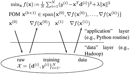
Figure 3. Programming model underlying a FOM.

A first order method (FOM) aims at solving (1) by sequentially querying a first order oracle, at the current iterate x^(k), to obtain the gradient ∇f(x^(k)) (cf. Figure 3). Using the current and past information obtained from the oracle, a FOM then constructs the new iterate x^{(k + 1)} such that eventually ${\lim }_{k\to \infty }{x}^{(k)}=x_0$. For the sake of simplicity and without essential loss in generality, we will only consider FOMs whose iterates x^(k) satisfy [13]

$\begin{array}{ll}{x}^{(k)}\in \text{span}\{x^{(0)},\nabla f(x^{(0)}),\dots ,\nabla f(x^{(k-1)})\}.& (29)\end{array}$

5. Lower Bounds on Number of Iterations

According to Section (3), solving (1) can be accomplished by the simple GD iterations (26). The particular choice α* (27) for the step size α in (26) ensures the convergence rate ${\left(\frac{\kappa -1}{\kappa +1}\right)}^k$ with the condition number κ = U/L of the function class ${{S}}_n^{L,U}$. While this convergence is quite fast, i.e., the error decays exponentially with iteration number k, we would, of course, like to know how efficient this method is in general.

As detailed in Section (4), in order to study the computational complexity and efficiency of convex optimization methods, we have to define a computational model such as those underlying FOMs (cf. Figure 3). The next result provides a fundamental lower bound on the convergence rate of any FOM (cf. 29) for solving (1).

Theorem 6. Consider a particular FOM, which for a given convex function $f(·)\in {{S}}_n^{L,U}$ generates iterates x^(k) satisfying (29). For fixed L, U there is a sequence of functions $f_n(·)\in {{S}}_n^{L,U}$ (indexed by dimension n) such that

$\begin{array}{ll}\Vert x^{(k)}-x_0\Vert \ge \Vert x^{(0)}-x_0\Vert \frac{1-1/\sqrt{\kappa }}{1+\sqrt{\kappa }}{\left(\frac{\sqrt{\kappa }-1}{\sqrt{\kappa }+1}\right)}^k-|\delta (n)|& (30)\end{array}$

with a sequence δ(n) such that ${\lim }_{n\to \infty }|\delta (n)|=0$.

Proof. see Section (8.1).□

There is a considerable gap between the upper bound (28) on the error achieved by GD after k iterations and the lower bound (30) which applies to any FOM which is run for the same number iterations. In order to illustrate this gap, we have plotted in Figure 4 the upper and lower bound for the (quite moderate) condition number κ = 100.

FIGURE 4

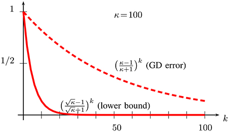
Figure 4. Upper bound (28) on convergence rate of GD and lower bound (30) on convergence rate for any FOM minimizing functions $f(·)\in {{S}}_n^{L,U}$ with condition number κ = U/L = 100.

Thus, there might exist a FOM which converges faster than the GD method (28) and comes more close to the lower bound (30). Indeed, in the next section, we will detail how to obtain an accelerated FOM by applying a fixed point preserving transformation to the operator ${T}$ (cf. 16), which is underlying the GD method (26). This accelerated gradient method is known as the heavy balls (HB) method [14] and effectively achieves the lower bound (30), i.e., the HB method is already optimal among all FOM's for solving (1) with an objective function $f(·)\in {{S}}_n^{L,U}$.

6. Accelerating Gradient Descent

Let us now show how to modify the basic GD method (26) in order to obtain an accelerated FOM, whose convergence rate essentially matches the lower bound (30) for the function class ${{S}}_n^{L,U}$ with condition number κ = U/L>1 (cf. 7) and is therefore optimal among all FOMs.

Our derivation of this accelerated gradient method, which is inspired by the techniques used in Ghadimi et al. [15], starts from an equivalent formulation of GD as the fixed-point iteration

$\begin{array}{ll}{\overline{x}}^{(k)}=\overline{{T}}{\overline{x}}^{(k-1)}& (31)\end{array}$

with the operator

$\begin{array}{ll}\overline{{T}}:{ℝ}^{2n}\to {ℝ}^{2n}:\left(\begin{array}{c}u\\ v\end{array}\right)\mapsto \left(\begin{array}{c}u-\alpha \nabla u\\ u\end{array}\right)=\left(\begin{array}{c}{T}u\\ u\end{array}\right).& (32)\end{array}$

As can be verified easily, the fixed-point iteration (31) starting from an arbitrary initial guess ${\overline{x}}^{\left(0\right)}=\left(\begin{array}{c}{z}^{\left(0\right)}\\ y^{\left(0\right)}\end{array}\right)$ is related to the GD iterate x^(k) (cf. 26), using initial guess z⁽⁰⁾, as

$\begin{array}{ll}{\overline{x}}^{(k)}=\left(\begin{array}{c}{x}^{(k)}\\ x^{(k-1)}\end{array}\right)& (33)\end{array}$

for all iterations k ≥ 1.

By the equivalence (33), Theorem (5) implies that for any initial guess ${\bar{\text{x}}}^{(0)}$ the iterations (31) converge to the fixed point

$\begin{array}{ll}{\overline{x}}_0:=\left(\begin{array}{c}{x}_0\\ x_0\end{array}\right)\in {ℝ}^{2n}& (34)\end{array}$

with x₀ being the unique minimizer of $f(·)\in {{S}}_n^{L,U}$. Moreover, the convergence rate of the fixed-point iterations (31) is precisely the same as those of the GD method, i.e., governed by the decay of ${\left(\frac{\kappa -1}{\kappa +1}\right)}^k$, which is obtained for the optimal step size α = α* (cf. 27).

We will now modify the operator $\overline{{T}}$ in (32) to obtain a new operator ${M}:{ℝ}^{2n}\to {ℝ}^{2n}$ which has the same fixed points (34) but improved contraction behavior, i.e., the fixed point iteration

$\begin{array}{ll}{\tilde{x}}^{(k)}={M}{\tilde{x}}^{(k-1)},& (35)\end{array}$

will converge faster than those obtained from $\overline{{T}}$ in (31) (cf. Figure 5). In particular, this improved operator ${M}$ is defined as

$\begin{array}{ll}{M}:{ℝ}^{2n}\to {ℝ}^{2n}:\left(\begin{array}{c}u\\ v\end{array}\right)\mapsto \left(\begin{array}{c}u-\tilde{\alpha }\nabla u+\tilde{\beta }(u-v)\\ u\end{array}\right),& (36)\end{array}$

with

$\begin{array}{ll}\tilde{\alpha }:=\frac{4}{{(\sqrt{U}+\sqrt{L})}^2},\text{and }\tilde{\beta }:={\left[\frac{\sqrt{U}-\sqrt{L}}{\sqrt{U}+\sqrt{L}}\right]}^2.& (37)\end{array}$

FIGURE 5

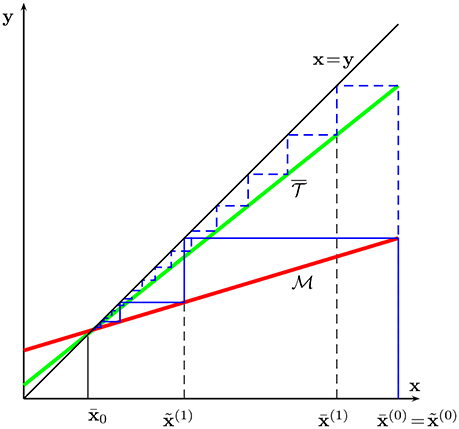
Figure 5. Schematic illustration of the fixed-point iteration using operator $\overline{{T}}$ (32) (equivalent to GD) and for the modified operator ${M}$ (36) (yielding HB method).

As can be verified easily, the fixed point ${\left(x_0^T,x_0^T\right)}^T$ of $\overline{{T}}$ is also a fixed point of ${M}$.

Before we analyze the convergence rate of the fixed-point iteration (35), let us work out explicitly the FOM which is represented by the fixed-point iteration (35). To this end, we partition the kth iterate, for k ≥ 1, as

$\begin{array}{ll}{\tilde{x}}^{(k)}:=\left(\begin{array}{c}{x}_{\text{HB}}^{(k)}\\ x_{\text{HB}}^{(k-1)}\end{array}\right).& (38)\end{array}$

Inserting (38) into (35), we have for k ≥ 1

$\begin{array}{ll}{x}_{\text{HB}}^{(k)}=x_{\text{HB}}^{(k-1)}-\tilde{\alpha }\nabla f(x_{\text{HB}}^{(k-1)})+\tilde{\beta }(x_{\text{HB}}^{(k-1)}-x_{\text{HB}}^{(k-2)})& (39)\end{array}$

with the convention ${\text{x}}_{\text{HB}}^{(-1)}:=0$. The iteration (39) defines the HB method [14] for solving the optimization problem (1). As can be verified easily, like the GD method, the HB method is a FOM. However, contrary to the GD iteration (26), the HB iteration (39) also involves the penultimate iterate ${\text{x}}_{\text{HB}}^{(k-2)}$ for determining the new iterate ${\text{x}}_{\text{HB}}^{(k)}$.

We will now characterize the converge rate of the HB method (39) via its fixed-point equivalent (35). To this end, we restrict ourselves to the subclass of ${{S}}_n^{L,U}$ given by quadratic functions of the form (8).

Theorem 7. Consider the optimization problem (1) with objective function $f(·)\in {{S}}_n^{L,U}$ which is a quadratic (26). Starting from an arbitrarily chosen initial guess ${\text{x}}_{\text{HB}}^{(-1)}$ and ${\text{x}}_{\text{HB}}^{(0)}$, we construct a sequence ${\text{x}}_{\text{HB}}^{(k)}$ via iterating (27). Then,

$\begin{array}{ll}\Vert x_{\text{HB}}^{(k)}-x_0\Vert \le C(\kappa )k{(\frac{\sqrt{\kappa }-1}{\sqrt{\kappa }+1})}^k(\Vert x_{\text{HB}}^{(0)}-x_0\Vert +\Vert x_{\text{HB}}^{(-1)}-x_0\Vert ).& (40)\end{array}$

with

$\begin{array}{l}C(\kappa ):=4(2+2\tilde{\beta }+\tilde{\alpha })\frac{\sqrt{\kappa }+1}{\sqrt{\kappa }-1}.\end{array}$

Proof. see Section (8.2).□

The upper bound (40) differs from the lower bound (30) by the factor k. However, the discrepancy is rather decent as this linear factor in (40) grows much slower than the exponential ${\left(\frac{\sqrt{\kappa }-1}{\sqrt{\kappa }+1}\right)}^k$ in (40) decays. In Figure 6, we depict the upper bound (40) on the error of the HB iterations (39) along with the upper bound (28) on the error of the GD iterations (26) and the lower bound (30) on the error of any FOM after k iterations.

FIGURE 6

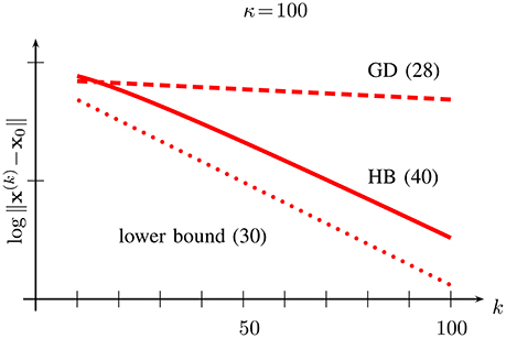
Figure 6. Dependence on iteration number k of the upper bound (40) on error of HB (solid), upper bound (28) for error of GD (dashed) and lower bound (30) (dotted) for FOMs for the function class ${{S}}_n^{L,U}$ with condition number κ = U/L = 100.

We highlight that, strictly speaking, the bound (40) only applies to a subclass of smooth strongly convex functions $f(·)\in {{S}}_n^{L,U}$, i.e., it applies only to quadratic functions of the form (8). However, as discussed in Section (2), given a particular point x, we can approximate an arbitrary function $f(·)\in {{S}}_n^{L,U}$ with a quadratic function $\tilde{f}(\text{x})$ of the form (8). The approximation error ε(x) (cf. (11)) will be small for all points x sufficiently close to x₀. Making this reasoning more precise and using well-known results on fixed-point iterations with inexact updates [6], one can verify that the bound (40) essentially applies to any function $f(·)\in {{S}}_n^{L,U}$.

7. Conclusions

We have presented a fixed-point theory of some basic gradient methods for minimizing convex functions. The approach via fixed-point theory allows for a rather elegant analysis of the convergence properties of these gradient methods. In particular, their convergence rate is obtained as the contraction factor for an operator associated with the objective function.

The fixed-point approach is also appealing since it leads rather naturally to the acceleration of gradient methods via fixed-point preserving transformations of the underlying operator. We plan to further develop the fixed-point theory of gradient methods in order to accommodate stochastic variants of GD such as SGD. Furthermore, we can bring the popular class of proximal methods into the picture by replacing the gradient operator underlying GD with the proximal operator.

However, by contrast to FOMs (such as the GD method), proximal methods use a different oracle model (cf. Figure 3). In particular, proximal methods require an oracle which can evaluate the proximal mapping efficiently which is typically more expensive than gradient evaluations. Nonetheless, the popularity of proximal methods is due to the fact that for objective functions arising in many important machine learning applications, the proximal mapping can be evaluated efficiently.

8. Proofs of Main Results

In this section we present the (somewhat lengthy) proofs for the main results stated in Sections (5) and (6).

8.1. Proof of Theorem (6)

Without loss of generality we consider FOM which use the initial guess x⁽⁰⁾ = 0. Let us now construct a function $f_n(·)\in {{S}}_n^{L,U}$ which is particularly difficult to optimize by a FOM (cf. 29) such as the GD method (26). In particular, this function is the quadratic

$\begin{array}{ll}\widehat{f}(x):=(1/2)x^{T}Px+{\tilde{q}}^{T}x& (41)\end{array}$

with vector

$\begin{array}{ll}\tilde{q}:=\frac{L(\kappa -1)}{4}{(1,0,\dots ,0)}^T\in {ℝ}^n& (42)\end{array}$

and matrix

$\begin{array}{ll}P:=(L/4)(\kappa -1)\tilde{Q}+LI\in {ℝ}^{n\times n}.& (43)\end{array}$

The matrix $\tilde{\text{Q}}$ is defined row-wise by successive circular shifts of its first row

$\begin{array}{ll}\tilde{q}:={(2,-1,0,\dots ,0,-1)}^T\in {ℝ}^n.& (44)\end{array}$

Note that the matrix P in (43) is a circulant matrix [16] with orthonormal eigenvectors ${\left\{u^{(l)}\right\}}_{l=1}^n$ given element-wise as

$\begin{array}{ll}{u}_i^{(l)}=(1/\sqrt{n})\exp (j2\pi (i-1)(l-1)/n).& (45)\end{array}$

The eigenvalues λ_l(P) of the circulant matrix P are obtained as the discrete Fourier transform (DFT) coefficients of its first row [16]

$\begin{array}{ll}\begin{array}{l}p=\frac{L(\kappa -1)}{4}\tilde{q}+L{e}_1^T\hfill \\ \stackrel{(44)}{=}\frac{L(\kappa -1)}{4}(2,-1,0,\dots ,0,-1)+L{\left(1,0,\dots ,0\right)}^T,\hfill \end{array}& (46)\end{array}$

i.e.,

$\begin{array}{l}{\lambda }_l(P)={\displaystyle \sum _{i=1}^n{p}_i}\exp (-j2\pi (i-1)(l-1)/n)\\ \stackrel{(46)}{=}(L/2)(\kappa -1)(1-\cos (-2\pi (i-1)/n)+L.& (47)\end{array}$

Thus, λ_l(P) ∈ [L, U] and, in turn, $f_n(·)\in {{S}}_n^{L,U}$ (cf. 6).

Consider the sequence x^(k) generated by some FOM, i.e., which satisfies (29), for the particular objective function f_n(x) (cf. 41) using initial guess x₀ = 0. It can be verified easily that the kth iterate x^(k) has only zero entries starting from index k + 1, i.e.,

$\begin{array}{l}{x}_l^{(k)}=0\text{ for all }l\in \{k+1,\dots ,n\}.\end{array}$

This implies

$\begin{array}{ll}\Vert x^{(k)}-x_0\Vert \ge |x_{0,k+1}|.& (48)\end{array}$

The main part of the proof is then to show that the minimizer x₀ for the particular function f_n(·) cannot decay too fast, i.e., we will derive a lower bound on |x_0,k+1|.

Let us denote the DFT coefficients of the finite length discrete time signal represented by the vector $\tilde{\text{q}}$ as

$\begin{array}{l}{c}_l={\displaystyle \sum _{i=1}^n{\tilde{q}}_i}\exp (-j2\pi (i-1)l/n)\\ \stackrel{(42)}{=}(L/4)(\kappa -1).& (49)\end{array}$

Using the optimality condition (13), the minimizer for (41) is

$\begin{array}{ll}{x}_0=-P^{-1}\tilde{q}.& (50)\end{array}$

Inserting the spectral decomposition $P={\displaystyle \sum _{l=1}^n{\lambda }_l{u}^{(l)}{\left(u^{(l)}\right)}^H}$ [16, Theorem 3.1] of the psd matrix P into (50),

$\begin{array}{l}{x}_{0,k}=-{\left(P^{-1}\tilde{q}\right)}_k\\ \stackrel{(45)}{=}-(1/n){\displaystyle {\displaystyle \sum }_{i=1}^n}(c_i/{\lambda }_i)\exp (j2\pi (i-1)(k-1)/n)\hfill \\ \stackrel{(47),(49)}{=}-\frac{1}{n}{\displaystyle {\displaystyle \sum }_{i=1}^n}\frac{\exp (j2\pi (i-1)(k-1)/n)}{2(1-\cos (-2\pi (i-1)/n))+4/(\kappa -1)}.\hfill & (51)\end{array}$

We will also need a lower bound on the norm ‖x₀‖ of the minimizer of f_n(·). This bound can be obtained from (50) and λ_l(P) ∈ [L, U], i.e., ${\lambda }_l\left(P^{-1}\right)\in [1/U,1/L]$,

$\begin{array}{ll}\Vert x_0\Vert \le (1/L)\Vert \tilde{q}\Vert \stackrel{(42)}{=}\frac{\kappa -1}{4}.& (52)\end{array}$

The last expression in (51) is a Riemann sum for the integral $\underset{\theta =0}{\overset{1}{\int }}\frac{exp(-j2\pi \theta )}{2(1-exp(-j2\pi \theta ))+4/(\kappa -1)}d\theta$. Indeed, by basic calculus [10, Theorem 6.8]

$\begin{array}{ll}{x}_{0,k}=-{\displaystyle \underset{\theta =0}{\overset{1}{\int }}\frac{\exp (j2\pi (k-1)\theta )}{2(1-\cos (2\pi \theta ))+4/(\kappa -1)}}d\theta +\delta (n)& (53)\end{array}$

where the error δ(n) becomes arbitrarily small for sufficiently large n, i.e., $\underset{n\to \infty }{lim}|\delta (n)|=0$.

According to Lemma (9),

$\begin{array}{l}{\displaystyle \underset{\theta =0}{\overset{1}{\int }}\frac{\exp (j2\pi (k-1)\theta )}{2(1-\cos (2\pi \theta ))+4/(\kappa -1)}}d\theta =\frac{\kappa -1}{4\sqrt{\kappa }}{(\frac{\sqrt{\kappa }-1}{\sqrt{\kappa }+1})}^k,\end{array}$

which, by inserting into (53), yields

$\begin{array}{ll}{x}_{0,k}=-\frac{\kappa -1}{4\sqrt{\kappa }}{(\frac{\sqrt{\kappa }-1}{\sqrt{\kappa }+1})}^k+\delta (n).& (54)\end{array}$

Putting together the pieces,

$\begin{array}{l}\begin{array}{l}\Vert x^{(k)}-x_0\Vert \stackrel{(48)}{\ge }|x_{0,k+1}|\hfill \\ \stackrel{(54)}{\ge }\frac{\kappa -1}{4\sqrt{\kappa }}\left(\frac{\sqrt{\kappa }-1}{\sqrt{\kappa }+1}\right){\left(\frac{\sqrt{\kappa }-1}{\sqrt{\kappa }+1}\right)}^k-|\delta (n)|\hfill \\ \stackrel{(52)}{\ge }\Vert x_0\Vert \frac{1-1/\sqrt{\kappa }}{1+\sqrt{\kappa }}{\left(\frac{\sqrt{\kappa }-1}{\sqrt{\kappa }+1}\right)}^k-|\delta (n)|\hfill \\ \stackrel{x^{(0)}=0}{=}\Vert x^{(0)}-x_0\Vert \frac{1-1/\sqrt{\kappa }}{1+\sqrt{\kappa }}{\left(\frac{\sqrt{\kappa }-1}{\sqrt{\kappa }+1}\right)}^k-|\delta (n)|.\hfill \end{array}\end{array}$

8.2. Proof of Theorem (7)

By evaluating the operator ${M}$ (cf. 36) for a quadratic function f(·) of the form (8), we can verify

$\begin{array}{ll}Mx-My=R(x-y)& (55)\end{array}$

with the matrix

$\begin{array}{ll}R=\left(\begin{array}{cc}(1+\tilde{\beta })I-\tilde{\alpha }Q& -\tilde{\beta }I\\ I& 0\end{array}\right).& (56)\end{array}$

This matrix R ∈ ℝ^2n×2n is a 2 × 2 block matrix whose individual blocks can be diagonalized simultaneously via the orthonormal eigenvectors U = (u⁽¹⁾, …, u⁽ⁿ⁾) of the psd matrix Q. Inserting the spectral decomposition $\text{Q}=\text{U}\text{diag}{\left\{{\lambda }_i\right\}}_{i=1}^n{\text{U}}^H$ into (56),

$\begin{array}{ll}R=UPB{P}^H{U}^H,& (57)\end{array}$

with some (orthonormal) permutation matrix P and a block diagonal matrix

$\begin{array}{ll}B:=\left(\begin{array}{ccc}{B}^{(1)}& \dots & 0\\ 0& \ddots & ⋮\\ 0& \dots & B^{(n)}\end{array}\right),B^{(i)}:=\left(\begin{array}{cc}1+\tilde{\beta }-\tilde{\alpha }{\lambda }_i& -\tilde{\beta }\\ 1& 0\end{array}\right).& (58)\end{array}$

Combining (57) with (55) and inserting into (35) yields

$\begin{array}{ll}{\tilde{x}}^{(k)}-{\tilde{x}}_0=UP{B}^k{P}^H{U}^H({\tilde{x}}^{(0)}-{\tilde{x}}_0).& (59)\end{array}$

In order to control the convergence rate of the iterations (35), i.e., the decay of the error $\Vert {\tilde{\text{x}}}^{(k)}-{\tilde{\text{x}}}_0\Vert$, we will now derive an upper bound on the spectral norm of the block diagonal matrix B^k (cf. 58).

Due to the block diagonal structure (58), we can control the norm of B^k via controlling the norm of the powers of its diagonal blocks (B⁽ⁱ⁾)^k since

$\begin{array}{ll}\Vert B^k\Vert =\underset{i}{\max }\Vert {(B^{(i)})}^k\Vert .& (60)\end{array}$

A pen and paper exercise reveals

$\begin{array}{ll}\rho (B^{(i)})={\tilde{\beta }}^{1/2}\stackrel{(37)}{=}\frac{\sqrt{U}-\sqrt{L}}{\sqrt{U}+\sqrt{L}}=\frac{\sqrt{\kappa }-1}{\sqrt{\kappa }+1}.& (61)\end{array}$

Combining (61) with Lemma (8) yields

$\begin{array}{ll}{(B^{(i)})}^k=\left(\begin{array}{cc}{\lambda }_1^k& d\\ 0& {\lambda }_2^k\end{array}\right),& (62)\end{array}$

with $\left|{\lambda }_1\right|,\left|{\lambda }_2\right|\le {\tilde{\beta }}^{1/2}$ and $d\le k(2+2\tilde{\beta }+\tilde{\alpha }){\tilde{\beta }}^{(k-1)/2}$. Using the shorthand $\tilde{c}:=(2+2\tilde{\beta }+\tilde{\alpha })$, we can estimate the spectral norm of B^k as

$\begin{array}{l}\Vert B^k\Vert \stackrel{(60)}{=}\underset{i}{\max }\Vert {\left(B^{\left(i\right)}\right)}^k\Vert \\ \stackrel{(62)}{\le }{\left(\frac{\sqrt{\kappa }-1}{\sqrt{\kappa }+1}\right)}^k\left(1+k\tilde{c}\frac{\sqrt{\kappa }+1}{\sqrt{\kappa }-1}\right).& (63)\end{array}$

Combining (63) with (59),

$\begin{array}{ll}\begin{array}{l}\Vert {\tilde{x}}^{(k)}-{\tilde{x}}_0\Vert \le {\left(\frac{\sqrt{\kappa }-1}{\sqrt{\kappa }+1}\right)}^k\left(1+k\tilde{c}\frac{\sqrt{\kappa }+1}{\sqrt{\kappa }-1}\right)\Vert {\tilde{x}}^{(0)}-{\tilde{x}}_0\Vert \hfill \\ \stackrel{\tilde{c}\ge 1}{\le }2k\tilde{c}\frac{\sqrt{\kappa }+1}{\sqrt{\kappa }-1}{\left(\frac{\sqrt{\kappa }-1}{\sqrt{\kappa }+1}\right)}^k\Vert {\tilde{x}}^{(0)}-{\tilde{x}}_0\Vert .\hfill \end{array}& (64)\end{array}$

Using (38), the error bound (64) can be translated into an error bound on the HB iterates ${\text{x}}_{\text{HB}}^{(k)}$, i.e.,

$\begin{array}{l}\begin{array}{l}\Vert x_{HB}^{(k)}-x_0\Vert \le \hfill \\ 4k\tilde{c}\frac{\sqrt{\kappa }+1}{\sqrt{\kappa }-1}{\left(\frac{\sqrt{\kappa }-1}{\sqrt{\kappa }+1}\right)}^k(\Vert x_{HB}^{(0)}-x_0\Vert +\Vert x_{HB}^{(-1)}-x_0\Vert ).\hfill \end{array}\end{array}$

9. Technicalities

We collect some elementary results from linear algebra and analysis, which are required to prove our main results.

Lemma 8. Consider a matrix M = $\left(\begin{array}{cc}a& b\\ 1& 0\end{array}\right)$ ∈ ℝ^2×2 with spectral radius ρ(M). Then, there is an orthonormal matrix U ∈ ℂ^2×2 such that

$\begin{array}{ll}{M}^k=U\left(\begin{array}{cc}{\lambda }_1^k& d\\ 0& {\lambda }_2^k\end{array}\right)U^{H}fork\in \mathbb{N},& (65)\end{array}$

where |λ₁|, |λ₂| ≤ ρ(M) and |d|(|a| + |b| + 1)ρ^k−1(M).

Proof. Consider an eigenvalue λ₁ of the matrix M with normalized eigenvector $\text{u}={(u_1,u_2)}^H$, i.e., Mu = λ₁u with ‖u‖ = 1. According to Golub and Van Loan [11, Lemma 7.1.2], we can find a normalized vector $\text{v}={(v_1,v_2)}^H$, orthogonal to u, such that

$\begin{array}{ll}M=(u,v)\left(\begin{array}{cc}{\lambda }_1& d\\ 0& {\lambda }_2\end{array}\right){(u,v)}^H,& (66)\end{array}$

or equivalently

$\begin{array}{ll}\left(\begin{array}{cc}{\lambda }_1& d\\ 0& {\lambda }_2\end{array}\right)={(u,v)}^{H}M(u,v),& (67)\end{array}$

with some eigenvalue λ₂ of M. As can be read off (67), d = u₁(u₂a + v₂b) + v₁u₂ which implies (65) since |u₁|, |u₂|, |v₁|, |v₂| ≤ 1. Based on (66), we can verify (65) by induction.□

Lemma 9. For any κ > 1 and k ∈ ℕ,

$\begin{array}{ll}{\displaystyle \underset{\theta =0}{\overset{1}{\int }}\frac{\exp (j2\pi (k-1)\theta )}{2(1-\cos (2\pi \theta ))+4/(\kappa -1)}}d\theta =\frac{\kappa -1}{4\sqrt{\kappa }}{(\frac{\sqrt{\kappa }-1}{\sqrt{\kappa }+1})}^k.& (68)\end{array}$

Proof. Let us introduce the shorthand z := exp(j2πθ) and further develop the LHS of (68) as

$\begin{array}{l}{\displaystyle \underset{\theta =0}{\overset{1}{\int }}\frac{z^{k-1}}{2(1-(z^{-1}+z)/2)+4/(\kappa -1)}}d\theta \\ ={\displaystyle \underset{\theta =0}{\overset{1}{\int }}\frac{z^k}{2(z-(1+z^2)/2)+4z/(\kappa -1)}}d\theta .& (69)\end{array}$

The denominator of the integrand in (69) can be factored as

$\begin{array}{ll}2(z-(1+z^2)/2)+4z/(\kappa -1)=-(z-z_1)(z-z_2)& (70)\end{array}$

with

$\begin{array}{ll}{z}_1:=\frac{\sqrt{\kappa }+1}{\sqrt{\kappa }-1},\text{and }{z}_2:=\frac{\sqrt{\kappa }-1}{\sqrt{\kappa }+1}.& (71)\end{array}$

Inserting (70) into (69),

$\begin{array}{l}{\displaystyle \underset{\theta =0}{\overset{1}{\int }}\frac{z^k}{2(z-(1+z^2)/2)+4/(\kappa -1)}}d\theta \\ =-{\displaystyle \underset{\theta =0}{\overset{1}{\int }}\frac{z^k}{(z-z_1)(z-z_2)}}d\theta \\ ={\displaystyle \underset{\theta =0}{\overset{1}{\int }}-}\frac{z^k{(z_1-z_2)}^{-1}}{z-z_1}+\frac{z^k{(z_1-z_2)}^{-1}}{z-z_2}d\theta .& (72)\end{array}$

Since |z₂| < 1, we can develop the second term in (72) by using the identity [17, Section 2.7]

$\begin{array}{ll}{\displaystyle \underset{\theta =0}{\overset{1}{\int }}\frac{\exp (j2\pi k\theta )}{\exp (j2\pi \theta )-\alpha }}d\theta ={\alpha }^{k-1}\text{for}k\in \mathbb{N},\alpha \in ℝ,|\alpha |<1.& (73)\end{array}$

Since |z₁|>1, we can develop the first term in (72) by using the identity [17, Section 2.7]

$\begin{array}{ll}{\displaystyle \underset{\theta =0}{\overset{1}{\int }}\frac{\exp (j2\pi k\theta )}{\exp (j2\pi \theta )-\alpha }}d\theta =0\text{ for }k\in \mathbb{N},\alpha \in ℝ,|\alpha |>1.& (74)\end{array}$

Applying (73) and (74) to (72),

$\begin{array}{ll}{\displaystyle \underset{\theta =0}{\overset{1}{\int }}\frac{z^k}{2(z-(1+z^2)/2)+4/(\kappa -1)}}d\theta =\frac{z_2^{k-1}}{z_1-z_2}.& (75)\end{array}$

Inserting (75) into (69), we arrive at

$\begin{array}{ll}{\displaystyle \underset{\theta =0}{\overset{1}{\int }}\frac{\exp (j2\pi (k-1)\theta )}{2(1-\cos (2\pi \theta ))+4/(\kappa -1)}}d\theta =\frac{z_2^{k-1}}{z_1-z_2}.& (76)\end{array}$

The proof is finished by combining (76) with the identity

$\begin{array}{l}\frac{1}{z_1-z_2}\stackrel{\left(71\right)}{=}\frac{\sqrt{\kappa }+1}{\sqrt{\kappa }-1}-\frac{\sqrt{\kappa }-1}{\sqrt{\kappa }+1}=\frac{4\sqrt{\kappa }}{\kappa -1}.\end{array}$

     □

Author Contributions

The author confirms being the sole contributor of this work and approved it for publication.

Conflict of Interest Statement

The author declares that the research was conducted in the absence of any commercial or financial relationships that could be construed as a potential conflict of interest.

Acknowledgments

This paper is a wrap-up of the lecture material created for the course Convex Optimization for Big Data over Networks, taught at Aalto University in spring 2017. The student feedback on the lectures has been a great help to develop the presentation of the contents. In particular, the detailed feedback of students Stefan Mojsilovic and Matthias Grezet on early versions of the paper is appreciated sincerely.

References

1. Bottou L, Bousquet O. The tradeoffs of large scale learning. In: Advances in Neural Information Processing Systems (NIPS). Vancouver, BC (2008). p. 161–8.

Google Scholar

2. Cevher V, Becker S, Schmidt M. Convex optimization for big data: scalable, randomized, and parallel algorithms for big data analytics. IEEE Signal Process Mag. (2014) 31:32–43. doi: 10.1109/MSP.2014.2329397

CrossRef Full Text | Google Scholar

3. Goodfellow I, Bengio Y, Courville A. Deep Learning. Cambridge, MA: MIT Press (2016).

Google Scholar

4. Walker HF, Ni P. Anderson acceleration for fixed-point iterations. SIAM J Numer Anal. (2011) 49:1715–35. doi: 10.1137/10078356X

CrossRef Full Text | Google Scholar

5. Birken P. Termination criteria for inexact fixed-point schemes. Num Lin Alg App. (2015) 22:702–16. doi: 10.1002/nla.1982

CrossRef Full Text | Google Scholar

6. Alfeld P. Fixed point iteration with inexact function values. Math Comput. (1982) 38:87–98. doi: 10.1090/S0025-5718-1982-0637288-5

CrossRef Full Text | Google Scholar

7. Boyd S, Vandenberghe L. Convex Optimization. Cambridge: Cambridge University Press (2004). doi: 10.1017/CBO9780511804441

PubMed Abstract | CrossRef Full Text | Google Scholar

8. Bishop CM. Pattern Recognition and Machine Learning. New York, NY: Springer (2006).

Google Scholar

9. Bauschke HH, Combettes PL. Convex Analysis and Monotone Operator Theory in Hilbert Spaces. New York, NY: Springer (2010).

Google Scholar

10. Rudin W. Principles of Mathematical Analysis, 3rd Edn. New York, NY: McGraw-Hill (1976).

11. Golub GH, Van Loan CF. Matrix Computations, 3rd Edn. Baltimore, MD: Johns Hopkins University Press (1996).

12. Giannakis GB, Slavakis K, Mateos G. Signal processing for big data. In: Tutorial at EUSIPCO. Lisabon (2014).

Google Scholar

13. Nesterov Y. Introductory Lectures on Convex Optimization. vol. 87 of Applied Optimization. Boston, MA: Kluwer Academic Publishers (2004).

Google Scholar

14. Polyak BT. Some methods of speeding up the convergence of iteration methods. USSR Comput Math Math Phys. (1964) 4:1–17.

Google Scholar

15. Ghadimi E, Shames I, Johansson M. Multi-step gradient methods for networked optimization. IEEE Trans Signal Process. (2013) 61:5417–29.

Google Scholar

16. Gray RM. Toeplitz and Circulant Matrices: A review. vol. 2 of Foundations and Trends in Communications and Information Theory. Boston, MA (2006).

Google Scholar

17. Oppenheim AV, Schafer RW, Buck JR. Discrete-Time Signal Processing, 2nd Edn. Englewood Cliffs, NJ: Prentice Hall (1998).

Google Scholar