Output-Feedback Control of Virus Spreading in Complex Networks With Quarantine

1. Introduction

Studies on the propagation and control of viruses and infectious diseases in human and animal populations [1–8] have gained a great importance in the last years. Understanding and controlling spreading processes is a problem of interdisciplinary nature [9–12]. The use of mathematical and physical inspired models that give account of the dynamics of propagation of infections have gained acceptance since the London cholera epidemics in September 1853 when John Snow divided a map of London into sectors (in a way, nowadays, equiparable to a Voronoi diagram) to calculate who was most likely to use each water pump in the city and in this way, discovered that the 40 Broad Street pump was the main focus of the cholera infection.

Some decades later, McKendrick [13] and Kermack and McKendrick [14] proposed the SIR model that divides the population in three different compartments or groups of individuals: Susceptible, Infective, and Recovered (or Removed) that had the disease and become immune or died. This pioneering work gave birth to the SIS (Susceptible-Infected-Susceptible) model mainly because many diseases do not confer any immunity. Extensions such as the SIQ (Susceptible-Infected-Quarantine) model (see e.g., [15–17] ) appeared in order to account for the dynamics of the spreading of infections when quarantine has been implemented as a means to control the massive spreading of the infectious disease. Accordingly, a new class of quarantined individuals is included. These individuals are removed, with some probability from the class of infected individuals.

Although these models were proposed for modeling spreading in populations with no structure, nowadays the SIS and SIQ models have been extended to model the spreading process in a population mapped on a complex network.

In recent years, Markov-chain based models for a Susceptible-Infected-Susceptible (SIS) dynamics over complex networks have been used [4–8, 18] to describe spreading processes in networks. Using these models, it is possible to determine the macroscopic properties of the system as well as the description of the dynamics of individual nodes. One interesting result is that the calculated infection threshold depends on the value of the spectral radius of the adjacency matrix, thus relating the network structure with spreading behavior.

In the present work we will study the spreading of diseases using a Markov-chain based model for a Susceptible-Infected-Quarentine (SIQ) dynamics over a complex network that has been used in a simplified version for the determination of stability tresholds in recent studies by the authors [15, 17]. We will show that, even when the built-in control strategy of quarantine is not able to ensure virus extinction, it is always possible to solve the problem of epidemic spreading extinction. In order to accomplish this task, we determine sufficient conditions for stabilizing the extinction state in a complex network of arbitrary topology. One remarkable point is that, these conditions give a clue to identify the nodes that do not need any control to reach the extinction state and distinguish them from the nodes that need to be controlled. Inspired on the ideas of control theory, the set of nodes that do not need to be controlled (in order to reach the extinction state) will be associated with the zero dynamics of the system [19, 20]. At the same time, the set of nodes to be monitored and controlled will be identified and a decentralized feedback control will be applied in order to stabilize the extinction state. Accordingly, it is proven that the extinction state is an exponentially stable fixed point for the zero dynamics.

We have performed numerical simulations using a scale-free complex network with 1 million nodes constructed as proposed by Barabasi [21] and found a complete agreement of the numerical results with our theoretical findings.

The paper is organized as follows: section Methods presents the problem statement for the SIQ model mapped on a complex network of arbitrary topology and the control problem we want to solve together with some definitions. In section Results, sufficient conditions for the stabilization of the extinction state are derived. Using these conditions we establish a selection criterion that allows to identify the set of nodes that need to be controlled in order to reach the extinction state. Afterwards, we design a simple stabilizing output-feedback control and present our simulation results. In section Discussion and Conclusions we summarize our main results and present our main conclusions.

2. Methods

As pointed out in the introduction, the SIQ model belongs to a class of models that are used to capture possible human interactions employed to impede the spreading of an infection process and it is essentially an extension of the SIS model in which the model and control strategies are co-developed to yield a kind of closed-loop control model [22]. In order to reveal the dynamics and essential mechanisms of this model, we proceed to (i) formulate the SIQ model in a complex network (ii) introduce the specific control problem.

2.1 The SIQ Model in a Complex Network

Consider a network of N nodes described by an undirected graph G(V, E) of any topology. Let V = {v₁, v₂, …, v_N} being the set of nodes and E = {e_{i, j}} the set of connecting edges. The adjacency matrix associated to G(V, E) is given by A = {a_ij}, where a_ij = 1 if e_{i, j} ∈ E and zero otherwise. The set of neighbor nodes of a node v_i ∈ V is defined as

$\begin{array}{cc}\begin{array}{r}{V}_i=\left\{v_j\in V|a_{ij}=a_{ji}=1\right\}\subset V,\end{array}& (1)\end{array}$

and the number of neighbors or degree of a node v_i is given by ${{N}}_i=\left|V_i\right|$.

As formulated in Bernal Jaquez et al. [15], the underlying process for every node is depicted in Figure 1, as a discrete time Markov process. A node v_i can be in state I (Infected) with probability p_i(t), in state Q (Quarantine) with probability q_i(t), or in state S (Susceptible) with probability s_i(t) = 1 − p_i(t) − q_i(t). At each time step, the probability functions p_i(t), s_i(t) are updated due to the fact that every node can transit from state S to state I with probability 1−ζ_i or from state I to state Q with probability τ_i and from state Q to state S with probability μ_i because nodes are interacting.

FIGURE 1

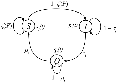
Figure 1. State transition diagram for each node v_i ∈ V. The states Infected, Quarantine and Susceptible are represented by I, Q, and S, respectively.

According to the transition diagram shown in Figure 1, we have the following dynamical system:

$\begin{array}{cc}\begin{array}{l}\begin{array}{c}{p}_i(t+1)=(1-{\tau }_i)p_i(t)+(1-{\zeta }_i(P(t)))s_i(t),\end{array}\\ \begin{array}{c}{q}_i(t+1)=(1-{\mu }_i)q_i(t)+{\tau }_i{p}_i(t),\end{array}\\ \begin{array}{c}{s}_i(t+1)={\zeta }_i(P(t))s_i(t)+{\mu }_i{q}_i(t).\\ p_i(t)+q_i(t)+s_i(t)=1,v_i\in V,\end{array}\end{array}& (2)\end{array}$

where, for every node v_i ∈ V, τ_i is the internment probability associated to quarantine, μ_i is the recovery probability and ζ_i(P(t)) is the probability of a node v_i of not being infected by any neighbor at time t, which is given by

$\begin{array}{cc}\begin{array}{r}{\zeta }_i(P(t))={\displaystyle \prod _{j=1}^N}(1-{\beta }_i{r}_{ij}{a}_{ij}{p}_j(t)).\end{array}& (3)\end{array}$

In the above equation, we have defined the vector $P(t)={\left[p_1(t),p_2(t),\dots ,p_N(t)\right]}^T\in {\left[0,1\right]}^N$ and β_i is the probability of infection during a single contact, r_ij is the probability that the node v_i performs at least one contact intent with its neighbor v_j ∈ V_i. The probability r_ij is also known as the connection probability and depends on the number of contact intents (or interaction rate).

Note that in system (2)

$\begin{array}{l}0\le {\mu }_i,{\tau }_i,r_{ij},{\beta }_i,{\zeta }_i(P(t)),p_i(t),q_i(t),s_i(t)\le 1\end{array}$

From the model (2) we point out that

• Unlike the model proposed in Bernal Jaquez et al. [15] the system (2) considers non-homogeneous properties given by μ_i, τ_i, β_i and r_ij.

• Quarantine is a control mechanism which is introduced in order to prevent virus spreading, however it could probably not be sufficient for achieving the extinction state, depending on the stability conditions (to be determined below). We can consider, instead, the objective of this work to design a controller to stabilize the extinction state, e.g., by adapting inherent propagation parameters like the propability of infection β_i of some nodes to be specified.

We consider that each node has a manipulable variable u_i(t), which is amenable for control. For the system 2, this manipulable variable can be β_i or r_ij, i.e., we consider that, for each node v_i, it is possible to improve its health or avoid to perform several contact attempts with its neighbor nodes, the control will adapt one of these parameters, that will be selected according to our mathematical analysis.

2.2 Control Problem

Quarantine is an heuristic control mechanism or strategy that intents to reduce a virus propagation in a population. As stated in the last subsection, these kind of models probably are not sufficient to ensure the system to reach the extinction state. This is due to the fact that no adaptation of the network parameters is implemented in dependence of the actual system state. Such a mechanism is proposed in the sequel including decisions on (i) the subset of nodes V_M ⊂ V which should be monitored, i.e., whose actual state must be known at each time instant, (ii) the subset of nodes V_C ⊂ V which have to be controlled, i.e., whose interaction parameters (u_i = β_i or u_i = r_ij) should be subject to on-line adaptation, and (iii) the specific control law u_i(t) = φ_i(P(t)) which should be used for this adaptation.

The chosen approach follows the constructive (i.e., passivity-based) control idea, and consist in two steps:

a) Assigning the necessary outputs so that the associated zero dynamics is asymptotically stable.

b) Designing controllers u_i(t) = φ_i(Y_i(t)) so that for some 0 ≤ γ < 1 it holds that

$\begin{array}{r}{p}_i(t)\le p_{io}{\gamma }^t,p_i(t=0)=p_{io}.\end{array}$

3. Results

In this section the main results are presented. In particular sufficient conditions for the stabilization of the extinction state are derived including (i) a selection criterion for the nodes to be monitored in terms of the connectivity parameters, the infection probability and the graph topology and (ii) the design of a simple stabilizing output-feedback control scheme. Simulation results illustrate the functioning of the proposed control scheme for a scale-free network with N = 10⁶ nodes.

3.1 Selection of Monitored and Controlled Nodes

Taking into account that p_i(t) + q_i(t) + s_i(t) = 1 for each v_i ∈ V and to be consistent with the control idea, we consider that ζ_i(P) = ζ_i(P, U), where the vector $U(t)={\left[u_{c1}(t),u_{c2}(t),\dots ,u_{cK}(t)\right]}^T$, v_ci ∈ V_C represent the manipulable set of parameters associated with β_i or r_ij. So, we can rewrite system (2) as follows

$\begin{array}{cc}\begin{array}{l}\begin{array}{cc}{p}_i(t+1)& =(1-{\tau }_i)p_i(t)+(1-{\zeta }_i(P(t),U(t)))(1-p_i(t)-q_i(t)),\end{array}\\ \begin{array}{cc}{q}_i(t+1)& =(1-{\mu }_i)q_i(t)+{\tau }_i{p}_i(t),\end{array}\\ \begin{array}{cc}{\zeta }_i(P,U)& ={\displaystyle \underset{j=1}{\overset{N}{{{\displaystyle \prod }}^{\text{}}}}}(1-{\beta }_i{r}_{ij}{a}_{ij}{p}_j(t)).\end{array}\end{array}& (4)\end{array}$

The fixed points associated with the dynamics (4) for some constant U* (i.e., β_i and r_ij are set to some constant value) can be determined by substituting the relations $p_i(t+1)=p_i(t)=p_i^{*}$ and $q_i(t+1)=q_i(t)=q_i^{*}$. After some algebra it follows that

$\begin{array}{cc}\begin{array}{l}\begin{array}{cc}{p}_i^{*}& =\frac{1-{\zeta }_i(P^{*},U^{*})}{{\tau }_i+(1+\frac{{\tau }_i}{{\mu }_i})(1-{\zeta }_i(P^{*},U^{*}))},\end{array}\\ \begin{array}{cc}{q}_i^{*}& =\frac{{\tau }_i}{{\mu }_i}\frac{1-{\zeta }_i(P^{*},U^{*})}{{\tau }_i+(1+\frac{{\tau }_i}{{\mu }_i})(1-{\zeta }_i(P^{*},U^{*}))},\end{array}\\ \begin{array}{cc}{s}_i^{*}& =\frac{{\tau }_i}{{\tau }_i+(1+\frac{{\tau }_i}{{\mu }_i})(1-{\zeta }_i(P^{*},U^{*}))}.\end{array}\end{array}& (5)\end{array}$

Note that the extinction state $(p_i^{*}=0,q_i^{*}=0,s_i^{*}=1)$ in (2), for v_i ∈ V is a fixed point when ${\zeta }_i(0,U^{*})=1$. However, up to this point, it is not clear if the extinction state or any other fixed point given by (5) are stable. The extinction state means that no viruses are propagated over the network and, as we will see in the following Lemma, knowledge of the conditions under which this state is reached, will give us a clue of how viruses are propagated.

The approach followed subsequently exploits ideas from Wang et al. [4], and Bernal Jaquez et al. [15] by establishing a linear bounding dynamics for (4) that has the origin (P, Q) = (0, 0) as exponentially stable fixed point.

Lemma 1. Consider the dynamics (4) on a complex network with graph G(V, E) and adjacency matrix A. The extinction state (P, Q) = (0, 0) is globally exponentially stable if the constant vector U* (i.e., for some constant values of β_i and r_ij) is such that

$\begin{array}{cc}\begin{array}{r}\sigma (\text{H})<1,U^{*}=\left[u_1^{*},\dots ,u_N^{*}\right],\end{array}& (6)\end{array}$

where σ(·) is the spectral radius of the matrix H defined as

$\begin{array}{cc}\text{H = }\left[\begin{array}{cc}\text{I - T + BR}& \text{0}\\ \text{T}& \text{I - M}\end{array}\right],& (7)\end{array}$

where

$\begin{array}{cc}\begin{array}{r}\text{T}=diag({\tau }_i),\text{B}=diag({\beta }_i),\text{R}=\left[r_{ij}{a}_{ij}\right],\text{M}=diag({\mu }_i).\end{array}& (8)\end{array}$

and I being the identity matrix.

Proof. As it is proved in Wang et al. [15], and Bernal Jaquez et al. (), ${\zeta }_i(P,U^{*})$ can be bounded as follows

$\begin{array}{cc}\begin{array}{r}1-{\zeta }_i(P(t),U^{*})\le {\displaystyle \sum _{j=1}^N}{\beta }_i{r}_{ij}{a}_{ij}{p}_j(t).\end{array}& (9)\end{array}$

Substituting this bound into the first equation in (4) and after some algebra one obtains

$\begin{array}{l}{p}_i(t+1)\le (1-{\tau }_i)p_i(t)+(1-p_i(t)-q_i(t)){\displaystyle \underset{N}{\overset{j=1}{{{\displaystyle \sum }}^{\text{}}}}}{\beta }_i{r}_{ij}{a}_{ij}{p}_j(t),\\ \le (1-{\tau }_i)p_i(t)+{\displaystyle \underset{j=1}{\overset{N}{{{\displaystyle \sum }}^{\text{}}}}}{\beta }_i{r}_{ij}{a}_{ij}{p}_j(t).\end{array}$

This can be written in matrix form as

$\left[\begin{array}{c}P(t+1)\\ Q(t+1)\end{array}\right]\le \left[\begin{array}{cc}\text{I - T + BR}& \text{0}\\ \text{T}& \text{I - M}\end{array}\right]\left[\begin{array}{c}P(t)\\ Q(t)\end{array}\right],$

where $P(t)={\left[p_1(t),\dots ,p_N(t)\right]}^T$ and $Q(t)={\left[q_1(t),\dots ,q_N(t)\right]}^T$, and the inequality being interpreted as element-wise. Therefore, the solutions of p_i(t) are bounded by the linear dynamics

$\begin{array}{cc}\begin{array}{r}\begin{array}{cc}{x}_i(t+1)& =(1-{\tau }_i)x_i(t)+{\displaystyle \sum _{j=1}^N}{\beta }_i{r}_{ij}{a}_{ij}{x}_j(t),\\ w_i(t+1)& ={\tau }_i{x}_i(t)+(1-{\mu }_i)w_i(t),v_i\in V\end{array}\end{array}& (10)\end{array}$

i,e., forall t ≥ 0 it holds that

$\begin{array}{cc}\begin{array}{r}0\le p_i(t)\le x_i(t),q_i(t)=w_i(t)\end{array}& (11)\end{array}$

if p(0) = x(0), q(0) = w(0). The linear dynamics can be expressed in matrix form as

$\begin{array}{cc}\left[\begin{array}{c}X(t+1)\\ W(t+1)\end{array}\right]=\left[\begin{array}{cc}I-T+BR& 0\\ T& I-M\end{array}\right]\left[\begin{array}{c}X(t)\\ W(t)\end{array}\right]=:H\left[\begin{array}{c}X(t)\\ W(t)\end{array}\right],& (12)\end{array}$

where $X(t)={\left[x_1(t),\dots ,x_N(t)\right]}^T$ and $W(t)={\left[w_1(t),\dots ,w_N(t)\right]}^T$. It holds that (X^T, W^T)^T = (0^T, 0^T)^T is exponentially stable if and only if the eigenvalues of the associated matrix H are contained in the open unit circle ℂ₁ = {λ∈ℂ||λ| < 1}. Taking into account (11) it follows that a necessary and sufficient condition for global exponential stability of (P^T, Q^T)^T = 0 is given by (6).     ▢

The expontial stability condition (6) is very general and does not provide any idea on how to select nodes to be controlled or monitored in order to reach the extinction state. However, using this result as a point of departure, we can get insight into the condition that every node v_i ∈ V has to fulfill in order to ensure that P(t) converges to P* = 0 as shown in the following Lemma.

Lemma 2. For a constant U* (i.e., for some constant value for β_i and r_ij), the state vector (P^T(t), Q^T(t))^T globally exponentially converges to the extinction state (P^T, Q^T)^T = 0 if for every node v_i ∈ V it holds that

$\begin{array}{cc}\begin{array}{c}{\beta }_i<\frac{{\tau }_i}{{\displaystyle {\sum }_{j=1}^N{r}_{ij}{a}_{ij}}}.\end{array}& (13)\end{array}$

Proof. In virtue of Lemma 1 it is sufficient to show that if the condition (13) holds, the matrix H defined in (6) has only eigenvalues within the open unit circle ℂ₁ ⊂ ℂ, or equivalently, that its spectral radius σ(H) < 1. Note that due to the block-diagonal structure of the matrix H its eigenvalues are given by the eigenvalues of the two matrices on its diagonal, i.e., in terms of the matrix spectra

$\begin{array}{l}{S}(\text{H})={S}(\text{I}-\text{T}+\text{B}\text{R})\cap {S}(\text{I}-\text{M}),\end{array}$

where ${S}(\text{A})$ denotes the spectrum of a matrix A, i.e., the union of all its eigenvalues. The eigenvalues of the matrix I−M are contained in ℂ₁, given that M is diagonal with entries 0 < μ_i < 1. Thus ,it remains to show that ${S}(\text{I}-\text{T}+\text{B}\text{R})\subset {ℂ}_1$. This can be analyzed by applying Gerschgorin's Theorem [23], which provides an upper-bound estimate for the spectral radius of a given matrix. In the following, let λ represent an arbitrary eigenvalue of the matrix I−T+BR. The application of this theorem to the matrix I−T+BR provides the following inequality

$\begin{array}{cc}\begin{array}{rc}\left|\lambda \right|& \le |1-{\tau }_i+{\beta }_i\sum r_{ij}{a}_{ij}|=1-{\tau }_i+{\beta }_i\sum r_{ij}{a}_{ij}\end{array}& (\mathrm{14a})\end{array}$

i = 1, …, N. Thus, |λ| < 1 is satisfied if

$\begin{array}{r}{\displaystyle \sum _{j=1}^N}{\beta }_i{r}_{ij}{a}_{ij}<{\tau }_i,\forall v_i\in V\end{array}$

or equivalently if (13) holds true. This complete the proof.     ▢

Note that, as stated in the proof the convergence to zero of X (and thus P) is independent of the behavior of W (or accordingly Q). This resides in the fact that the dynamics represent a cascade structure. Accordingly, for the purpose of stabilizing the extinction state it is sufficient to ensure that less nodes get infected than pass into quarantine. This intuitively clear condition is exactly what is formally stated in Lemma 2.

The condition (13) gives a criterion on how to choose the nodes to be monitored. If condition (13) does not hold for some set of nodes, then it is appropriate to consider this collection as the set of nodes to be monitored V_M. Additionally, according to (13), the set of controlling nodes can be set as V_C = V_M. That is, we can consider that all controlled nodes are monitored. In this way, we can select β_i (or r_ij) as the parameter amenable for control purposes for those nodes that do not satisfy (13).

Further note that in case that the network parameters are homogenous, i.e., all nodes have the same parameter values μ, β, τ, r_ij = r, the selection criterion for a node to be controlled is directly related to its degree ${{N}}_i=\sum _{i=1}^N{a}_{ij}$ (i.e., here simply the number of neighboring nodes) and can be expressed as

$v_i\in V_C \forall i: {\mathcal{N}}_i>\frac{\tau }{r\beta }.$

Nevertheless, when the parameter distribution is non-homogenous, it is possible that nodes with high degree do not have to be controlled and nodes with small degree have to be, given the particular constellation between τ_i, β_i and r_ij according to condition (13). This is illustrated in Figure 2 for a scale-free network with N = 100 nodes and normally distributed parameters.

FIGURE 2

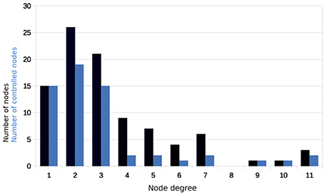
Figure 2. Number of nodes with a given degree (black) in a non-homogenous scale-free network with N = 100 nodes and normally distributed parameters and number of nodes of the given degree that need to be controlled (blue).

Note that in the notion of constructive control theory (see e.g., [19, 24]), the dynamics of the nodes that are not controlled establishes the zero dynamics (i.e., the dynamics resulting from the restriction that p_i = 0 for all i such that v_i ∈ V_c) and by construction this dynamics is asymptotically stable. Therefore, the zero dynamics correspond to a spreading process over a reduced network, from which the monitored (and thus controlled) nodes have been withdrawn, given that for p_i(t) ≡ 0 the node v_i does no longer interact with its neighbors.

3.2 Feedback Control Design

The question addressed in this section is how to design the feedback control for the nodes v_j ∈ V_C so that $\underset{t\to \infty }{lim}|p_j(t)-p_j^{*}|=0$. Up to this point, we have not considered the dependency of ζ(P, U) on U, given that U was considered as a set of constant parameters. This dependency will permit to explicitly determine a control law u_i(t) = β_i(t) that steers the nodes v_j ∈ V_C to their desired values $p_j^{*}=0$. With this idea, the following theorem is established

Theorem 1. Consider the dynamics given by (4) and consider the nodes that do not satisfy (13) as the set V_C of nodes to be controlled. Let V_M = V_C, that is, all controlled nodes are monitored. If the controls u_i(t) satisfy

$\begin{array}{cc}\begin{array}{c}0\le u_i(t)<{\stackrel{-}{\beta }}_i=\frac{{\tau }_i}{{\displaystyle {\sum }_{j=1}^N{r}_{ij}{a}_{ij}}},\end{array}& (15)\end{array}$

then (P^T, Q^T)^T = 0 is exponentially stable.

Proof. The Theorem can be easily proven as follows. Let ${\bar{\beta }}_i$ be given as in (15). It follows that

$\begin{array}{cc}0& \le u_i(t)<{\stackrel{-}{\beta }}_i,\\ \iff 0& \le u_i(t)r_{ij}{a}_{ij}<{\stackrel{-}{\beta }}_i{r}_{ij}{a}_{ij},\\ \iff 0& \le {\displaystyle \underset{j=1}{\overset{N}{{{\displaystyle \sum }}^{\text{}}}}}{u}_i(t)r_{ij}{a}_{ij}<{\displaystyle \underset{j=1}{\overset{N}{{{\displaystyle \sum }}^{\text{}}}}}{\stackrel{-}{\beta }}_i{r}_{ij}{a}_{ij}.\end{array}$

Given that for ${\beta }_i\le {\bar{\beta }}_i$ inequality (13) is satisfied, one obtains

$\begin{array}{r}0\le {\displaystyle \sum _{j=1}^N}{u}_i(t)r_{ij}{a}_{ij}<{\displaystyle \sum _{j=1}^N}{\bar{\beta }}_i{r}_{ij}{a}_{ij}<{\tau }_i,\end{array}$

or equivalently

$\begin{array}{r}{\displaystyle \sum _{j=1}^N}{u}_i(t)r_{ij}{a}_{ij}<{\tau }_i\end{array}$

implying that inequality (13) is satisfied. In consequence, the exponential stability of (P^T, Q^T)^T = 0 follows.     ▢

Note that following a similar reasoning, a control law can be established for the case that u_i(t) = r_ij(t). Nevertheless, this approach will not be explicitely elaborated at this place.

From Theorem 1, we have that in order to stabilize the extinction state for the dynamics (4) it is sufficient to design feedback controls u_i(t) for all nodes v_i ∈ V_C, which take values below the upper-bound ${\bar{\beta }}_i$ defined in (15). For example, a simple linear feedback control given by

$\begin{array}{cc}\begin{array}{r}{u}_i(t)={\beta }_i(t)=\gamma {\bar{\beta }}_i(1-p_i(t)),\gamma \in (0,1)\end{array}& (16)\end{array}$

does satisfy this condition. Note that the advantage of using a time varying control law β_i(t) consists in actively adapting the infection probability on the actual needs, i.e., the actual network state. In comparison with imposing a constant value for β_i this possibly enables to optimize the control effort over time, because according to (16) ${\beta }_i\to \gamma {\bar{\beta }}_i$ with p_i → 0. The performance using this simple output-feedback control is illustrated in the subsequent section.

3.3 Simulations

In order to verify our results, we perform several simulations of the dynamical system (4), for different initial conditions, with the following considerations

• We used a scale-free network of N = 10⁶ described by G(V, E), that incorporates preferential attachment according to Barabási and Albert [21]. We started with a small number m_o = 9 of vertices, linked randomly, and at every step we add a new node or vertex with m = 3 edges until we reach N = 10⁶. We emphasize that our results are independent of the network's topology.

• To facilitate our simulations, we consider that r_ij = r_ji.

• The constant values for the recovery probability μ_i, the probability of infection β_i, the internment probability τ_i, and the contact probability r_i were distributed uniformly over the nodes with values in the interval [0.2, 0.7].

• To show and corroborate our results, we calculated the average probability ρ(t) given by

$\begin{array}{cc}\begin{array}{r}\rho (t)=\frac{1}{N}{\displaystyle \sum _{i=1}^N}{p}_i(t).\end{array}& (17)\end{array}$

• The sets V_C and V_M are chosen according to Lemma 2 as the sets of nodes that do not satisfy (13). For the case considered here 424569 nodes out of N = 10⁶ (i.e., about 42.5%) have to monitored and controlled.

Simulation studies have been performed considering the following scenarios:

  I. Absence of control: All parameters of the system (4) have constant values which not necessarily satisfy condition (13).

 II. Zero dynamics: The output was constrained to Y(t) = 0 by setting β_j = 0 and p_j(0) = 0 for all v_j ∈ V_M = V_C.

III. Linear feedback control: The linear feedback control given by (16) has been implemented for all v_i ∈ V_M = V_C.

I. Absence of Control

In the absence of control the network reaches an endemic attractor state where about a 20% of the nodes are probably infected after about 20 time units as can be seen in Figure 3.

FIGURE 3

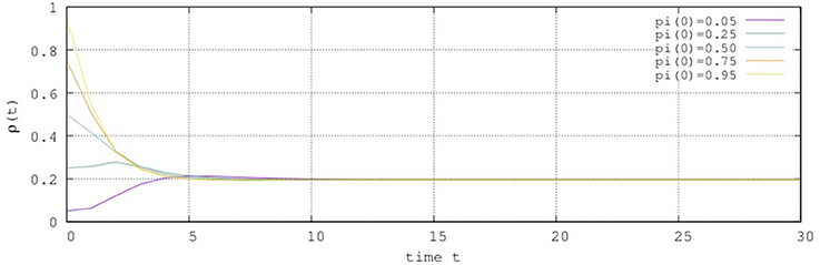
Figure 3. Behavior of ρ(t) for several initial conditions without control.

II. Zero Dynamics

To corroborate that the zero dynamics are exponentially stable, we set Y(t) = 0 for those nodes that do not satisfy (13). This is achieved by setting β_i = 0 for v_i ∈ V_M.

Figure 4 shows the behavior of the nodes associated with the zero dynamics. Note that the extinction state is reached after 18 time steps.

FIGURE 4

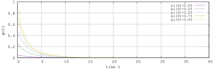
Figure 4. Behavior of the zero dynamics.

III. Linear Feedback Control

To show the performance of the proposed simple output-feedback control scheme (16), it has been implemented for all monitored and controlled nodes with the gain γ = 0.9 and the upper bound ${\bar{\beta }}_i$ calculated according to (15). This yields the output-feedback controller.

$\begin{array}{cc}\begin{array}{c}{\beta }_i(t)=\frac{\gamma {\tau }_i(1-p_i(t))}{{\displaystyle {\sum }_{j=1}^N{r}_j{a}_{ij}}},\text{\hspace{1em}for\hspace{1em}}\gamma =0.9\text{\hspace{1em}and\hspace{1em}}\forall v_i\in V_C=V_M.\end{array}& (18)\end{array}$

Note that the control (18), depends on the state of the node i given by p_i(t), and the properties of its neighbors given by ${\bar{\beta }}_i$. Figure 5 shows the result of the simulation with the applied control (18). As predicted in Theorem 1 the extinction state is a close-loop attractor, and is reached in about 40 time steps.

FIGURE 5

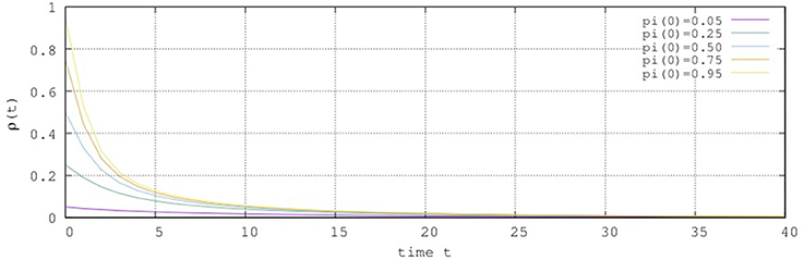
Figure 5. Closed-loop network behavior with the linear feedback control given by (18).

4. Discussions and Conclusions

The problem of deciding which nodes in a complex network with quarantine should be controlled and how to control them in order to achieve that in the closed-loop system the extinction state becomes a (global) attractor has been studied. Sufficient conditions for virus extinction have been derived using a constructive control approach by suitably identifying the zero dynamics according to a threshold condition for the stability of the extinction state. The associated node selection criterion does depend on the transmission probability between the nodes and their neighbors, the degree of each node and its probability to pass into quarantine. It has been shown that in spite of the strongly nonlinear dynamics of the spreading process the extinction state can be efficiently stabilized using a simple linear bounded output-feedback control if the nodes to be controlled are selected according to the proposed scheme. The performance and behavior of the spreading process without and with control has been illustrated for a scale-free network with N = 10⁶ nodes.

Author Contributions

All authors designed and did the research, in particular the stability analysis. LA-R and AS conceived and designed the control and the numerical experiments. LA-R performed the numerical experiments. All authors analyzed the data. LA-R and RB wrote the paper. All authors reviewed the manuscript. All authors have read and approved the final manuscript.

Funding

This work was partially sponsored by Rector office of UAM Cuajimalpa through Programa de Apoyo a Proyectos Interdisciplinarios.

Conflict of Interest Statement

The authors declare that the research was conducted in the absence of any commercial or financial relationships that could be construed as a potential conflict of interest.

References

1. Wang W, Tang M, Zhang HF, Gao H, Do Y, Liu ZH. Epidemic spreading on complex networks with general degree and weight distributions. Phys Rev E (2014) 90:042803. doi: 10.1103/PhysRevE.90.042803.

PubMed Abstract | CrossRef Full Text | Google Scholar

2. Leventhal GE, Hill AL, Nowak MA, Bonhoeffer S. Evolution and emergence of infectious diseases in theoretical and real-world networks. Nat Commun. (2015) 6:6101. doi: 10.1038/ncomms7101.

PubMed Abstract | CrossRef Full Text | Google Scholar

3. Tomovski I, Trpevski I, Kocarev L. Topology independent SIS process: An engineering viewpoint. Commun Nonlinear Sci Numer Simul. (2014) 19:627–37. doi: 10.1016/j.cnsns.2013.06.033.

CrossRef Full Text | Google Scholar

4. Wang Y, Chakrabarti D, Wang C, Faloutsos C. Epidemic spreading in real networks: an eigenvalue viewpoint. In: 22nd International Symposium on Reliable Distributed Systems, 2003. Florence. (2003). p. 23–5.

5. Chakrabarti D, Wang Y, Wang C, Leskovec J, Faloutsos C. Epidemic thresholds in real networks. ACM Trans Inf Syst Secur. (2008) 10:1–26. doi: 10.1145/1284680.1284681.

CrossRef Full Text | Google Scholar

6. Gómez S, Arenas A, Borge-Holthoefer J, Meloni S, Moreno Y. Discrete-time Markov chain approach to contact-based disease spreading in complex networks. Europhys Lett. (2010) 89:38009. doi: 10.1209/0295-5075/89/38009.

CrossRef Full Text | Google Scholar

7. Gómez S, Arenas A, Borge-Holthoefer J, Meloni S, Moreno Y. Probabilistic framework for epidemic spreading in complex networks. Int J Complex Syst Sci. (2011) 1:47–54. Available online at: http://www.ij-css.org/volume-01_01/ijcss01_01-047.pdf.

Google Scholar

8. Meloni S, Arenas A, Gomez S, Borge-Holthoefer J, Moreno Y. Modeling Epidemic Spreading in Complex Networks: Concurrency and Traffic. In: Thai MT, Pardalos PM, editors. Handbook of Optimization in Complex Networks. New York, NY: Springer. (2012). p. 435–62.

Google Scholar

9. Moreno Y, Nekovee M, Pacheco AF. Dynamics of rumor spreading in complex networks. Phys Rev E (2004) 69:066130. doi: 10.1103/PhysRevE.69.066130.

PubMed Abstract | CrossRef Full Text | Google Scholar

10. Borge-Holthoefer J, Moreno Y. Absence of influential spreaders in rumor dynamics. Phys Rev E (2012) 85:026116. doi: 10.1103/PhysRevE.85.026116.

PubMed Abstract | CrossRef Full Text | Google Scholar

11. Singh A, Singh YN. Rumor Spreading and Inoculation of Nodes in Complex Networks. In: Proceedings of the 21st International Conference on World Wide Web. WWW '12 Companion. New York, NY: ACM. (2012). p. 675–8.

Google Scholar

12. Xie M, Jia Z, Chen Y, Deng Q. Simulating the spreading of two competing public opinion information on complex network. Appl Math. (2012) 3:1074–8. doi: 10.4236/am.2012.39158.

CrossRef Full Text | Google Scholar

13. Mc'Kendrick AG. Applications of Mathematics to Medical Problems. Proc Edinburgh Math Soc. (1925) 44:98–130.

Google Scholar

14. Kermack WO, McKendrick AG. Contributions to the mathematical theory of epidemics. II. —The problem of endemicity. Proc R Soc Lond A Math Phys Eng Sci. (1932)138:55–83.

Google Scholar

15. Bernal Jaquez R, Schaum A, Alarcon L, Rodriguez C. Stability analysis for virus spreading in complex networks with quarantine. Publ Mat Uruguay (2013) 14:221–33. Available online at: http://pmu.uy/pmu14/pmu14.pdf.,

Google Scholar

16. Chimmalee B, Sawangtong W, Wiwatanapataphee B. The effects of community interactions and quarantine on a complex network. Cogent Math. (2016) 3:1249141. doi: 10.1080/23311835.2016.1249141.

CrossRef Full Text | Google Scholar

17. Alarcon-Ramos LA, Schaum A, Rodriguez Lucatero C, Bernal Jaquez R. Stability analysis for virus spreading in complex networks with quarantine and non-homogeneous transition rates. J Phys Conf Ser. (2014) 490:012011. doi: 10.1088/1742-6596/490/1/012011.

CrossRef Full Text | Google Scholar

18. Schaum A, Bernal Jaquez R. Estimating the state probability distribution for epidemic spreading in complex networks. Appl Math Comput. (2016) 29:197–206. doi: 10.1016/j.amc.2016.06.037.

CrossRef Full Text | Google Scholar

19. Monaco S, Normand-Cyrot D. Zero dynamics of sampled nonlinear systems. Syst Control Lett. (1988) 11:229–34.

Google Scholar

20. Isidori A. Nonlinear Control Systems. London: Springer (2000).

Google Scholar

21. Barabási AL, Albert R. Emergence of Scaling in Random Networks. Science (1999) 286:509–12.

PubMed Abstract | Google Scholar

22. Nowzari C, Preciado VM, Pappas GJ. Analysis and control of epidemics: a survey of spreading processes on complex networks. IEEE Control Syst. (2016) 36:26–46. doi: 10.1109/MCS.2015.2495000.

CrossRef Full Text | Google Scholar

23. Cullen CG. Matrices and Linear Transformations. New York, NY: Dover Publications. (1990).

Google Scholar

24. Byrnes CI, Lin W. Losslessness, feedback equivalence, and the global stabilization of discrete-time nonlinear systems. IEEE Trans Automatic Control (1994) 39:83–98.

Google Scholar