The Guedon-Vershynin Semi-definite Programming Approach to Low Dimensional Embedding for Unsupervised Clustering

1. Introduction

Low dimensional embedding is a key to many modern data analytics. Data are better understood after choosing the best coordinates, i.e., embedding, and extracting the main features. Based on a compressed description, the data can then be projected, visualized, or clustered more reliably and efficiently. The goal of the present paper is to present an efficient technique for joint embedding and clustering, based on pairwise affinity analysis and reliable convex optimization.

Combining the goals of reducing dimensionality and clustering in a principled manner is challenging and novel, but also draws on ideas from spectral clustering [1, 2], and Semi-Definite embedding, as in Linial et al. [3]. The main idea behind such methods, is to approximately preserve the pairwise distances in the dataset, with the goal of discovering, via an appropriate coordinate change, the correct parameterization of the potentially low dimensional non-linear manifold that essentially contains the data. An example of non-linear low dimensional embedding, such as Diffusion Maps, is shown in Figure 1.

FIGURE 1

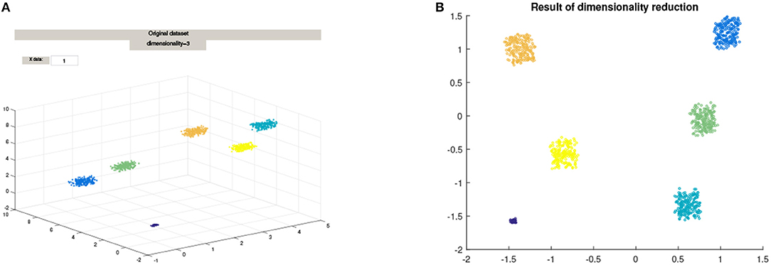
Figure 1. The mapping of a 3D cluster using Diffusion Maps from the Matlab package drtoolbox https://lvdmaaten.github.io/drtoolbox/. (A) Original 3D Cluster, (B) Mapped data using Diffusion Maps.

Apart from this previous works, standard clustering techniques usually start from already embedded data as obtained after e.g., PCA processing. Said otherwise embedding and clustering are often considered as completely separate tasks. Based on embedded data, mainstream clustering techniques are non-parametric (as K-means, K-means++, etc. [4, 5]) and model based clustering (as Mixture Models [6]). These approaches often rely on non-convex optimization such as Lloyd's algorithm and Expectation-Maximization [7, 8]. However, even careful implementation of these algorithms leads to some uncertainty as to whether one has finally obtained a relevant optimizer. In Mixture Model-based clustering, one also faces the issue of degeneracy [9]. As a result, a growing body of researched has emerged lately concerning the study of convex relaxation for the clustering problem [10, 11], etc. Other approaches such as ClusterPath [12] have also been proposed (see [13–15]) for interesting extensions. One drawback of theses approaches is the presence of many hyperparameters without robust rules to select them. The present work pursues this recent trend of promoting convex optimization-based clustering based on low rank cluster matrix estimation, as a way of ensuring that no spurious local optimizer is used in the process of clustering-based decision making in data analytic studies.

Our starting point in this attempt at finding appropriate embeddings for clustering is the method by Guedon and Vershynin [16], initially developed for community detection in the stochastic block model (SBM). In mathematical terms, the SBM considers a random graph based on a set of vertices partitioned into clusters and with random edges between vertices, all edges are independent and the probabilities of edges depend only on the cluster structure. The usual assumption made in the SBM is that the probabilities are larger within clusters than across clusters. The problem of recovering clusters from a random empirical adjacency matrix has been a topic of extensive research, triggered by the work of McSherry [17] and which quickly developed into a beautiful body of impressive results and achievements (see [18–22]). Guedon and Vershynin recently showed that the cluster matrix can be estimated via Semi-Definite Programming (SDP) with an explicit control of the error rate.

From a technical perspective, our contribution is three-fold.

• First, we generalize the Guedon/Vershynin approach in order to deal with the Gaussian Cluster Model (GCM) and show that the cluster matrix in the GCM can also be estimated by solving an SDP. For doing so, we use an affinity matrix as input that depends only on the pairwise distances between observations. Contrarily to the adjacency matrix arising in the SBM, our affinity matrix from the GCM has non independent entries, thus making the analysis non trivial.

• Our second contribution is to demonstrate in practice that the estimated cluster matrix yields a natural associated embedding. Indeed, quite similarly to spectral clustering, the eigenvectors of the estimated cluster matrix provide a meaningful embedding. Contrarily to standard embedding methods such as PCA, Laplacian eigenmaps, Maximum Variance Unfolding, t-SNE, etc., the embedding does not try to preserve pairwise distances but rather to estimate the cluster matrix. The intuition for using the cluster matrix is supported by Remark 1.6 in Guédon and Vershynin [16] which we now quote: It may be convenient to view the cluster matrix as the adjacency matrix of the cluster graph, in which all vertices within each community are connected and there are no connections across the communities. This way, the Semi-Definite program takes a sparse graph as an input, and it returns an estimate of the cluster graph as an output. The effect of the program is thus to “densify” the network inside the communities and “sparsify” it across the communities.

• Our third contribution is to propose a new scalable algorithm for solving the main Semi-Definite Programming problem at the heart of Guédon and Vershynin [16] and our approach to embedding and clustering. Our new method is based on a linearized version of the Alternating Direction Method of Multipliers (ADMM) together with a pragmatic implementation of the constraints, that allows us the avoid solving the original Semi-Definite Program via interior point methods.

The paper is organized as follows. The SDP approach for estimating the cluster matrix, the associated embedding and the main theoretical results are presented in section 2. The proofs are postponed to section 2 in the Appendix. The algorithmic considerations for the resolution of the SDP are discussed in the Supplementary Material, where an efficient algorithm is described as well as a practical method for selecting the unknown tuning parameter. Section 3 is devoted to the presentation of simulation results, demonstrating the potential of the proposed method. Some technical background on Gaussian concentration and Grothendieck inequality is provided in Appendices.

2. Main Results

2.1. Framework: The Gaussian Cluster Model

The mathematical framework is the following. We assume that we observe a data set x₁, …, x_n ∈ ℝ^d over a population of size n. The population is partitioned into K clusters ${{C}}_1,\dots ,{{C}}_K$ of size n₁, …, n_K, respectively, i.e., n = n₁+ ⋯ +n_K. We assume the standard Gaussian Cluster Model for the data: the observations x_i are independent with

$\begin{array}{ll}{x}_i~{N}({\mu }_k,{\Sigma }_k)\text{ if }i\in {{C}}_k& (1)\end{array}$

with ${\mu }_k\in {ℝ}^d$ the cluster mean and ${\Sigma }_k\in {ℝ}^{d\times d}$ the cluster covariance matrix. The Gaussian Mixture model specifies the additional information about the probabilities of belonging to each cluster and the Gaussian Cluster Model corresponds to conditioning the Gaussian Mixture Model on the values of the latent cluster indicator variables [6]¹.

The clustering problem aims at recovering the clusters ${{C}}_k$, 1 ≤ k ≤ K, based on the data x_i, 1 ≤ i ≤ n, only. For each i = 1, …, n, we will denote by k_i the index of the cluster to which i belongs. The notation i ~ j will mean that i and j belong to the same cluster. The cluster matrix $\bar{Z}$ is the n × n matrix defined by

$\begin{array}{ll}{\overline{Z}}_{i,j}=\{\begin{array}{cc}1& \text{if }i~j\hfill \\ 0& \text{otherwise}\hfill \end{array},1\le i,j\le n.& (2)\end{array}$

It determines entirely the clusters and, up to a reordering of the points, it is a block-diagonal matrix with a block of ones for each cluster.

Note that the Gaussian Cluster Model slightly differs from the usual Gaussian mixture model where the data set consists in independent observations from the Gaussian mixture $\sum _{k=1}^K{\pi }_k{N}({\mu }_k,{\Sigma }_k)$, with (π_k)_{1 ≤ k ≤ K} the mixture distribution. In the Gaussian mixture model, the cluster sizes (n₁, …, n_k) are random with multinomial distribution of size n and probability parameters (π₁, …, π_K).

2.2. Dimensionality Reduction

As proved in Bandeira et al. [23] the data can be projected onto a space of dimension log(K) while still preserving separation when the data are assumed to belong to separated ellipsoids. Therefore, we can consider in the rest of the paper that d is of the order of log(K). The results of our main theorem below will give the appropriate scaling of the parameters that will ensure the well separatedness of the data.

2.3. Embedding Associated With the Estimated Cluster Matrix

We will define in the next section an estimate $\hat{Z}$ of the cluster matrix $\bar{Z}$. We discuss now how a low dimensional embedding of the data set can be associated with the estimate $\hat{Z}$. The main idea is to use the fact that the cluster matrix $\bar{Z}$ defined by (2) has a very specific eigenstructure: denoting by ${{C}}_1$, …, ${{C}}_K$ the index set of each cluster and by $1_{{{C}}_k}\in {\left\{0,1\right\}}^n$ the indicator vector of cluster ${{C}}_k$, we have

$\begin{array}{l}\bar{Z}={\displaystyle \sum _{k=1}^K}{1}_{{{C}}_k}{1}_{{{C}}_k}^t\end{array}$

and we deduce that

• the rank of $\bar{Z}$ is K,

• the nonzero eigenvalues of $\bar{Z}$ are $\left|{{C}}_1\right|$, …, $\left|{{C}}_K\right|$ with associated eigenvectors $1_{{{C}}_1}/\sqrt{\left|{{C}}_1\right|},\dots ,1_{{{C}}_K}/\sqrt{\left|{{C}}_1\right|}$.

We assume in the sequel that the cluster sizes are all different so that all non-zero eigenvalues have multiplicity one. The clusters can hence be recovered from the eigenstructure of the matrix $\bar{Z}$: the label of the sample point x_i is the index of the only eigenvector whose i-th component is non zero. Indeed, all other eigenvectors associated with a non-zero eigenvalue have i-th component equal to zero.

The estimate $\hat{Z}$ of the matrix $\bar{Z}$ can be used in practice to embed the data into the space ℝ^K by associating each data point x_i to the vector consisting of the i-th coordinate of the K first eigenvectors of $\hat{Z}$. Given this embedding, if we can prove that $\hat{Z}$ accurately estimates the cluster matrix $\bar{Z}$, one can then apply any clustering method of choice to recover the clustering pattern of the original data. The next section gives a method for computing an estimator $\hat{Z}$ of $\bar{Z}$ using the SDP approach by Guedon and Vershynin.

2.4. Guedon and Vershynin's Semi-definite Program

We now turn to the estimation $\hat{Z}$ of the cluster matrix using Guedon and Vershynin's Semi-Definite Programming based approach. Whereas, Guédon and Vershynin [16] were interested in analyzing the Stochastic Block Model for community detection, we propose a study of the Gaussian Cluster Model and therefore prove that their approach has a great potential applicability in embedding of general data sets beyond the Stochastic Block Model setting.

Based on the data set x₁, …, x_n, we construct the affinity matrix A by

$\begin{array}{ll}A=(f(||x_i-x_j|{|}_2){)}_{1\le i,j\le n}& (3)\end{array}$

where ||·||₂ denotes the Euclidean norm on ℝ^d and f :[0, +∞) → [0, 1] a non-increasing affinity function. A popular choice is the Gaussian affinity

$\begin{array}{ll}f(h)=e^{-{(h/h_0)}^2},h\ge 0,& (4)\end{array}$

with h₀ > 0, and other possibilities are

$\begin{array}{c}f(h)=e^{-{(h/h_0)}^a},f(h)={\left(1+\left(h/h_0\right)\right)}^{-a},\\ f(h)={\left(1+e^{h/h_0}\right)}^{-a}\cdots \end{array}$

Before stating the Semi-Definite Program, we introduce some matrix notations. The usual scalar product between matrices A, B ∈ ℝ^n×n is denoted by $\langle A,B\rangle =\sum _{1\le i,j\le n}{A}_{ij}{B}_{ij}$. The notations $1_n\in {ℝ}^n$ and $1_{n\times n}\in {ℝ}^{n\times n}$ stand for the vector and matrices with all entries equal to 1. For a symmetric matrix Z ∈ ℝ^n×n, the notation Z ⪰ 0 means that Z the quadratic form associated to Z is non-negative while the notation Z ≥ 0 means that all the entries of Z are non-negative.

With these notations, we define $\hat{Z}$ as a solution of the Semi-Definite Program

$\begin{array}{ll}\text{maximize}\langle A,Z\rangle \text{subject to }Z\in {{M}}_{opt}& (5)\end{array}$

with ${{M}}_{opt}$ the set of symmetric matrices Z ∈ ℝ^n×n such that

$\begin{array}{ll}\{\begin{array}{l}Z⪰0\hfill \\ Z\ge 0\hfill \\ \text{diag}(Z)=1_n\hfill \\ \langle Z,1_{n\times n}\rangle ={\text{λ}}_0\hfill \end{array}.& (6)\end{array}$

Here λ₀ ∈ ℕ is the number of non-zero edges in the true cluster matrix and Guedon and Vershynin state in Guedon and Vershynin [16] that it can be estimated empirically. For further reference, note that a semi-definite positive matrix Z with non-negative entries and unit diagonal must have all entries in [0, 1], so that ${{M}}_{opt}\subset {\left[0,1\right]}^{n\times n}$.

The heuristic justifying that $\hat{Z}$ can be seen as an estimate of the cluster matrix $\bar{Z}$ is the following Lemma.

Lemma 2.1. Consider the expected affinity matrix

$\begin{array}{ll}Ā=(\text{E}f(||x_i-x_j|{|}_2){)}_{1\le i,j\le n}.& (7)\end{array}$

and assume

$\begin{array}{ll}p={\displaystyle \underset{i~j}{inf}}{Ā}_{i,j}>q={\displaystyle \underset{i\nsim j}{sup}}{Ā}_{i,j}.& (8)\end{array}$

Then, the cluster matrix $\bar{Z}$ defined by Equation (2) is the unique solution of

$\begin{array}{ll}maximize\langle Ā,Z\rangle subjecttoZ\in {{M}}_{opt}& (9)\end{array}$

with ${\lambda }_0=\sum _{k=1}^K{n}_k^2$.

The intuition behind condition (8) is that the average distance (or more precisely the average affinity) between two points within a same cluster is smaller than the average distance between two points from different clusters. This corresponds to the intuitive notion of clusters. Note that a similar condition appears in Guédon and Vershynin [16]. In the case of the Gaussian affinity function (4), we provide in section 2.6 explicit formulas for the expected affinity matrix that can be used to check condition (8).

The SDP (5) appears as an approximation of the SDP (9) since the affinity matrix A can be seen as a noisy observation of the unobserved matrix Ā. Concentration arguments together with Grothendieck theorem allow to prove that A ≈ Ā in the sense of the ℓ^∞/ℓ¹-norm (see Proposition 2.4 below). In turn, this implies $\hat{Z}\approx \bar{Z}$ in the sense of ℓ¹-norm in ℝⁿ² (see Theorem 2.2 below) so that the SDP program (5) provides a good approximation $\hat{Z}$ of the cluster matrix $\bar{Z}$. Note that in practice, λ₀ is unknown and must be estimated (see comment in section 5.1.5).

Proof of Lemma 2.1: This corresponds to Lemma 7.1 in Guédon and Vershynin [16]. □

2.5. Theoretical Error Bounds

Our main result is a non asymptotic upper bound for the probability that $\hat{Z}$ differs from $\bar{Z}$ in ℓ¹-distance, that is an upper bound for

$||\hat{Z}-\bar{Z}|{|}_1={\displaystyle \sum _{1\le i,j\le n}}|{\hat{Z}}_{i,j}-{\bar{Z}}_{i,j}|.$

Theorem 2.2. Consider the Gaussian Cluster Model (1) and assume that the affinity function f is ℓ-Lipschitz and that condition (8) is satisfied. Let

$\begin{array}{l}{t}_0=8\sqrt{2log2}{K}_G\sigma \ell /(p-q)\end{array}$

where K_G ≤ 1.8 denotes the Grothendieck constant and ${\sigma }^2=\frac{1}{n}\sum _{k=1}^K{n}_k\rho ({\Sigma }_k)$ with ρ(Σ_k) the largest eigenvalue of the covariance matrix Σ_k.

Then, for all t > t₀,

$\begin{array}{ll}\text{P}\left(\Vert \hat{Z}-\bar{Z}{\Vert }_1>n^{2}t\right)\le 2exp\left(-{\left(\frac{t-t_0}{c}\right)}^{2}n\right),& (10)\end{array}$

$\begin{array}{ll}c=\frac{16\sqrt{2}{K}_G\ell \sigma }{p-q}.& (11)\end{array}$

Moreover, there exists a subset τ ⊂ {1, …, n} with $\left|\tau \right|\ge \frac{n}{2}$ such that all t > t₀,

$\begin{array}{ll}\text{P}\left(\left|\right|{\left(\hat{Z}-\bar{Z}\right)}_{\tau \times \tau }|{|}_1>nt\right)\le 2exp\left(-{\left(\frac{t-t_0}{c}\right)}^{2}n\right).& (12)\end{array}$

Proof: See section A.1 in the Appendix. □

Theorem 2.2 has a simple consequence in terms of estimation error rate. After computing $\hat{Z}$, it is natural to estimate the cluster graph $\bar{Z}$ by a random graph obtained by putting an edge between vertices i and j if ${\hat{Z}}_{i,j}>1/2$ and no edge otherwise. Then the proportion π_n of errors in the prediction of the n(n − 1)/2 edges is given by

$\begin{array}{l}{\pi }_n:=\frac{2}{n(n-1)}{\displaystyle \sum _{1\le i<j\le n}}|1_{\{{\hat{Z}}_{ij}>1/2\}}-{\bar{Z}}_{ij}|\\ \le \frac{2}{n(n-1)}{\displaystyle \sum _{1\le i<j\le n}}2|{\hat{Z}}_{ij}-{\bar{Z}}_{ij}|\hfill \\ =\frac{2}{n(n-1)}\left|\right|\hat{Z}-\bar{Z}|{|}_1.\hfill \end{array}$

The following corollary provides a simple bound for the asymptotic error.

Corollary 2.3. We have almost surely

${\displaystyle \underset{n\to \infty }{lim\; sup}}{n}^{-2}\Vert \hat{Z}-\bar{Z}{\Vert }_1\le t_0=\frac{8\sqrt{2log2}{K}_G\sigma \ell }{p-q}.$

In the case when the cluster means are pairwise different and fixed while the cluster variances converge to 0, i.e., σ → 0, it is easily seen that the right hand side of the above inequality behaves as O(σ) so that the error rate converges to 0. This reflects the fact that when all clusters concentrates around their means, clustering becomes trivial.

While our proof of Theorem 2.2 follows the ideas from Guédon and Vershynin [16], we need to introduce new tools to justify the approximation A ≈ Ā in ℓ^∞/ℓ¹-norm. Indeed, unlike in the stochastic block model, the entries of the affinity matrix (3) are not independent. We use Gaussian concentration measure arguments to obtain the following concentration inequality. The ℓ^∞/ℓ¹ norm of a matrix M ∈ ℝ^n×n is defined by

$\begin{array}{ll}\left|\right|M|{|}_{\infty \to 1}={\displaystyle \underset{\left|\right|u|{|}_{\infty }\le 1}{sup}}|\left|Mu\right|{|}_1={\displaystyle \underset{u,v\in {\left\{-1,1\right\}}^n}{max}}{\displaystyle \sum _{i,j=1}^n}{u}_i{v}_j{M}_{i,j}.& (13)\end{array}$

Proposition 2.4. Consider the Gaussian cluster model (1) and assume the affinity function f is ℓ-Lipschitz. Then, for any $t>2\sqrt{2log2}\ell \sigma$,

$\begin{array}{l}P(\left|\right|A-Ā|{|}_{\infty \to 1}>t{n}^2)\\ \le 2exp\left(-\frac{{\left(t-2\sqrt{2log2}\ell \sigma \right)}^2}{32{\ell }^2{\sigma }^2}n\right).& (14)\end{array}$

Proof: See section A.2 in the Appendix. □

Theorem 2.2 assumes that λ₀ is known. It is worth noting that λ₀ corresponds to the number of edges in the cluster graph and that we can derive from the proof of Theorem 2.2 how the algorithm behaves when the cluster sizes are unknown, i.e., when the unknown parameter λ₀ is replaced with a different value λ. The intuition is given in Remark 1.6 in Guédon and Vershynin [16]: if λ < λ₀, the solution $\hat{Z}$ will estimate a certain subgraph of the cluster graph with at most λ₀ − λ missing edges; if λ > λ₀, the solution $\hat{Z}$ will estimate a certain supergraph of the cluster graph with at most λ − λ₀ extra-edges.

2.6. Explicit Formula for Ā

In order to check condition (8), explicit formulas for the mean affinity matrix are useful. The next proposition solves the case of the Gaussian affinity function.

Proposition 2.5. Assume that A is built using the Gaussian affinity function (4).

• Let i and j be in the same cluster ${{C}}_k$. Then,

${Ā}_{i,j}={\displaystyle \prod _{l=1}^d}{\left(1+4{({\sigma }_{k,l}/h_0)}^2\right)}^{-1/2}$

with ${({\sigma }_{k,l}^2)}_{1\le l\le d}$ the eigenvalues of Σ_k.

• Let i and j be in different clusters ${{C}}_k$ and ${{C}}_{k^{\prime }}$. Then,

$\begin{array}{l}{\overline{A}}_{i,j}={\displaystyle \prod _{l=1}^d\exp }\left(-\frac{{\langle {\mu }_k-{\mu }_{k^{\prime }},v_{k,k^{\prime },l}\rangle }^2}{h_0^2+2{\sigma }_{k,k^{\prime },l}^2}\right)\\ {\left(1+2{({\sigma }_{k,k^{\prime },l}/h_0)}^2\right)}^{-1/2}\end{array}$

with ${({\sigma }_{k,k^{\prime },l}^2)}_{1\le l\le d}$ and ${(v_{k,k^{\prime },l})}_{1\le l\le d}$ respectively the eigenvalues and eigenvectors of ${\Sigma }_k+{\Sigma }_{k^{\prime }}$.

Proof: See section A.3 in the Appendix. □

As an interesting consequence of Proposition 2.5, when the variance matrices from the Gaussian Cluster Model (1) are all equal and isotropic, that is ${\Sigma }_k={\sigma }^2\text{Id}$ for all k = 1, …, K with σ² > 0, then the constants p and q from Equation (8) are given by

$p={\left(1+4{\sigma }^2/h_0^2\right)}^{-d/2}$

and

$q={\left(1+4{\sigma }^2/h_0^2\right)}^{-d/2}$

$\times {\displaystyle \underset{1\le k\ne k^{\prime }\le K}{min}}exp\{-||{\mu }_{k^{\prime }}-{\mu }_k|{|}^2/(h_0^2+4{\sigma }^2)\}.$

Condition (8) is therefore satisfied (whatever the choice of h₀ > 0) as soon as the cluster means (_{μk)1 ≤ k ≤ K} are pairwise distinct which is a minimal identifiability condition. But of course the difference p − q is an increasing function of the noise σ² and the bounds in Theorem 2.2 become looser for larger noise.

3. Simulation Results

In all the experiments, the parameter h₀ in (4) was chosen as

$h_0=.5*max{(\text{diag}(X^t*X))}^{1/2}.$

The hyper-parameter λ was chosen so as to minimize the mean squared error between the estimated cluster matrix and the empirical affinity matrix.

3.1. Computing the Actual Clustering From the Eigenvector Coordinates

As for spectral clustering, the components of the most significant eigenvectors, i.e., the eigenvectors associated with the largest eigenvalues, are the coordinates of the embedded data. Given these embedded data, as advised in Vu [24], the actual clustering can be computed using a minimum spanning tree method and removing the largest edges.

3.2. Comparison With Standard Embeddings on a 3D Cluster Example

Simulations have been conducted to assess the quality of the proposed embedding. In this subsection, we used the Matlab package drtoolbox² proposed by Laurens Van Maatten on a sample drawn from a 10 dimensional Gaussian Mixture Model with four components and equal proportions. In Figure 2, we show the original affinity matrix together with the estimated cluster matrix. In Figure 3, we compare the affinity matrix of data with the affinity matrix of the mapped data using various embeddings proposed in the drtoolbox package. This toy experiment shows that the embedding described in this paper can cluster as the same time as it embeds into a small dimensional subspace. This is not very surprising since our embedding is tailored for the joint clustering-dimensionality reduction purpose whereas most of the known existing embedding methods aren't. Given the fact that clustered data are ubiquitous in real world data analysis due to the omnipresence of stratified populations, taking the clustering purpose into account might be a considerable advantage.

FIGURE 2

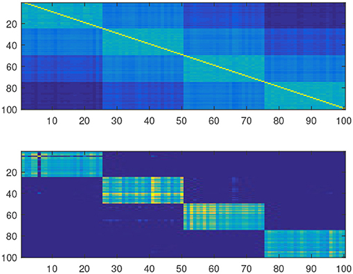
Figure 2. Original affinity matrix vs. Guedon Vershynin Cluster matrix.

FIGURE 3

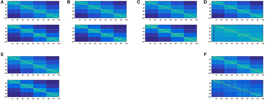
Figure 3. The affinity matrix obtained after embedding using different methods from the Matlab package drtoolbox https://lvdmaaten.github.io/drtoolbox/. (A) Original affinity matrix vs. affinity matrix after PCA embedding. (B) Original affinity matrix vs. affinity matrix after MDS embedding. (C) Original affinity matrix vs. affinity matrix after Factor Analysis embedding. (D) Original affinity matrix vs. affinity matrix after t-SNE embedding. (E) Original affinity matrix vs. affinity matrix after Sammon embedding. (F) Original affinity matrix vs. affinity matrix after LLE embedding.

3.3. Monte Carlo Experiments

In this section, we present some simulation experiments assessing the performance of the Guedon-Vershynin embedding for Gaussian Cluster Models.

3.3.1. Setup

Our experiments were performed on problems of successive sample size 100, 200, …, 1,000 and number of clusters equal to 2, 5, and 10. The dimension of the Gaussian Mixture Model was set to 100. For each experiment, we performed 100 Monte Carlo repeats. All the results in this section show the average over the Monte Carlo experiments. Our Gaussian Cluster Model was built as follows: for a model with K clusters, we set the kth component of each center to 10/3, 20/3, …, 50/3 for each cluster k = 1, …, K. Then, the data are obtained by adding a unit variance i.i.d. Gaussian vector to the center of the cluster it belongs to. All clusters were taken to have equal size.

3.3.2. Selection of λ

The value of λ was selected so as to minimize the Frobenius distance between Ẑ and A. Model based selection rules will be discussed in a follow up paper.

3.3.3. Results

Figures 4, 5 show the estimation error $\parallel \bar{Z}-Ẑ{\parallel }_1$ between the true and the estimated cluster matrix. These results illustrate Theorem 2.2 as they show that the error grows as a function of sample size. Moreover, the growth is quadratic as predicted by the theory of section 2, and more precisely Equation (10).

FIGURE 4

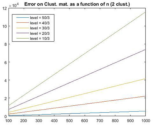
Figure 4. Estimation error $\parallel \bar{Z}-Ẑ{\parallel }_1$.

FIGURE 5

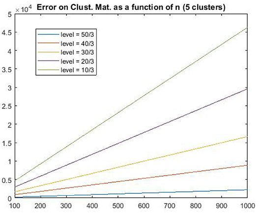
Figure 5. Estimation error $\parallel \bar{Z}-Ẑ{\parallel }_1$.

4. Conclusions

The goal of the present paper was to propose an analysis of Guedon and Vershynin's Semi-Definite Programming approach to the estimation of the cluster matrix and show how this matrix can be used to produce an embedding for preconditioning standard clustering procedures. The procedure is suitable for very high dimensional data because it is based on pairwise distances only. Moreover, increasing the dimension will improve the robustness of the procedure when the Law of Large Numbers will apply along dimensions, hence forcing the affinity matrix to converge to a deterministic limit and thus making the estimator less sensitive to its low dimensional fluctuations.

Another feature of the method is that it may apply to a large number of mixtures type, even when the component's densities are not log-concave, as do a lot of embeddings as applied to data concentrated on complicated manifolds. Further studies will be performed in this exciting direction.

Future work is also needed for proving that the proposed embedding is provably efficient when combined with various clustering techniques. One of the main reason why this should be a difficult problem is that the approximation bound proved in the present paper is not so easy to leverage for controlling the perturbation of the eigenspaces of Z. More precise use of the inherent randomness of the perturbation, in the spirit of Vu [24], might be necessary in order to go a little further in this direction.

Author Contributions

SC and CD contributed the theoretical analysis and the proofs. SC and AF contributed the code and simulation experiments for the initial version of this work. SC contributed the new algorithm and the corresponding simulation experiments.

Conflict of Interest Statement

AF was employed by company DigitalSurf.

The remaining authors declare that the research was conducted in the absence of any commercial or financial relationships that could be construed as a potential conflict of interest.

Acknowledgments

The results presented in this paper have appeared previously as Chapter 3 of the third author's Ph.D. thesis [25].

Supplementary Material

The Supplementary Material for this article can be found online at: https://www.frontiersin.org/articles/10.3389/fams.2019.00041/full#supplementary-material

Footnotes

1. ^Extending our study to the setting of Gaussian Mixture Models using the relationship with the Gaussian Cluster Model based on this conditioning is a somewhat tedious but not difficult task.

2. ^https://lvdmaaten.github.io/drtoolbox/

References

1. Von Luxburg U. A tutorial on spectral clustering. Stat Comput. (2007) 17:395–416.

Google Scholar

2. Bandeira AS. Ten Lectures and Forty-Two Open Problems in the Mathematics of Data Science (2015).

Google Scholar

3. Linial N, London E, Rabinovich Y. The geometry of graphs and some of its algorithmic applications. Combinatorica. (1995) 15:215–45.

Google Scholar

4. Jain AK. Data clustering: 50 years beyond k-means. Pattern Recogn Lett. (2010) 31:651–66. doi: 10.1016/j.patrec.2009.09.011

CrossRef Full Text | Google Scholar

5. Friedman J, Hastie T, Tibshirani R. The Elements of Statistical Learning, Vol. 1. Springer Series in Statistics. New York, NY: Springer Verlag (2001).

Google Scholar

6. McLachlan G, Peel D. Finite Mixture Models. John Wiley & Sons (2004).

PubMed Abstract | Google Scholar

7. Dempster AP, Laird NM, Rubin DB. Maximum likelihood from incomplete data via the EM algorithm. J R Stat Soc B. (1977) 39:1–38.

Google Scholar

8. Chrétien S, Hero AO. On EM algorithms and their proximal generalizations. ESAIM Probabil Stat. (2008) 12:308–26.

Google Scholar

9. Biernacki C, Chrétien S. (2003). Degeneracy in the maximum likelihood estimation of univariate gaussian mixtures with EM. Stat Probabil Lett. 61:373–82. doi: 10.1016/S0167-7152(02)00396-6

CrossRef Full Text | Google Scholar

10. Awasthi P, Bandeira AS, Charikar M, Krishnaswamy R, Villar S, Ward R. Relax, no need to round: integrality of clustering formulations. In: Proceedings of the 2015 Conference on Innovations in Theoretical Computer Science (ACM) (2015). p. 191–200.

Google Scholar

11. Mixon DG, Villar S, Ward R. Clustering subgaussian mixtures by semidefinite programming. arXiv preprint arXiv:1602.06612 (2016).

Google Scholar

12. Hocking TD, Joulin A, Bach F, Vert JP. Clusterpath an algorithm for clustering using convex fusion penalties. In: 28th International Conference on Machine Learning (2011). p. 1.

Google Scholar

13. Tan KM, Witten D. Statistical properties of convex clustering. Electron J Stat. (2015) 9:2324–47.

PubMed Abstract | Google Scholar

14. Radchenko P, Mukherjee G. Consistent clustering using an ℓ_1 fusion penalty. arXiv preprint arXiv:1412.0753 (2014).

Google Scholar

15. Wang B, Zhang Y, Sun W, Fang Y. Sparse convex clustering. arXiv preprint arXiv:1601.04586 (2016).

Google Scholar

16. Guédon O, Vershynin R. Community detection in sparse networks via grothendieck's inequality. Probabil Theory Relat Fields. (2015) 165:1025–49.

Google Scholar

17. McSherry F. Spectral partitioning of random graphs. In: Proceedings 2001 IEEE International Conference on Cluster Computing (IEEE) (2001). p. 529–37.

Google Scholar

18. Abbe E, Bandeira AS, Hall G. Exact recovery in the stochastic block model. arXiv preprint arXiv:1405.3267 (2014).

Google Scholar

19. Heimlicher S, Lelarge M, Massoulié L. Community detection in the labelled stochastic block model. arXiv preprint arXiv:1209.2910 (2012).

Google Scholar

20. Mossel E, Neeman J, Sly A. Stochastic block models and reconstruction. arXiv preprint arXiv:1202.1499 (2012).

Google Scholar

21. Mossel E, Neeman J, Sly A. Reconstruction and estimation in the planted partition model. Probabil Theory Relat Fields. (2015) 162:431–61. doi: 10.1007/s00440-014-0576-6

CrossRef Full Text | Google Scholar

22. Mossel E, Neeman J, Sly A. A proof of the block model threshold conjecture. Combinatorica (2018.) 38:665–708.

Google Scholar

23. Bandeira AS, Mixon DG, Recht B. Compressive classification and the rare eclipse problem. In: Compressed Sensing and Its Applications. Springer (2017). p. 197–220.

Google Scholar

24. Vu V. Singular vectors under random perturbation. Random Struct Algorthm. (2011) 39:526–38.

Google Scholar

25. Faivre A. Analyse d'image hyperspectrale (PhD thesis). Université de Bourgogne, Franche-Comté, France (2018).

Google Scholar

26. Tropp JA. Column subset selection, matrix factorization, and eigenvalue optimization. In: Proceedings of the Twentieth Annual ACM-SIAM Symposium on Discrete Algorithms (Society for Industrial and Applied Mathematics) (2009). 978p. –86.

Google Scholar

27. Wang H, Banerjee A. Bregman alternating direction method of multipliers. In: Advances in Neural Information Processing Systems (2014). p. 2816–24.

Google Scholar

28. Boucheron S, Lugosi G, Massart P. Concentration Inequalities: A Nonasymptotic Theory of Independence. Oxford: Oxford University Press (2013).

Google Scholar