Deductron—A Recurrent Neural Network

1. Introduction

Recurrent Neural Networks (RNN) have gained significant attention in recent years due to their success in many areas, including speech recognition and image-to-text conversion and Optical Character Recognition (OCR) [1, 2]. These are systems which respond to sequential inputs such as time series. With skillfull implementation, they have the ability to react to the stimuli in real time which is at the root of their applications to building intelligent systems. The classes of RNN which memorize and forget a certain amount of information are especially interesting.

Yet, it is hard to find in literature examples of data which can be easily understood, and which demonstrably require remembering and forgetting information to operate correctly. In this paper we will provide such an example of data, define the related machine learning problem and solve it using typical machine learning tools. Our analysis will be rigorous whenever possible, reflecting our mathematical and computer science point of view. Thus, we will constantly pivot between three subjects (math, computer science, and connectionist artificial intelligence) hopefully providing an insightful study, which can be continued in various directions by the reader. We also included a number of exercises varying in the degree of difficulty which should make reading more fun.

Several review-type survey articles on RNN exist, providing a comprehensive discussion of various RNN architectures and survey of results and techniques [3–5]. We do not attempt to provide such a survey, but we rather focus on some key aspects of the theory which we feel are not covered by existing work. Specifically, in the current paper we are interested in explaining the need for long-term memory, in addition to short-term memory. In the last 20 years LSTM (Long-Short Memory) RNNs have been applied to a variety of problems with artificial intelligence flavor, in particular, speech-to-text conversion and optical character recognition [6, 7]. We find that typical examples used to illustrate LSTM are too complex to understand how the network performs its task. In particular:

(1) Why is there a need for long and short term memory in specific problems?

(2) How does one discover good neural network architectures? Are there general approaches?

(3) Are neural networks interpretable?

Let us further define the problem of interpretability of a neural net model. This problem has become central in current research [8]. The essence of a neural model is captured in a (typically) large set of parameters, the weights, which is often beyond the human ability of comprehension of data. In particular, the significance to the application domain is often a mystery, and the user must treat the model as a black box. On the other hand, conventional, imperative computer programs can be understood, and are often constructed by the domain experts, thus capturing the essential knowledge of the domain as a set of rules. Given a neural net model, can we develop the underlying rule system?

In order to address these questions, we construct:

(1) a simple, synthetic dataset which captures the essential features of the OCR problem for cursive scripts, such as Arabic;

(2) a simple, yet powerful RNN architecture suitable for solving the OCR problem;

(3) a process of discovery of RNN architectures, in which the essential step is a transition between a “conventional” algorithm and a “connectionist” solution in the form of RNN; it is important that the process can be carried out in both directions:

(a) the process provides a method to define RNN architectures, starting with a conventional (imperative, rule based) program to solve simple instances of the application domain problem;

(b) the process provides an interpretation of an RNN, in the form of a computer program that could be written and understood by a human programmer; the construction of the program must be automated.

While the above outline will be addressed in significant detail, several other directions will be deferred to future papers. In particular, the current paper will not contain large-scale “real life” applications of the deductron architecture. However, significant evidence has accumulated already, demonstrating that the deductron may be used in place of well-known RNN architectures, LSTM and GRU, with similar, and sometimes better outcomes. In particular, the deductron architecture is not a toy architecture and it can be used in real applications. Examples are described in section 11. Notably, a detailed example in which we use deductron as an LSTM replacement is presented in section 11.2.

2. The W-Language and Long-Term Memory

In order to have a suitable example of data, we constructed a simple (artificial) writing system (we will call it the W-language, or “wave language”), encoding characters 'X' and 'O' as their upper halves, i.e., ∨ and ∧ (this is possible due to reflectional symmetry of 'X' and 'O' and no other two Latin characters would do). The characters can be connected, as in some languages. Thus, 'XOOXXO' is encoded in our alphabet as '∨∧∧∨∨∧'. Hence, the written text looks like a sequence of waves, with one restriction: a wave that starts at the bottom (top), must end at the bottom (top).

Let us explain the fact that decoding sequences of characters requires long-term memory. It is clear that seeing a sequence fragment '|∧∧∧∧∧|' of any length does not allow us to decode the sequence as '…XXX…' or '…OOO …' due to inherent ambiguity. Thus, it is necessary to remember the beginning of the “wave” (bottom or top) to resolve this ambiguity. Hence the need for memory; in fact, we need to remember what was written an arbitrarily long time ago in order to determine whether a given sequence should be decoded as a sequence of 'X' or as a sequence of 'O'.

Having invented our (artificial) writing system, we construct an RNN (in some ways similar to LSTM) capable of decoding sequences like the examples provided above, with 100% accuracy in the absence of errors. In the presence of errors, the accuracy should gracefully drop off, demonstrating robustness; this will not be pursued in the current paper.

What we will focus on is a construction of the RNN network in an unusual, and hopefully enlightening way. Rather than proposing a network architecture in a “blue skies research” fashion (or looking at prior work), we wrote a conventional program which decodes the sequences as the example above, operating on a binary image representation, with vertical resolution of three pixels. Subsequently, we re-interpreted the program as a neural network, and thus obtained a neural network “by inspection” (the only non-trivial example of this sort we are aware of). We then generalized this neural network to discover a new RNN architecture whose instance is our handcrafted RNN. It turns out to be a three-layer network, where the middle layer is capable of performing simple logical inferences; thus the name deductron will be used for our newly discovered architecture.

The next stage of our study is to pursue machine learning, using the new RNN architecture. We considered two methods of machine learning:

(1) Simulated annealing;

(2) Stochastic Gradient Descent (SGD).

In particular, we developed a training algorithm for the new architecture, by minimizing a standard cost function (also called the loss function in the machine learning community) with simulated annealing. The training algorithm was demonstrated to find a set of weights and biases of the neural network which yields a decoder capable of solving the decoding problem for the W-language. In some runs, the decoder is logically equivalent to the manually constructed decoder. Thus, we proved that our architecture can be trained to write programs functionally equivalent to hand-coded programs written by a human. It is possible to learn a decoding algorithm from a single sample of length 30 (encoding the string 'XOOXXO').

We also applied a different method of training the deductron called back-propagation through time (BPTT) and known to succeed in training other RNNs. This, and other back-propagation based algorithms require computing gradients of complicated functions, necessitating application of the Chain Rule over complex dependency graphs. Modern tools perform the gradient calculation automatically. One such tool is Tensorflow [9]. We implemented machine learning using Tensorflow and some programming in Python. We took advantage of the SGD implementation in Tensorflow. In particular, we used the Adam optimizer [10]. Using standard steps, we demonstrated that the decoder for the W-language can be constructed by learning from a small sample of valid sequences (of length ≈ 500).

Both simulated annealing and BPTT methods worked with relative ease when applied to our problem of decoding the W-language.

3. The W-language and Writing System Formalism

In the current paper we study a toy example of a system for sending messages like:

…XOOXXO…

The message is thus expressed as a string in alphabet consisting of letters 'X' and 'O'. However, we assume that the message is transcribed by a human or a human-like system, by writing it on paper, and scanning it to a digital image, e.g., like in Figure 1.

FIGURE 1

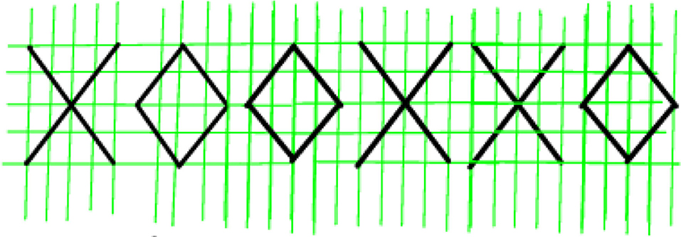
Figure 1. Handwritten sample representing string 'XOOXXO'.

Letters 'X' and 'O' were chosen because they are symmetric with respect to reflections along the horizontal axis. We assume that the receiver of the message sees only the upper half of the message, which could look like Figure 2. Thus, our effective alphabet is

${A}=\left\{\vee ,\wedge \right\}.$

However, when rendering the messages in this alphabet, we may connect the consecutive characters, as in various script-based languages, i.e., we write in cursive. The message is also subject to errors of various kinds, resulting in something like Figure 3. More severe errors could be, for instance, random bit flips, i.e., the input message could be subjected to the binary symmetric channel [11].

FIGURE 2

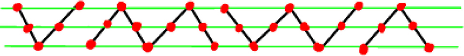
Figure 2. The top portion of the handwritten sample representing string 'XOOXXO'.

FIGURE 3

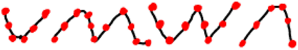
Figure 3. The top portion of the handwritten sample representing string 'XOOXXO', with some errors.

For the purpose of constructing a minimalistic example still possessing the features of the motivating example, we think of digitized representations of the messages, which are five pixels tall. Thus, the “top” of the message is only three pixels tall, and it consists of a sequence of vectors representing the columns of the image. Let us introduce the vectors appearing in the messages, first using standard mathematical notations, and their pictorial equivalents:

These are the vectors which may occur if we are precisely observing the rules of calligraphy of our messages, as illustrated by Figure 1. We adopt the following convention:

Convention 1 (Increasing direction of index). The following rules will be adhered to throughout the paper:

(1) In the mathematical notation, components of (column) vectors are numbered by an index that increases downwards (the usual “textbook” convention);

(2) In the corresponding pictorial representation the index increases upwards.

Based on the experiences of the readers of the drafts of this paper, it is expected that the reader will need to refer to the above formal convention when certain index calculations become confusing.

Our sample message 'XOOXXO' is thus represented by the sequence of vectors:

$\begin{array}{l}0,{\text{e}}_3,{\text{e}}_2,{\text{e}}_1,{\text{e}}_2,{\text{e}}_3,{\text{e}}_1,{\text{e}}_2,{\text{e}}_3,{\text{e}}_2,{\text{e}}_1,{\text{e}}_2,{\text{e}}_3,{\text{e}}_2,{\text{e}}_1,{\text{e}}_3,{\text{e}}_2,{\text{e}}_1,{\text{e}}_2,\\ {\text{e}}_3,{\text{e}}_2,{\text{e}}_1,{\text{e}}_2,{\text{e}}_3,{\text{e}}_1,{\text{e}}_2,{\text{e}}_3,{\text{e}}_2,{\text{e}}_1,0.\end{array}$

We can also represent the message pictorially as a 3 × 30 image, i.e., a matrix of bits, as in Figure 4A, obtained by concatenation of pictorial representations of the vectors representing the message. In Figure 4B we represent the image as raw data (a 2D matrix of bits).

FIGURE 4

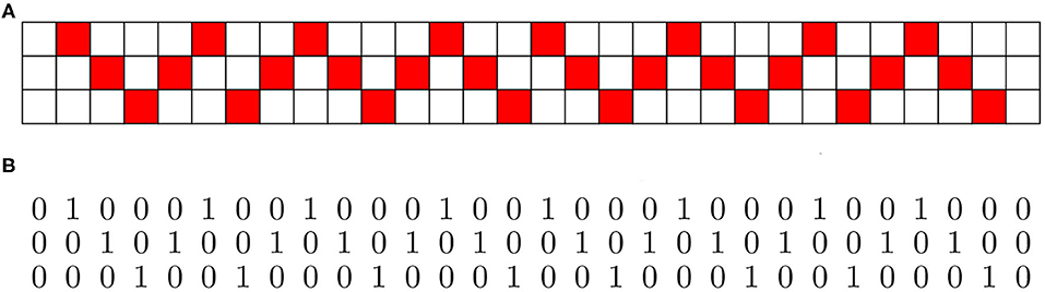
Figure 4. Two equivalent representations of a W-language message, one of which could be produced on an ordinary typewriter. (A) Binary image of the message ‘XOOXXO’. (B) Binary image of the message ‘XOOXXO’ as raw bits; a typewriter equivalent of the above.

We could consider “errors” obtained by inserting extra 0 vectors between e₁ and e₃ signaling a long break between symbols 'X' and 'O'. We could repeat some vectors. Generally, the image should consist of a number of “waves” and “breaks”. We note that the “wave” portion of the pattern may be arbitrarily long. However, a picture like Figure 5 cannot be interpreted as a long sequence '…XXXX…' or '…OOOO…'. We must go back to the last “break” (one of the transitions 0 → e₁, 0 → e₃, e₂ → e₁, e₂ → e₃) which begins a run of 'O' or 'X'. Thus decoding an image like Figure 2 is very similar to decoding a sequence encoded using Run Length Encoding (RLE), in which we code runs of characters 'X' and 'O'. The transition tells us whether we are starting an 'X' (∗ → e₃, where ∗ denotes 0 or e₂) or 'O' (∗ → e₁).

FIGURE 5

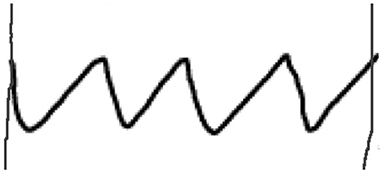
Figure 5. A wave.

The image consists of a certain number of complete waves possibly separated with breaks. A properly constructed complete wave begins and ends in the same vector, either e₁ or e₃. It can be divided into rising and falling spans. For example, a rising span would be a sequence e₁, e₂, e₂, e₃, e₃. That is, the non-zero coordinate of the vector moves upwards. A break is simply a run of 0 vectors. Such a run must be preceded and followed by e₁ or e₃. Since the rising and falling spans are of arbitrary length, we must remember whether we are rising or falling, to validate the sequence, and to prevent spans like e₃, e₂, e₂, …, e₂, e₃ which should not occur in a valid sequence. A complete wave starting with e₃ must begin with a falling span, and alternate rising and falling spans afterwards, finally terminating with a rising span. In order to decode a wave correctly as a sequence of 'X' or 'O', we must remember whether we are currently rising or falling.

In short, we have to remember two things:

(1) Are we within 'X' or 'O'?

(2) Are we rising or falling?

There is some freedom in choosing the moment when to emit a character 'X' or 'O'. We could do it as soon as we begin a rising or falling span terminating in the vector which started the wave. Or we can wait for completion of the span, e.g., when a rising span ends and a falling span begins, or has a jump e₃ → e₁ or e₃ → 0 (jump e₃ → e₂ would be an error).

There is a simple graphical model (a topological Markov chain, also called a subshift of finite type) which generates all error-free sequences which can be decoded in Figure 6. As we can see, the states of the Markov chain correspond to the vectors 0, e₁, e₂, and e₃, except that vector e₂ has two corresponding states: ${\text{e}}_2^{\pm }$. The state ${\text{e}}_2^{+}$ (${\text{e}}_2^{-})$ can only be entered when we encounter vector e₂ on a rising (falling) span. Thus, the state ${\text{e}}_2^{\pm }$ is a state that “remembers” whether it is on a rising or falling span. The total number of states is thus 5.

FIGURE 6

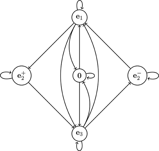
Figure 6. The topological Markov chain which can be used to generate training data for our network. A valid transition sequence should start and end on one of the nodes: e₁, e₃, or 0. Thus, it cannot start or end at ${\text{e}}_2^{\pm }$.

In computer science and computer engineering the more common term is finite state machine (FSM) or finite state automaton. This is essentially a Topological Markov Chain with distinguished initial and final states. Our Topological Markov Chain generates complete expressions of the W-language iff they start at 0, e₁, or e₃. Thus, initial and final states are these three states.

Exercise 1 (Regular W-language generation). Draw a diagram, analogous to Figure 6 which describes only those sequences in which the rising and falling spans never stall, thus no frame repeats. We can call the resulting language a strict W-language. Assume that there are no breaks between symbols, i.e., connecting two consecutive 'X' or 'O' is mandatory. ♠

Exercise 2 (Higher resolution W-languages). Our W-language uses vertical resolution of 3 pixels. Define language W_k in which symbols are k pixels high. Consider the strict variant, also. ♠

4. A Conventional W-Language Decoding Algorithm

Our next goal is to devise a simple algorithm which will correctly decode the sequences encoded in the W-language. We emphasize that the algorithm is “conventional” rather than “connectionist,” although the lines between these two approaches to programming will be (deliberately) blurred in the following sections. In order to correctly decode an image like in Figure 4A processing it sequentially, by column, from left to right, we need to detect and memorize the events associated with starting a new character. The detection is possible by looking at a “sliding window” of 2 consecutive column vectors. In Table 1 we listed patterns of vectors in both columns that let us determine whether we are starting a new character. Let

$X=\left[\begin{array}{cc}{x}_{1,1}& x_{1,2}\\ x_{2,1}& x_{2,2}\\ x_{3,1}& x_{3,2}\end{array}\right]$

be the sliding window. We note that the matrix X is “upside down” relative to the image in Figure 4A, due to conflicting conventions. Matrices, like X and their mapping to computer memory, are written starting with the first row at the top, and the image in Figure 4A has the first row of pixels at the bottom. The mapping of elements of matrix X to the pixels is made explicit in Figure 7.

TABLE 1

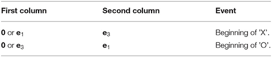
Table 1. Recognizing character boundaries.

FIGURE 7

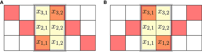
Figure 7. Sliding windows at the boundary of two characters. (A) Window at the end of 'O' and start of 'X'. (B) Window at the end of 'X' and start of 'O'.

The beginning of 'X' is thus detected by the logic statement:

$x_{2,1}=0\wedge x_{3,1}=0\wedge x_{3,2}=1$

Similarly, the beginning of 'O' is detected by the logic statement:

$x_{2,1}=0\wedge x_{1,1}=0\wedge x_{1,2}=1$

These conditions can be expressed using auxiliary variables:

$\begin{array}{l}{y}_1=\neg x_{2,1}\wedge \neg x_{3,1}\wedge x_{3,2}\\ y_2=\neg x_{2,1}\wedge \neg x_{1,1}\wedge x_{1,2}\end{array}$

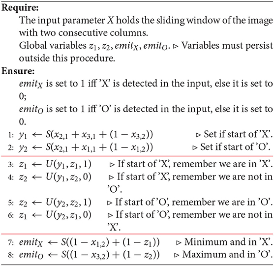
The event can be recorded and memorized by setting variables z₁ and z₂ which indicate whether we are at the beginning of 'X' and 'O', respectively. By convention, the meaning of the values of z₁ and z₂ is just given in Table 2. We also will use the vector z = (z₁, z₂). Knowing z₁ and z₂ allows us to emit 'X' or 'O' when we encounter the extreme values e₁ and e₃. We observe that 'X' is emitted upon encountering a minimum in signal, i.e., value e₁, while 'O' is emitted upon encountering a maximum, i.e., e₃. Table 3 summarizes the actions which may result in emitting a symbol. The action on every sliding window may result in setting the value of z₁ or z₂ and/or emitting a symbol. Whether the symbol is emitted or not will be signaled by setting a variable emit_X or emit_O, respectively. In the algorithm, emit_X and emit_O are global variables; their values persist outside the program. The program tells the caller that an 'X' or 'O' was seen. The caller calls the program on all frames (sliding windows) in succession, from left to right.

TABLE 2

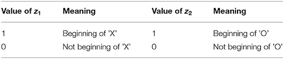
Table 2. The meaning of z₁ and z₂.

TABLE 3

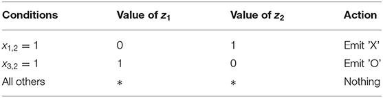
Table 3. Character emission rules.

ALGORITHM 1

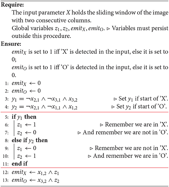
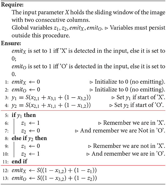
Algorithm 1. A basic, handcrafted algorithm for decoding an image representing a sequence of 'X' and 'O'.

It is clear that an algorithm which correctly performs decoding should look like Algorithm 1. We divided the algorithm into three sections, with horizontal lines. These sections nearly exactly correspond to the three layers of the neural network (deductron), which will be constructed from this program. Although we designed our algorithm to use a sliding window, this is not necessary (Hint: You can buffer your data from within your algorithm, using persistent, i.e., global variables).

Exercise 3 (Elimination of sliding window). Design an algorithm similar to Algorithm 1 which takes a single column (frame) of the image as input. ♠

Exercise 4 (Pixel at a time). Design a similar algorithm to Algorithm 1 which takes a single pixel as input, assuming vertical progressive scan: pixels are read from bottom-to-top, and then left-to-right. ♠

Exercise 5 (Counting algorithms). Count the number of distinct algorithms similar to Algorithm 1. That is, count the algorithms which:

(1) operate on a sliding window with 6 pixels;

(2) use two 1-bit memory cells;

(3) produce two 1-bit outputs.

Clearly, one of them is our algorithm. ♠

Exercise 6 (The precise topological Markov chain). Note that the transition graph in Figure 6 allows for generation of partial characters 'X' and 'O'. For example, the sequence:

$0,{\text{e}}_1,{\text{e}}_2^{+},{\text{e}}_3,0$

would result in emitting an 'O' by our program, but the 'O' would never be completed. Prove that the transition diagram in Figure 8 enforces completion of characters. In fact, prove that this topological Markov chain is 100% compatible with Algorithm 1. What is the role of superscripts “f” and “s”? ♠

FIGURE 8

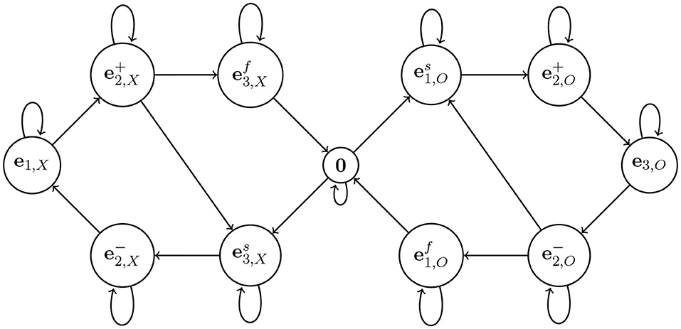
Figure 8. An improved topological Markov chain. The idea is to have essentially two copies of the diagram in Figure 6, the left part for 'X' and the right part for 'O'. Also, some states are split to enforce completion of characters (the states with superscript “f” are “final” in generating each character).

Exercise 7 (Deductron and Chaotic Dynamics). In this exercise we develop what can be considered a custom pseudorandom number generator, which generates valid sequences in the W-language. It mimics the operation of a linear congruential random number generator (e.g., [12], Chapter 3). This exercise requires some familiarity with Dynamical Systems, for example, in the scope of Chapter 6 of [13]. Figure 9 we have an example of a simple chaotic dynamical system: a piecewise linear mapping of an interval f:[0, 11) → [0, 11). This mapping is piecewise expanding, i.e., |f′(x)| > 1 except for the discontinuities. In fact, f′(x) ∈ {2, 4}. The intervals [k, k + 1), k = 0, 1, …, 8 are in 1:1 correspondence with the states of the Markov chain in Figure 8. This allows us to generate valid expressions of the W-language by using the dynamics of f. We simply choose a random initial condition x₀ ∈ [0, 9) and create a trajectory by successive applications of f:

$x_{n+1}=f(x_n).$

Let k_n be a sequence of numbers such that x_n ∈ [k_n, k_n + 1) for n = 0, 1, …. Let s_n be the corresponding sequence of states labeling the intervals, in the set

$\left\{{\text{e}}_{3,X}^s,{\text{e}}_{2,X}^{-},{\text{e}}_{1,X},{\text{e}}_{2,X}^{+},{\text{e}}_{1,X},{\text{e}}_{3,X}^f,0,{\text{e}}_{1,O}^s,{\text{e}}_{2,O}^{+},{\text{e}}_{3,O},{\text{e}}_{2,X}^{-},{\text{e}}_{1,X}^f\right\}.$

The idea is the second subscript ('X' or 'O') keeps track of which symbol we are in the middle of. The superscript ± on ${\text{e}}_{2,X}^{\pm }$ and ${\text{e}}_{2,O}^{\pm }$ keeps track of whether we are rising or falling, as before. The superscripts 's' (for 'start') and 'f' (for 'finish') indicate whether we are starting or finishing the corresponding character. Thus, ${\text{e}}_{3,X}^s$ means we are starting an 'X', and ${\text{e}}_{3,X}^f$ means we are finishing an 'X'. The difference is that a finished character must be followed by a blank or the other character, and must not continue the same character. Prove that s₀, s₁, …, s_n, … is a valid sentence the W-language. Conversely, show that for every such sentence there is an initial condition x₀ ∈ [0, 11) reproducing this sentence. Moreover, for infinite sentences x₀ is unique.♠

FIGURE 9

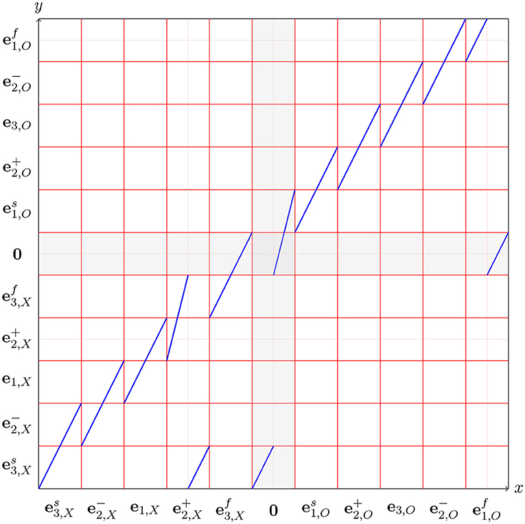
Figure 9. A piecewise linear mapping f:[0, 11) → [0, 11), in which every piece has slope 2 or 4. The intervals [k, k + 1) are labeled with the states of the topological Markov chain in Figure 8.

5. Converting a Conventional Program to a Neural Net

Our ultimate goal is to construct a neural network which will decode the class of valid inputs. A neural network does not evaluate logical expressions and does not have the control structure of conventional programs. Instead, it performs certain arithmetical calculations and it outputs results based on hard or soft thresholding.

The next step toward a neural network consists in rewriting our program so that it uses arithmetic instead of logic, and has no control structures, such as “if” statements. We replace logical variables with real variables, but initially we restrict their values to 0 and 1 only. It is important that the logical operations (“and,” “or,” and negation) are performed as arithmetic on real values.

The conditions in Algorithm 1 can be expressed arithmetically (as every prepositional calculus formula can). We introduce the variables:

$\begin{array}{l}{y}_1=S(x_{2,1}+x_{3,1}+(1-x_{3,2}))\\ y_2=S(x_{2,1}+x_{1,1}+(1-x_{1,2}))\end{array}$

where S is a function on integers defined by

$\begin{array}{ll}S(a)=\{\begin{array}{cc}1& a\le 0,\\ 0& a\ge 1.\end{array}& (1)\end{array}$

S plays the role of an activation function, in the language of neural computing. Variables y₁ and y₂ are conceptually related to perceptrons, or, in language closer to statistics, they are binary linear classifiers. We note that this function allows an easy test of whether a number of variables are 0. Variables u₁, u₂, …, u_r with values in the set {0, 1} are all zero iff

$S\left({\displaystyle \sum _{j=1}^r}{u}_j\right)=1.$

We obtain Algorithm 2. The final adjustment to the algorithm is made in Algorithm 2 in which we replace all conditionals with arithmetic. This results in Algorithm 3.

ALGORITHM 2

Algorithm 2. A version of the basic, handcrafted algorithm for decoding an image representing a sequence of 'X' and 'O' in which logical operations were replaced with arithmetic.

ALGORITHM 3

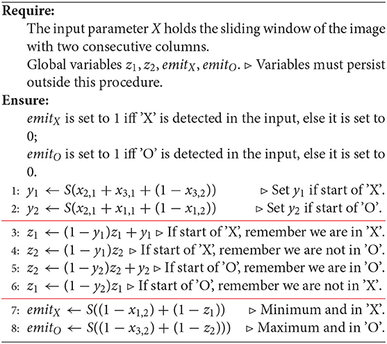
Algorithm 3. A version of the basic, handcrafted algorithm for decoding an image representing a sequence of 'X' and 'O' in which all conditionals were converted to arithmetic. We can view this code as an algorithm calculating activations and outputs of a neural network with several types of neurons.

Upon close inspection, we can regard the algorithm as an implementation of a neural network with several types of neurons (gates).

(1) Perceptron-type, with formula

$y_i=S\left({\displaystyle \sum _j}{w}_{ij}{x}_j+b_i\right).$

(2) “Forget and replace” gate:

$z^{\prime }=U(y,z,z^{\prime })$

where

$U(y,z,z^{\prime })=\{\begin{array}{cc}{z}^{\prime }& y=1,\\ z& y=0.\end{array}$

Or arithmetically,

$U(y,z,z^{\prime })=(1-y)·z+y·z^{\prime }.$

This kind of gate provides a basic memory mechanism, where z is preserved if y = 0, or replaced with z′ if y = 1.

Using the newly introduced U-gate we rewrite our main algorithm as Algorithm 4.

ALGORITHM 4

Algorithm 4. A version of the basic, handcrafted algorithm for decoding an image representing a sequence of 'X' and 'O'. Explicit gates are used to underscore the neural network format.

6. An Analysis of the U-gate and a New V-gate

The U-gate implements in essence the modus ponens inference rule of prepositional logic:

$\begin{array}{l}p,p\to q\Rightarrow q.\end{array}$

Indeed, p represents the replace port of a U-gate. The assignment q ← U(p, q, 1) is equivalent to p → q in the following sense: the boolean variable q represents a bit stored in memory. If p is true, q is asserted, i.e., set to true, so that the logical expression p → q is true (has value 1). Similarly, the assignment q ← U(p, q, 0) is equivalent to p → ¬q, i.e., q is set to 0, so that p → ¬q is true. Thus, if q is set to 1, the fact q is retracted, and the fact ¬q is asserted. This semantics is similar to the semantics of the Prolog system without variables, where we have a number of facts, such as “q” or “¬q”, in the Prolog database. Upon execution, facts can be asserted or retracted from the database.

Thus, the inference layer consists of:

(1) a number of variables q₁, q₂, …, q_n with some values of the variables set to either 0 or 1. Some of the variables may not be initialized, i.e., hold an undefined value;

(2) a number of assignments q_j ← U(p_k, q_j, r_j) where r_j = 0 or r_j = 1, where the order of the assignments matters; the order may only be changed if the new order will always result in the same values for all variables after all assignments are processed; some assignments can be performed in parallel, if they operate on disjoint sets of variables q_j, so that the order of processing of the groups does not affect the result; the same variable q_j may be updated many times by different U-gates. That is, later gates in the order may overwrite the result of the former gates.

In the interaction between the variables q_j and r_j, which are the result of binary classification, and variables p_j, which represent the memory of the system, it proves beneficial to assume that p_j is controlled by only two variables, and the final value of p_j after processing one input is represented by another kind of gate, the V-gate, which combines the action of two U-gates.

The V-gate operates according to the formula:

$V(z,u,v)=(1-u)(1-v)z+u$

where z stands for a memory variable (replacing p in our naming convention used in the context of the U-gate). A different (equivalent) formula for V-gate is:

$V(z,u,v)=\{\begin{array}{l}z\text{ when }u=v=0\text{,}\\ u\text{ when }v=1\text{.}\end{array}$

Equivalently, in logic terms we have several wff's of propositional calculus which represent V:

$\begin{array}{l}V(z,u,v)=u\vee (\neg v\wedge z)\\ =u\vee \neg (v\vee \neg z)\\ =(z\to v)\to u.\end{array}$

The action of the variables u and v on z is expressed as the assignment:

$z\leftarrow V(z,u,v).$

We will adopt the following approach: every memorized variable z will be controlled by exactly two variables: u and v. The rationale is that there are only two possible values of z. Therefore, if multiple assignments are made to z, the final result can be equivalently computed by combining those multiple assignments. This is equivalent to performing conjunction of multiple controlling variables u and v. The conjunction can be done by adding more variables to the first perceptron layer (adding together activations is equivalent to the end operation). Hence, only one V-gate is necessary to handle the change of the value of a memory variable z. The use of gate V is illustrated by the following example:

Example 1 (W-language decoding). In this example, we consider Algorithm 3. Instead of using a U gate, we can use the V-gate. Indeed, the assignments

z₁ ← (1 − y₁)z₁ + y₁      ⊳ If start of 'X', remember we are in 'X'.

z₂ ← (1 − y₁)z₂      ⊳ If start of 'X', remember we are not in 'O'.

z₂ ← (1 − y₂)z₂ + y₂      ⊳ If start of 'O', remember we are in 'O'.

z₁ ← (1 − y₂)z₁      ⊳ If start of 'O', remember we are not in 'X'.

can be rewritten as:

z₁ ← (1 − y₁)(1 − y₂)z₁ + y₁

z₂ ← (1 − y₁)(1 − y₂)z₂ + y₂

i.e.,

z₁ ← V(z₁, y₁, y₂)

z₂ ← V(z₂, y₂, y₁)

Hence, y₁ and y₂ are controlling both z₁ and z₂. ♣

Algorithm 5 is a modification of the previous algorithms which does not use the input values in the output layer. This is achieved by using the input layer (binary classification of the inputs) to memorize some input values in the memories (variables z_j). This technique demonstrates that the output layer of a deductron performing only binary classification of the memories (variables z_j) is sufficiently general without explicitly utilizing input values.

ALGORITHM 5

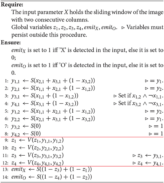
Algorithm 5. The final three-layer deductron architecture utilizing 4 memory cells.

Let us finish this section with a mathematical result proven by our approach:

Theorem 1 (On deductron decoding of W-language). There exists a deductron with 4 memory cells which correctly decodes every valid expression of the W-language.

Proof. As we constructed the deductron by writing an equivalent pseudocode, we prove first that one of the presentations of the algorithm, e.g., Algorithm 1, decodes the W-language correctly. The proof is not difficult and it uses the formal definition, which is essentially Figure 6. The tools to do so, such as loop invariants, are standard in computer science. Another part of the proof is to show that the neural network yields the same decoding as the pseudocode, even if the real arithmetic is only approximate. The details are left to the reader.     □

Exercise 8 (3 memory cells suffice for W-language). Prove that there exists a deductron with 3 memory cells correctly decoding W-language. For instance, write a different conventional program which uses fewer variables, and convert it to a 3-cell deductron. ♠

Exercise 9 (2 memory cells insufficient for W-language). Prove that there is no deductron with 2 memory cells, which correctly decodes every expression of the W-language. ♠

Exercise 10 (2 memory cells suffice for strict W-language). Prove that there is a deductron with 2 cells, which correctly decodes every expression of the strict W-language. ♠

Exercise 11 (1 memory cell insufficient for strict W-language). Prove that there is no deductron with 1 memory cell, which correctly decodes every expression of the strict W-language. ♠

As a hint for the previous exercises, we suggest studying Shannon information theory. In particular, the Channel Coding Theorem gives us the necessary tools to obtain a bound on the number of memory cells. Essentially, the memory is the “bottleneck” for passing information between inputs and outputs. Of course, information is measured in bits and it does not need to be a whole number.

ALGORITHM 6

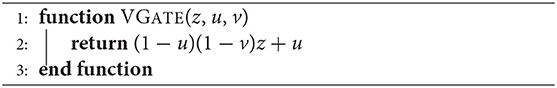
Algorithm 6. A V-gate simulator. We note that V(z, u, v) = (1 − u)(1 − v)z + u. If z, u and v are vectors of equal length, all operations are performed elementwise.

Upon considering the structure of the neural network based on perceptron layers and the new V-gate seen in Figure 10, we can see that our network is a 3-layer network. The first and third layer are perceptron layers, thus performing binary linear classification. We will call the first perceptron layer the input layer and the third layer the output layer.

FIGURE 10

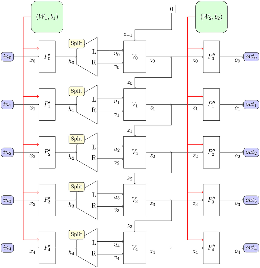
Figure 10. The deductron neural network architecture suitable for BPTT. The deductron is replicated as many times as there are inputs (frames). The perceptron $P_j^{\prime }$ classifies the input vectors x_j, which are subsequently demuxed and fed into the V-gates V_j, along with the content of the memory z_j−1, and the output is sent to memory z_j. The output of z_j is fed into the output classifier $P_j^{″}$. and output vector o_j is produced. Perceptrons $P_j^{\prime }$ share common weights W₁ and biases b₁. Perceptrons $P_j^{″}$ share common weights W₂ and biases b₂.

The middle layer is a new layer containing V-gates. We will call this layer the inference layer, as indeed it is capable of formal deduction of predicate calculus. We now proceed to justify this statement.

The general architecture based on V gate is quite simple and it comprises:

(1) The input perceptron layer, producing n_hidden = 2n_memory paired values u_i and v_i, i = 1, 2, …, n_memory, where n_memory is the number of memory cells;

(2) The inference (memory) layer, consisting of n_memory memory cells whose values persist until modified by the action of the V-gates; the update rule for the memory cells is

$z_i\leftarrow V(z_i,u_i,v_i)$

for i = 1, 2, …, n_memory.

(3) The output perceptron layer, which is a binary classifier working on the memory cells.

The semantics of the neural network can be described by the simulation algorithm, Algorithm 7 which expresses the process of creation of outputs as standard pseudocode.

ALGORITHM 7

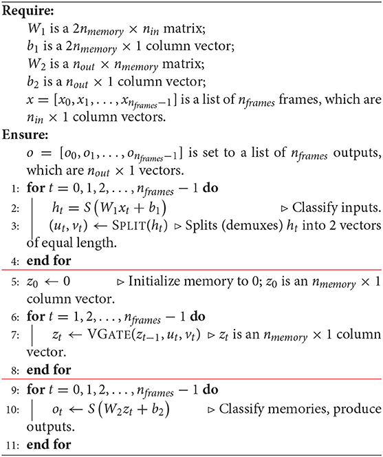
Algorithm 7. A simulator for our 3-layer deductron network. Note: The activation function S operates on vectors elementwise.

Figure 10 is a rudimentary systems diagram and can be considered a different presentation of Algorithm 7, focused on movement of data in the algorithm. This is especially useful in building circuits for training deductrons. As for other neural networks, there are two computational complexity estimates of importance:

(1) The computational cost of applying the network to data (easy);

(2) The computational cost of training the network (hard).

Let us estimate the computational cost of applying the network to data, i.e., performing Algorithm 7.

Theorem 2 (On time complexity of deductron). Let the input of the deductron in Figure 10 consist of frames of size n_in and let n_frames be the number of frames. Let n_memory ≥ 1 be the number of memory cells. Let n_out be the size of the output frame. Then the time complexity of producing the output (according to Algorithm 7) is:

$\begin{array}{ll}O\left((n_{in}+n_{out})·n_{memory}·n_{frames}\right).& (2)\end{array}$

Proof. As usual, we assume constant time complexity of individual arithmetical operations, assignments, and evaluating functions S and V. The dominant contributions come from the two matrix multiplications, with cost O(n_in · n_memory) and O(n_memory · n_out), repeating for every frame. The number of evaluations of S and V is O(n_memory · n_frames). We may assume that all sizes are ≥1, which leads to the total (2).     □

7. Interpretability of the Weights as Logic Formulas

Obviously, it would be desirable if the weights found by a computer could be interpreted by a human as “reasonable steps” to perform the task. In most cases, formulas obtained by training a neural network cannot be interpreted in this manner. For once, the quantity of information reflected in the weights may be too large for such an interpretation. Below we express some thoughts particular to training the deductron using simulated annealing on the W-language.

In Table 4 we listed some lines of the output produced by a simulated annealing run, and in Table 5 we see the weights found in this run. When a bias equals the number of −1's in the corresponding row of the matrix, it is apparent that that row of weights corresponds to a formula of logic (conjunction of inputs or their negations). However, in some runs (due to randomization), we obtain weights which do not correspond to logic formulas. Clearly, some of the rows of the weight W₁ and biases b₁ do not have this property.

TABLE 4

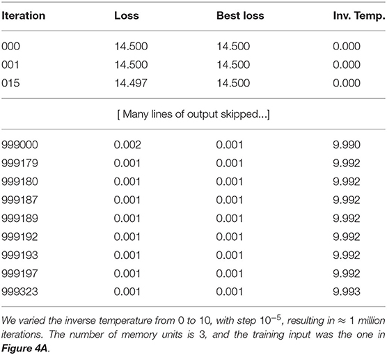
Table 4. A sample simulated annealing run.

TABLE 5

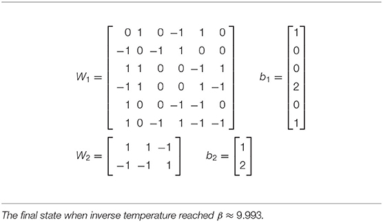
Table 5. Optimal weights learned by simulated annealing run in Table 4.

Example 2 (Weights and biases obfuscating a simple logic formula). Let us consider weights and biases obtained in one numerical experiment:

(1) A row of weights [1, 1, 0, −1, 0, 1];

(2) Bias 3.

Since two of the weights are 1, with a single weight of −1, the activation computed using it is at least 2. The activation is in the region where S yields a near-zero. Hence, the hidden unit constantly yields 0 (false), thus is equivalent to a simple, trivial propositional logic formula (false). ♣

Example 3 (Weights and biases without an equivalent conjunction). Let us consider weights and biases obtained in one numerical experiment:

(1) A row of weights [0, 1, −1, 1, 1, −1];

(2) Bias 1.

Thus the activation is x₁ − x₂ + x₃ + x₄ − x₅ + 1. Assuming that x_j ∈ {0, 1}, there is no conjunction of x_j, ¬x_j, or true, j = 0, 1, …, 5, equivalent to this arithmetic formula (the reader is welcome to prove this).

Nevertheless, there is a complex logical formula which is a disjunction of conjunctions, true only for solutions of this equation. This demonstrates that the logical formulas expressing the arithmetic equation can be more complex than just conjunctions, as in our manually constructed program. It is clear that any arithmetic linear equation or inequality over rational numbers can be expressed as a single logical formula in disjunctive normal form (disjunction of conjunctions). ♣

Exercise 12 (Disjunction of conjunctions for a linear inequality). Consider the linear inequality

$x_1-x_2+x_3+x_4-x_5+1>0$

over the domain x_j ∈ {0, 1}, j = 0, 1, …, 5. Construct an equivalent logical formula, which is a conjunction of disjunctions of some of the statements x_j = 0 or x_j = 1. ♠

Algorithm 7 defines a class of programs parameterized by weights and biases. The program expressed by Algorithm 3 can be obtained by choosing the entries of the weight matrices $W_1=\left[w_{ij}^{(1)}\right]$ and $W_2=\left[w_{ij}^{(2)}\right]$ and the bias vectors $b_1=\left[b_i^{(1)}\right]$ and $b_2=\left[b_i^{(2)}\right]$ so that:

(1) Each weight $w_{ij}^{(k)}$, k = 1, 2, is chosen to be ±1 or 0;

(2) Each entry $b_j^{(k)}$ is chosen to be the count of −1's in the i-th row of the matrix W_k.

With these choices, the matrix product expresses the value of a formula of propositional calculus. This is implied by the following:

Lemma 1 (Arithmetic vs. logic). Let W, b, x, and y be real matrices such that:

(1) W = [w_ij], 1 ≤ i ≤ m, 1 ≤ j ≤ n, w_ij∈{−1, 0, 1};

(2) x = [x_j], 1 ≤ j ≤ n, x_j∈{0, 1};

(3) b = [b_i], 1 ≤ i ≤ m, where b_i is the count of −1 amongst w_i1, w_i2, …, w_in;

(4) y = Wx.

Then

$y_i={\displaystyle \sum _{j=1}^n}{w}_{ij}{x}_j={\displaystyle \underset{j=1}{\overset{n}{\wedge }}}{x}_{ij},1\le i\le m$

where

$\begin{array}{l}{x}_{ij}=\{\begin{array}{ll}{x}_j& w_{ij}=1,\\ \neg x_j& w_{ij}=-1,\\ \mathrm{true}& w_{ij}=0.\end{array}\end{array}$

Proof. Left to the reader.     □

Exercise 13 (A formula for biases). Prove that under the assumptions of Lemma 1.

$b_i={\displaystyle \sum _{j=1}^n}g(w_{ij})$

where

$g(w)=\frac{w(w-1)}{2}=\genfrac{}{}{0.0pt}{}{w}{2}.$

♠

8. Machine Learning

It remains to demonstrate that the neural network architecture is useful, i.e., that it represents a useful class of programs, and that the programs can be learned automatically. To demonstrate supervised learning, we applied simulated annealing to learn the weights of a program which will solve the decoding problem for the W-language with 100% accuracy. The implementation is now available at GitHub [14].

We used the target vector t corresponding to the input presented in Figure 2. The target vector is simply the output of the handcrafted decoding algorithm.

We restricted the weights to values ±1. The biases were restricted to the set {0, 1, 2, 3, 4, 5}. The loss (error) function is the quantity

$loss={\displaystyle \sum _{f=1}^{n_{frames}}}{\displaystyle \sum _{i=1}^{n_{out}}}|t_i^{(f)}-o_i^{(f)}{|}^{\gamma }$

(we only used γ = 1 and γ = 2 in the current paper, with approximately the same results) where n_frames represent the number of 6-pixel frames constructed by considering a sliding window of 2 consecutive columns of the image. We note that t^(f) and o^(f) are the target and output vectors for frame f, respectively. It should be noted that sequences are fed to the deductron in a specific order, in which the memory will be updated, thus the order cannot be changed. For zero temperatures, t and o are vectors with values 0 and 1 and the energy function reduces to the Hamming distance.

The energy function is thus the function of the weights. The perceptron activation function was set to

$\begin{array}{ll}S(x)=\frac{1}{1+exp(\beta (x-0.5))}& (3)\end{array}$

with a graph portrayed in Figure 11.

FIGURE 11

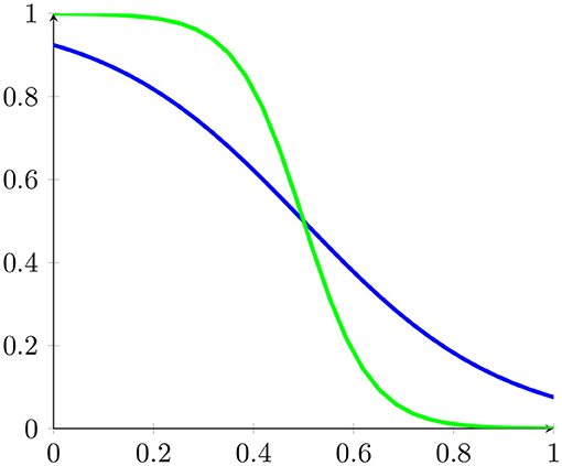
Figure 11. The sigmoid function $S(x)=\frac{1}{1+exp(\beta (x-0.5))}$ for β = 5 and β = 15.

Here β represents the inverse temperature of simulated annealing. This sigmoid function in the limit β → ∞ becomes the function

$S(x)=\{\begin{array}{cc}1& \text{when}x<1/2,\\ 0& \text{when}x>1/2,\\ 1/2& \text{when}x=1/2.\end{array}$

The simulated annealing program finds the system of weights presented in Table 5. For comparison, in Table 6 we find a system of weights for the handcrafted Algorithm 3.

TABLE 6

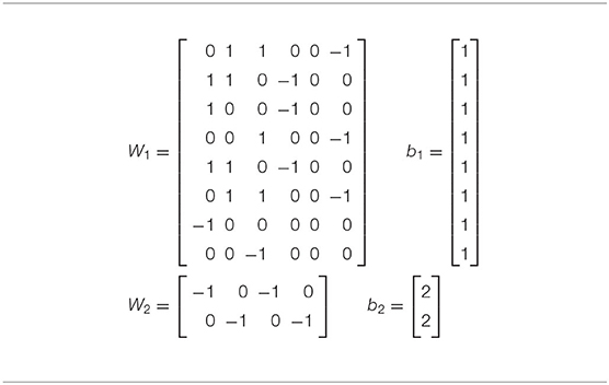
Table 6. Optimal weights found by reading them off from the handcrafted decoder (Algorithm 3).

As it is seen, the energy was reduced to approximately 10⁻³ which is a guarantee that all responses have been correct. The outputs are presented alongside with inputs in Table 7. For comparison, the weights directly read from the program Algorithm 3 are in Figure 6. Clearly, the weights learned by simulated annealing differ from the handcrafted weights. However, they both reproduce equivalent results. Interestingly, both programs correctly decode output of the topological Markov chain presented in Figure 6, with approximately 500 frames. The sample constructed contains “stretched” characters 'X' and 'O' obtained by repeating falling and rising spans of random length. Thus, the weights constructed by simulated annealing learned how to solve the more general problem than indicated by the sole example used as a training set.

TABLE 7

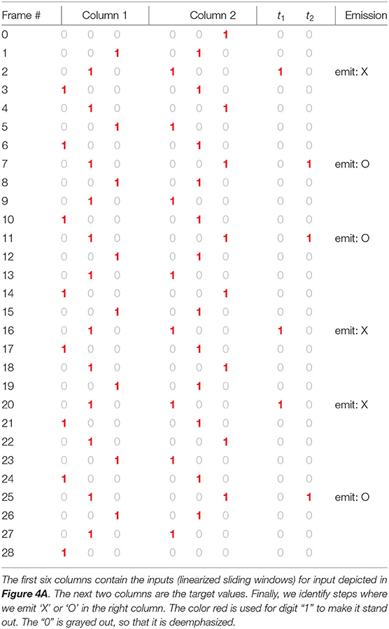
Table 7. The output of the simulator using optimal weights constructed by simulated annealing (Figure 5).

It should be noted that we search for a network with the same architecture as the network which we constructed by hand: inputs of length 6, outputs of length 2, and 4 memory cells. This perhaps made the search easier. However, it should also be noted that the search space has 48+8 = 56 weights and 8+2 = 10 biases. Since input weights are restricted to 3 values and biases to 6 values, the total search space has

$3^{56}·6^{10}\approx 3.16·10^{34}$

nodes. Thus, our search, which terminated in minutes, had a sizable search space to explore (some variations led to much quicker times, in the 10 second range). Furthermore, repeated searches found only 2 perfect solutions. It is quite possible that the number of solutions is very limited for the problem at hand, perhaps only a few.

In our solution we used a simple rule for state modification: we simply modified a random weight or bias, by randomly choosing an admissible value: {±1, 0} for weights and {0, 1, …, 5} for biases. The recommended rule is to try to stay at nearly the same energy, but for our example this did not seem to make significant difference for the speed or quality of the solution. At some point, we tried to tie the values of the biases to be the number of −1's in the corresponding row of the weight matrix, motivated by biases that come out of arithmetization of formulas of boolean logic. It turns out that this results in a significantly less successful outcome, and it appears important that the weights and biases can be varied independently.

9. Continuous Weights

In the current section we allow the weights of the deductron to be real numbers. As we can see, there is no need for β (the inverse temperature), as it can be easily absorbed by the weights. Similarly, the shift of 0.5 used in our falling sigmoid S [see (3)] can be absorbed by the biases. Also, we choose to use the standard, rising sigmoid function:

$\begin{array}{ll}\sigma (x)=\frac{1}{1+e^{-x}}.& (4)\end{array}$

This necessitates taking the complement of 1 when computing the output of the net.

The loss (error) function is simply the sum of squares of errors:

$\begin{array}{ll}loss={\displaystyle \sum _{f=1}^{n_{frames}}}{\displaystyle \sum _{i=1}^{n_{out}}}{\left(t_i^{(f)}-o_i^{(f)}\right)}^2.& (5)\end{array}$

Exercise 14 (Gradient of loss). Using Figure 10, find the gradient of the loss function given by (5) over the parameters. That is, find the formulas for the partial derivatives:

$\begin{array}{l}\frac{\partial loss}{\partial w_{ij}^{(k)}},\\ \frac{\partial loss}{\partial b_i^{(k)}},\end{array}$

where $W_k=\left[w_{ij}^{(k)}\right]$ and $b_k=\left[b_i^{(k)}\right]$, k = 1, 2 are the weight matrices and bias vectors of the deductron. ♠

The above exercise is important when one wants to implement a variation of Gradient Descent in order to find optimal weights and biases. The mechanics of differentiation are not particularly interesting. However, for complex neural networks it represents a challenge when implemented by manual application of the Chain Rule. Therefore, a technique called automatic differentiation is used, which essentially implements the Chain Rule in software. The computer manipulates the formulas expressing loss to obtain the gradient. The system Tensorflow [9] provides the facility to carry it out with a minimum amount of effort and allows for quick modification of the model. In contrast, the human would have to essentially repeat the calculations manually for each model variation, which inhibits experimentation.

Following the documentation of Tensorflow, we implemented training of a deductron RNN, closely following Figure 10. The implementation is available at GitHub [14].

Exercise 15 (Generating W-language samples with interval maps). Use the interval map in Figure 9 to generate samples of the W-language, like the one below:

Assume that the image begins and ends with exactly one blank (not shown). The image has exactly 155 columns. This sample should decode to the following decoded message, with 'X' and 'O' appearing at the time of their emission:

Use the samples generated with the interval map instead of the samples generated with a random number generator to train the Deductron to recognize the W-language. NOTE: You will have to slightly perturb the mapping of the interval, as multiplication by 2 and 4 leads to rapid decay of the precision on computers using base-2 arithmetic, ending in a constant sequence after several dozen of iterations. ♠

10. Computational Complexity of Gradient Evaluation

Ideally, we would have an a priori bound for the time complexity of some variant of Stochastic Gradient Descent (SGD) to approximate the optimum weights with prescribed accuracy. However, for most neural networks this is either impossible or not practical. Therefore, we must settle for estimating the computation cost of a step of SGD, which is predominantly the cost of finding the gradient itself.

Theorem 3 (On time complexity of deductron gradient). Let the input of the deductron in Figure 10 consist of frames of size n_in and let n_frames be the number of frames. Let L be a loss function similar to one given by (5). Let n_memory ≥ 1 be the number of memory cells. Let n_out be the size of the output frame. Then the time complexity of finding the gradient of loss with respect to the weights and biases, i.e., the cost of finding all quantities

$\frac{\partial loss}{\partial w_{ij}^{(k)}},\frac{\partial loss}{\partial b_i^{(k)}}$

is:

$\begin{array}{ll}O\left((n_{out}+·n_{in})·n_{memory}^2·n_{frames}^2\right).& (6)\end{array}$

Proof. Let v be a vector variable representing weights and biases. First, let us consider v = (W₁, b₁). When linearized, this vector has 2(n_memory·n_in+n_memory) entries. According to the Chain Rule (of vector calculus), the quantity

$\frac{\partial loss}{\partial v}$

is a sum of products of partial derivatives where the summation is over all paths connecting the variable v to the variable loss within the directed graph contained in Figure 10:

$\begin{array}{ll}\frac{\partial loss}{\partial v}=\frac{\partial loss}{\partial o_0}·\frac{\partial o_0}{\partial z_0}·\frac{\partial z_0}{\partial u_0}·\frac{\partial u_0}{\partial h_0}·\frac{\partial h_0}{\partial v}+\cdots & (7)\end{array}$

where the partials are, in fact, matrices (Jacobi matrices). We perform the multiplication from the left. In this manner, every one of the four matrix products is of a row vector on the left by a matrix on the right. The cost of the multiplication is thus approximately the product of the dimensions of the matrix on the right (sometimes the complexity is lower if the matrix is sparse, e.g., diagonal). The complexity of each entry of each of the matrices has constant time complexity. Therefore, the cost of computing the four matrix products above is estimated as follows:

$\begin{array}{l}{n}_{out}·n_{memory}+n_{memory}^2+n_{memory}+n_{memory}·(n_{memory}·n_{in}+n_{memory}).\end{array}$

Other terms in Equation (7) are estimated in the same manner. We note that loss is an implicit node in the graph, with an edge from o_j, j = 0, 1, …, n_frames − 1 to loss. It remains to note that the number of paths from v to loss is estimated by $n_{frames}^2$. Other terms of the sum (7) and the case v = (W₂, b₂), are handled in a similar manner. Formula (6) follows.     □

The above proof is general enough to be applicable to most RNN and a variety of loss functions. The proof makes it evident that the main cost of gradient computation comes from matrix multiplication, resulting in quadratic dependence on the size of memory. It also indicates that with a parallel model of computation the cost can be lowered, as matrix multiplication can be parallelized. Optimally the cost can be made linear in the number of columns of the underlying matrices, thus making complexity proportional to n_memory, not $n_{memory}^2$.

There is another corollary of Theorem 3, related to the presence factor $n_{frames}^2$. In principle, one could train an RNN using a single sequence, as we did, e.g., concatenating many samples of the W-language. However, from the point of view of complexity, it is better to keep independently collected samples in the training dataset separate, so that the number of frames remains as small as possible, and add the loss function across the samples.

Example 4 (Complexity of combining samples). Let us suppose we have k samples of W-language, each having n_frames frames. The combined sample has length k · n_frames and gradient cost is proportional to ${(k·n_{frames})}^2=k^2·n_{frames}^2$. The cost of computing gradients separately and adding them up is proportional to $k·n_{frames}^2$. Thus, the cost of combining k samples is larger by a factor of k. ♣

The cost of lengthy samples cannot be mitigated by parallelization. The problem is very similar to that of performing operations on sparse matrices using algorithms designed for dense matrices, e.g. matrix multiplication: we end up multiplying by 0 a lot. For RNN, by concatenating input samples we will compute terms in Equation (7) which are known to be 0.

11. Deductron and Applications

In general, RNN are mainly used to solve the problem of sequence-to-sequence mapping, such as the application to decoding the W-language presented in this paper. Another and more straightforward type of application is sequence-to-label mapping, in which an RNN is used for pattern classification. Our focus is on sequence-to-sequence mapping.

Sequence-to-sequence mapping applications of RNNs often combine the RNN with another machine learning technique called Connectionist Temporal Classification (CTC) [1, 2, 15–18]. For applications such as OCR of cursive scripts and speech and handwriting recognition, the combination RNN+CTC is in fact a de facto standard in most real systems of today. Therefore, the suitability of a particular RNN architecture as a general-purpose RNN architecture should be evaluated by its ability to cooperate with CTC.

We divide the application of the deductron into two categories:

1. Pure sequence-to-sequence mapping, which does not use CTC.

2. RNN used alongside with CTC.

Clearly, the main example in this paper (that of the W-language decoding) is in the first category. However, it is natual and desirable to combine deductron with CTC to decode the W-language, as it will be explained in the next subsection.

11.1. Deductron With CTC

Deductron in combination with CTC, along with LSTM, GRU and other neural nets, is currently being tested for use in a new OCR system Wordly Ocr [19]. Therefore, comprehensive side-by-side comparisons of these networks will soon be available. Small, demonstration-type applications will be ported to Python and placed in this paper's GitHub repository [14]. In this section we outline the way deductron is used with CTC. Most of the discussion is applicable to other RNNs, also.

The benefit provided by CTC is the ability to use naturally structured training data. An RNN, with or without CTC, maps sequences in one alphabet to sequences in another alphabet. However, without CTC both sequences must be of the same length (=number of frames). With CTC long sequences of frames can be mapped to sequences of different length.

Example 5 (W-language and CTC). When decoding images representing W-language expressions, such as the one in Figure 1, we combined two columns of an image of height 3 into a frame of height 6. Thus, a 3 × 30 image results in a sequence of 29 vectors of height 6. However, the sequence 'XOOXXO' has only 6 characters. ♣

With CTC we no longer need to instruct our network that symbols ('X' and 'O' for W-language) need to be emitted at a particular time steps. We can simply state what sequence should be emitted.

Some changes in the architecture and interpretation of the output of an RNN are needed to reap the benefits of CTC. The role of RNN changes when used as an RNN+CTC tandem. The output of the RNN is interpreted as a probability distribution of emitting a symbol of the alphabet at a given time (= frame number). An additional symbol is added to the alphabet, known as Graves' blank to be emitted when the network is undecided about the symbol that should be emitted.

Generation of the probability distribution is accomplished by using the softmax function, also known as the Boltzmann distribution or Gibbs distribution. The softmax function [see, for example, [20–22]] is defined as a mapping σ:ℝ^K → ℝ^K where

$\begin{array}{l}\sigma {(u)}_i=\frac{e^{u_i}}{{\displaystyle {\sum }_{j=1}^K}{e}^{u_j}}\end{array}$

and $u=(u_1,u_2,\dots ,u_K)\in {ℝ}^K$.

Example 6 (Graves' blank and W-language). In the main example of the W-language, the new alphabet, extended by the blank, has 3 elements:

${{A}}^{\prime }={A}\cup \left\{\text{\_}\right\}=\left\{\vee ,\wedge ,\text{\_}\right\}.$

Thus we use the underscore symbol '_' as Graves' blank. This symbol is emitted whenever we do not want to commit to emitting either 'X' or 'O'. The emission of '_' may occur in the gaps between 'X' and 'O' (runs of 0) or due to repeated vectors e_j, j = 1, 2, 3, or due to some kind of error. In order to use an RNN with CTC we must modify the output layer of the RNN to emit a probability distribution for every frame, rather than a symbol. For a sequence of T = 29 frames of height 6, the output is a matrix with non-negative entries:

$P=\left[\begin{array}{cccc}{p}_{1,X}& p_{2,X}& \dots & p_{T,X}\\ p_{1,O}& p_{2,O}& \dots & p_{T,O}\\ p_{1,\text{\_}}& p_{2,\text{\_}}& \dots & p_{T,\text{\_}}\end{array}\right].$

Every column $p_t=(p_{t,X},p_{t,O},p_{t,\text{\_}})\in {ℝ}^3$ is a probability vector. In particular, for t = 1, 2, …, T:

$\begin{array}{l}{p}_{t,X}+p_{t,O}+p_{t,\text{\_}}=1.\end{array}$

This leads to the following formula for the entries of the matrix P, computed in two steps:

o_t ← W₂z_t + b₂

p_t ← σ(o_t)

These steps are used in place of line 10 of Algorithm 7. This imposes the dimensions upon W₂ and b₂. The matrix W₂ is 3 × n_memory and $b_2\in {ℝ}^3$. ♣

The theory of CTC is beyond the scope of this paper. However, the technique is well-documented in a number of papers [17, 18, 23–25]. There is a variety of implementations, both standalone and as a part of a bigger system. For a quick programmer's introduction to CTC we recommend the short paper by Wang [25]. However, one needs to study the thesis of Graves [15] for a detailed exposition. We found that tackling numerical stability of the CTC algorithm is of paramount importance. In particular, for any serious application, such as OCR of cursive scripts (such as Arabic) it is necessary to perform probability calculations using logarithmic scale. This is to prevent underflow in performing floating point arithmetic, resulting from multiplication of many extremely small probabilities. This occurs in calculating the gradient of the loss, and is known as the vanishing gradient problem.

We have performed experiments indicating that a CTC layer can be successfully used with deductron. A simple CTC implementation in MATLAB, following Wantee Wang's paper [25] is provided as part of the open source OCR project Wordly Ocr [19, 26] and a demonstration program of CTC and LSTM used to decode W-language perfectly is provided. We also implemented a full production version of CTC in MATLAB which was used to perform OCR on Persian and Latin cursive script [27]. A complete example involving deductron and CTC will be posted to this paper's GitHub repository [14].

11.2. Deductron for Sequence-to-Sequence Mapping

Recently Dylan Murphy implemented deductron within the Keras framework [28] and re-wrote a demo application which originally uses LSTM layers to solve a pure sequence-to-sequence mapping problem [29]. His contribution is available in this paper's GitHub repository [14]. Using this implementation, the author added a Python program demonstrating that deductron can be successfully used to replace LSTM completely, and achieve accuracy of 99.5% on the same problem, similar to that obtained with LSTM.

Let us briefly describe the problem and the form of training data. The task is to teach a computer addition of non-negative decimal integers from examples. Thus, we prepare training data in the form of input/target pairs, e.g., “535+61=596” (a string). The alphabet in this example is '0123456789+'.

The approach taken by the original authors of the example splits the problem into two subproblems:

1. Encoding; the numbers to be added are converted to one-hot encoding; the numbers are added in the one-hot (unary) representation;

2. Decoding; the result is translated back to a string representation using decimal digits.

Both subproblems are solved using RNN. In the original code by the Keras team, the RNN is LSTM. We found that LSTM can be replaced with deductron and achieve comparable results:

1. In the decoder role, a single deductron replaces an LSTM with the same number of hidden units (memory cells for deductron);

2. In the encoder role, an LSTM replacement consists of two deductrons arranged as consecutive elements in the pipeline, with a comparable number of trainable parameters (weights and biases) in the overall model.

The idea of replacing a single LSTM with two deductrons comes from the comparison of both architectures (cf. Figure 10 and Appendix). In LSTM, data is pushed through two Hadamard gates, while in deductron there is only one non-linearity in the V-gate, aside from the perceptron layers present in both LSTM and deductron.

12. Additional Research Notes and Future Directions

There are also indications that deductron, as described in this paper, has some limitations when the input sequences have complex grammatical rules. This appears to be due to the fact that deductron is stateless, i.e., the memory is not initialized in any particular way. Therefore, its “wisdom” is encapsulated in the weights of the perceptron layers embedded into the deductron. Making deductron stateful is an interesting research direction. For example, instead of initializing memory with 0 we can use a learnable parameter ROM (“read-only memory”). This would allow deductron to retain some knowledge permanently, in addition to the knowledge stored in weights and biases.

13. Conclusions

In our paper we constructed a non-trivial and mathematically rigorous example of a class of image data representing encoded messages which requires long-term memory to decode.

We constructed a conventional computer program for decoding the data. The program was then translated to a Recurrent Neural Network. Subsequently, we generalized the neural network to a class of neural networks, which we call deductrons. A deductron is called that because it is a 3-layer neural network with a middle layer capable of simple inferences.

Finally, we demonstrated that our neural networks can be trained by using global optimization methods. In particular, we demonstrated that simulated annealing discovers an algorithm which decodes the class of inputs with 100% accuracy, and is logically equivalent to our first handcrafted program. We also showed how to train deductrons using Tensorflow and Adam optimizer.

Our analysis opens up a direction of research on RNNs which have more clear semantics than other RNNs, such as LSTM, with a possibility of better insight into the workings of the optimal programs. It is to be determined whether our RNN is more efficient than LSTM. We conjecture that the answer is “yes” and that our architecture is a class of RNN which can be trained faster and understood better from the theoretical standpoint.

Author Contributions

The author confirms being the sole contributor of this work and has approved it for publication.

Conflict of Interest

The author declares that the research was conducted in the absence of any commercial or financial relationships that could be construed as a potential conflict of interest.

Acknowledgments

This manuscript has been released as a pre-print at arXiv.org [30].

References

1. Graves A, Schmidhuber J. Offline handwriting recognition with multidimensional recurrent neural networks. In: Koller D, Schuurmans D, Bengio Y, Bottou L, editors. NIPS. Curran Associates, Inc. (2008). p. 545–52. Available online at: http://dblp.uni-trier.de/db/conf/nips/nips2008.html#GravesS08.

Google Scholar

2. Lipton ZC, Berkowitz J, Elkan C. A Critical Review of Recurrent Neural Networks for Sequence Learning. (2015). Available online at: http://arxiv.org/abs/1506.00019v4; http://arxiv.org/pdf/1506.00019v4.

Google Scholar

3. Yu Y, Si X, Hu C, Zhang J. A review of recurrent neural networks: LSTM cells and network architectures. Neural Comput. (2019) 31:1235–70. doi: 10.1162/neco_a_01199.

PubMed Abstract | CrossRef Full Text | Google Scholar

4. Salehinejad H, Sankar S, Barfett J, Colak E, Valaee S. Recent advances in recurrent neural networks. arXiv preprint. (2017). arXiv:180101078.

Google Scholar

5. Alom MZ, Taha TM, Yakopcic C, Westberg S, Sidike P, Nasrin MS, et al. A state-of-the-art survey on deep learning theory and architectures. Electronics. (2019) 8:292. doi: 10.3390/electronics8030292

CrossRef Full Text | Google Scholar

6. Hochreither S, Schmidhuber J. Long short-term memory. Neural Comput. (1997) 9:1735–80.

PubMed Abstract | Google Scholar

7. Gers FA, Schmidhuber J, Cummins FA. Learning to forget: continual prediction with LSTM. Neural Comput. (2000) 12:2451–71. doi: 10.1162/089976600300015015

PubMed Abstract | CrossRef Full Text | Google Scholar

8. Fan F, Xiong J, Wang G. On interpretability of artificial neural networks. abs/2001.02522 (2020).

Google Scholar

9. Abadi M, Agarwal A, Barham P, Brevdo E, Chen Z, Citro C, et al. TensorFlow: Large-Scale Machine Learning on Heterogeneous Systems. (2015). Software available from tensorflow.org. Available online at: https://www.tensorflow.org/.

Google Scholar

10. Kingma DP, Ba J. Adam: a method for stochastic optimization. ArXiv. (2014). Available online at: http://adsabs.harvard.edu/abs/2014arXiv1412.6980K.

Google Scholar

11. Mackay DJC. Information Theory, Inference and Learning Algorithms. Cambridge, UK: Cambridge University Press (2003).

Google Scholar

12. Knuth DE. The Art of Computer Programming, Volume 2 (3rd Ed.): Seminumerical Algorithms. Boston, MA: Addison-Wesley Longman Publishing Co., Inc. (1997).

Google Scholar

13. Alligood KT, Sauer TD, Yorke JA. Chaos: An Introduction to Dynamical Systems. Textbooks in Mathematical Sciences. New York, NY: Springer (2000). Available online at: https://books.google.com/books?id=48YHnbHGZAgC.

Google Scholar

14. Rychlik M. DeductronCode. Contains contributions by Dylan Murphy (2020). Available online at: https://github.com/mrychlik/DeductronCode.

15. Graves A. Supervised Sequence Labelling With Recurrent Neural Networks. Technical University Munich (2008). Available online at: https://www.bibsonomy.org/bibtex/2bf7c42c76bd916ced188d112f130b608/dblp.

Google Scholar

16. Sankaran N, Jawahar CV. Recognition of printed Devanagari text using BLSTM Neural Network. In: Proceedings of the 21st International Conference on Pattern Recognition (ICPR2012) (Tsukuba) (2012). p. 322–5.

Google Scholar

17. Kraken (2018). Available online at: http://kraken.re/ (accessed November 24, 2019).

18. Tesseract Open Source OCR Engine (main repository) (2018). Available online at: https://github.com/tesseract-ocr/tesseract.

19. Worldly-OCR GitHub repository (2018). Available online at: https://github.com/mrychlik/worldly-ocr (accessed November 24, 2019).

20. Wikipedia. Softmax Function. (2020). Available online at: https://en.wikipedia.org/wiki/Softmax_function (accessed November 24, 2019).

21. Rychlik M. A proof of convergence of multi-class logistic regression network. arXiv preprints. (2019). Available online at: https://arxiv.org/abs/1903.12600.

Google Scholar

22. Bishop CM. Neural Networks for Pattern Recognition. New York, NY: Oxford University Press, Inc (1996).

Google Scholar

23. Graves A. Generating sequences with recurrent neural networks. CoRR abs/1308.0850 (2013).

Google Scholar

24. Zyrianov S. rnnlib. Work derived from A. Graves' original implementation (2020). Available online at: https://github.com/szcom/rnnlib.

Google Scholar

25. Wang W. RNNLIB: Connectionist Temporal Classification and Transcription Layer. (2008). Available online at: http://wantee.github.io/assets/printables/2015-02-08-rnnlib-connectionist-temporal-classification-and-transcription-layer.pdf.

26. Keras Team. W-Language With LSTM and CTC (2020). Available online at: https://github.com/mrychlik/worldly-ocr/tree/master/WLanguageWithCTC (accessed November 24, 2019).

27. Rychlik M, Nwaigwe D, Han Y, Murphy D. Development of a New Image-to-text Conversion System for Pashto, Farsi and Traditional Chinese. Machine Learning and Big Data Approach. Submitted as part of a project report to the National Endowment for Humanities (2020). Available online at: https://securegrants.neh.gov/publicquery/main.aspx?f=1&gn=PR-263939-19.

Google Scholar

28. Team Keras. Keras: The Python Deep Learning API (2020). Available online at: https://keras.io/ (accessed November 24, 2019).

29. Wikimedia Commons. An Implementation of Sequence to Sequence Learning for Performing Addition (2020). Available online at: https://keras.io/examples/nlp/addition_rnn/.

30. Rychlik M. Deductron – A recurrent neural network. arXiv preprint. arXiv: 1806.09038 (2018).

Google Scholar

31. Keras Team. File:Peephole Long Short-Term Memory.svg — Wikimedia Commons, the Free Media Repository (2017). Available online at: https://commons.wikimedia.org/w/index.php?title=File:Peephole_Long_Short-Term_Memory.svg&oldid=247762287 (accessed June 20, 2018).

14. Appendix

14.1. Peephole LSTM Architecture

The flow of data in an LSTM is illustrated by the following diagram [31]:

The formulas expressing the data transformations are:

$\begin{array}{ll}{f}_t={\sigma }_g(W_f{x}_t+U_f{c}_{t-1}+b_f)& (\mathrm{A1})\end{array}$

$\begin{array}{ll}{i}_t={\sigma }_g(W_i{x}_t+U_i{c}_{t-1}+b_i)& (\mathrm{A2})\end{array}$

$\begin{array}{ll}{o}_t={\sigma }_g(W_o{x}_t+U_o{c}_{t-1}+b_o)& (\mathrm{A3})\end{array}$

$\begin{array}{ll}{c}_t=f_t◦c_{t-1}+i_t◦{\sigma }_c(W_c{x}_t+b_c)& (\mathrm{A4})\end{array}$

$\begin{array}{ll}{h}_t=o_t◦{\sigma }_h(c_t)& (\mathrm{A5})\end{array}$

Every quantity is a vector. The symbol “◦” stands for the Hadamard (elementwise) product. Thus, to perform the product, the vectors have to have the same length. The functions σ_∗ are sigmoid activation functions.