Reconstructing Complex Cardiac Excitation Waves From Incomplete Data Using Echo State Networks and Convolutional Autoencoders

1 Introduction

Cardiac arrhythmias, such as ventricular or atrial fibrillation, are electro-mechanical dysfunctions of the heart that are associated with complex, chaotic spatio-temporal excitation waves within the heart muscle resulting in incoherent mechanical contraction and a significant loss of pump function [1–3]. Ventricular fibrillation (VF) is the most common deadly manifestation of a cardiac arrhythmia and requires immediate defibrillation using high-energy electric shocks. Atrial fibrillation (AF) is the most common form of a cardiac arrhythmia, affecting 33 million patients worldwide [62]. While not immediately life-threatening, AF is considered to be responsible for 15% of strokes if left untreated [63, 64]. The structural substrate and functional mechanisms that underlie the onset and perpetuation of VF and AF are not fully understood. It is generally agreed that imaging of the cardiac electrical and mechanical function is key to an improved mechanistic understanding of cardiac disease and the development of novel diagnosis and therapy. This has motivated the development of non-invasive and invasive electrophysiological measurement and imaging modalities. Electrical activity of the heart can (so far) non-invasively be measured on its surface, only. Direct measurements can be made in vivo inside the heart using so-called basket catheters with typically 64 electrodes or in ex-vivo experiments, where an extracted heart in a Langendorff perfusion set-up is kept beating and the cell membrane voltage on the epicardial surface is made visible using fluorescent dyes (a method also known as optical mapping) [4]. A method for indirect observation of electrical excitation waves is ECG imaging where an array of EEG-electrodes is placed on the body surface and an (ill-posed) inverse problem is solved to estimate the potential on the surface of the heart. Mechanical contraction and deformation of the heart tissue can be studied in full 3D using ultrasound, in 2D using real-time MRT [5] or (using optical mapping) by motion tracking in Langendorff experiments.

The reconstruction of patterns of action potential wave propagation in cardiac tissue from ultrasound has been introduced by Otani et al. [6, 7]. They proposed to use ultrasound to visualize the propagation of these waves through the mechanical deformations they induce and to reconstruct action potential-induced active stress from the deformation. Provost et al. [8] introduced electromechanical wave imaging to map the mechanical deformation of cardiac tissue at high temporal and spatial resolutions. The observed deformations resulting from the electrical activation were found to be closely correlated with electrical activation sequences. The cardiac excitation-contraction-coupling (ECC) [9] has also been studied in optical mapping experiments in Langendorff-perfused isolated hearts [10–12]. Using electromechanical optical mapping [12], it was shown that during ventricular tachyarrhythmias electrical rotors introduce corresponding rotating mechanical waves. These co-existing electro-mechanical rotors were observed on the epicardial surface of isolated Langendorff-perfused intact pig and rabbit hearts using optical mapping [13]. Using high-resolution ultrasound, these mechanical rotors were also observed inside the ventricular wall during ventricular tachycardia and fibrillation [13].

All these measurement modalities are limited, in particular those suitable for in vivo applications. Measurements with basket catheters are effectively undersampling the spatio-temporal wave pattern. Inverse ECGs suffer from ill-posedness and require regularization that may lead to loss of spatial resolution and blurring. Limited spatial resolution is also an issue with ultrasound measurements, but they are currently the only way to “look inside” the heart, albeit measuring only mechanical motion. Electrical excitation waves inside the heart muscle are so far not accessible by any measurement modality available.

These limitations motivated the search for algorithms to reconstruct electro-mechanical wave dynamics in cardiac tissue from measurable quantities. Berg et al. [14] devised synchronization-based system identification of extended excitable media, in which model parameters are estimated by minimizing the synchronization error. Using this approach, Lebert and Christoph [15] demonstrated that electro-mechanic wave dynamics of excitable-deformable media can be recovered from a limited set of observables using a synchronization-based data assimilation approach. Hoffman et al. reconstructed electrical wave dynamics using ensemble Kalman filters [16, 17]. In another approach, it was shown that echo state networks [18] and deep convolutional neural networks [19, 20] provide excellent cross estimation results for different variables of a mathematical model describing complex electrical excitation waves during cardiac arrhythmias. Following this approach, Christoph and Lebert [21] demonstrated the reconstruction of electrical excitation and active stress from deformation using a simulated deformable excitable medium. To continue this research and to address the general challenge of missing or impaired observations we consider in this article two tasks: (i) recovering electrical excitation patterns from noisy, blurred or undersampled observations and (ii) reconstructing electrical excitation waves from mechanical deformation. To solve the corresponding data processing and cross-prediction tasks two machine learning methods are employed and evaluated: echo state networks and convolutional autoencoders. Both algorithms are applied to synthetical data generated by prototypical models for electrophysiology and electromechanical coupling.

2 Methods

In this section we will first introduce in Sections 2.1 and 2.2 the mathematical models describing cardiac dynamics which were used to generate the example data for the two tasks to be solved: (i) recovering electrical wave pattern from impaired observations and (ii) cross-predicting electrical excitation from mechanical deformation. Then in Section 2.3 both machine learning methods used for solving these tasks, echo state networks (Section 2.3.1) and convolutional autoencoders (Section 2.3.2), will be briefly introduced.

2.1 Recovering Complex Spatio-Temporal Wave Patterns From Impaired Observations

For motivating, illustrating, and evaluating the employed methods for dealing with incomplete or distorted observations we shall use spatio-temporal time series generated with the Bueno-Orovio-Cherry-Fenton (BOCF) model [22] describing complex electrical excitation patterns in the heart during cardiac arrhythmias. The BOCF model is a set of partial differential equations (PDEs) with four variables and will be introduced in Section 2.1.1. In Section 2.1.2 a formal description of the data recovery tasks will be given.

2.1.1 Bueno–Orovio–Cherry–Fenton Model

Cardiac dynamics is controlled by electrical excitation waves triggering mechanical contractions of the heart. In the case of cardiac arrhythmias like lethal ventricular fibrillation, wave break-up and complex chaotic wave patterns occur resulting in significantly reduced pump performance of the heart. From the broad range of mathematical models describing this spatio-temporal dynamics [23] we chose the Bueno–Orovio–Cherry–Fenton (BOCF) model [22] to generate spatio-temporal time series that are used as a benchmark to validate our approaches for reconstructing complex wave patterns in excitable media from incomplete data. The BOCF model consists of four system variables whose evolution is given by four (partial) differential equations

$\begin{array}{l}\frac{\partial u}{\partial t}=D\cdot {\nabla }^{2}u-\left(J_{si}+J_{fi}+J_{so}\right)\hfill \\ \frac{\partial v}{\partial t}=\frac{1}{{\tau }_v^{-}}\left(1-H\left(u-{\theta }_v\right)\right)\left(v_{\infty }-v\right)-\frac{1}{{\tau }_v^{+}}H\left(u-{\theta }_v\right)v\hfill \\ \frac{\partial w}{\partial t}=\frac{1}{{\tau }_w^{-}}\left(1-H\left(u-{\theta }_w\right)\right)\left(w_{\infty }-w\right)-\frac{1}{{\tau }_w^{+}}H\left(u-{\theta }_w\right)w\hfill \\ \frac{\partial s}{\partial t}=\frac{1}{2{\tau }_s}\left(\left(1+\text{tanh}\left(k_s\left(u-u_s\right)\right)\right)-2s\right).\hfill \end{array}(1)$

The variable u represents the continuum limit representation of the membrane voltage of cardiac cells and the variables v, w, and s are gating variables controlling ionic transmembrane currents $J_{si}$, $J_{fi}$ and $J_{so}$ given by the equations

$\begin{array}{l}{J}_{si}=-\frac{1}{{\tau }_{si}}H\left(u-{\theta }_w\right)ws\\ J_{fi}=-\frac{1}{{\tau }_{fi}}vH\left(u-{\theta }_v\right)\left(u-{\theta }_v\right)\left(u_u-u\right)\\ J_{so}=\frac{1}{{\tau }_o}\left(u-u_o\right)\left(1-H\left(u-{\theta }_w\right)\right)+\frac{1}{{\tau }_{so}}H\left(u-{\theta }_w\right).\end{array}(2)$

Here $H(\cdot )$ denotes the Heaviside function and the currents depend on the following seven voltage controlled variables

$\begin{array}{l}{\tau }_v^{-}=\left(1-H\left(u-{\theta }_v^{-}\right)\right){\tau }_{v1}^{-}+H\left(u-{\theta }_v^{-}\right){\tau }_{v2}^{-}\\ {\tau }_w^{-}={\tau }_{w1}^{-}+\frac{1}{2}({\tau }_{w2}^{-}-{\tau }_{w1}^{-})(1+\tanh \left(k_w^{-}(u-u_w^{-})\right))\\ {\tau }_{so}^{-}={\tau }_{so1}+\frac{1}{2}({\tau }_{so2}-{\tau }_{so1})(1+\tanh \left(k_{so}(u-u_{so})\right))\\ {\tau }_s=(1-H(u-{\theta }_w)){\tau }_{s1}+H(u-{\theta }_w){\tau }_{s2}\\ {\tau }_o=(1-H(u-{\theta }_o)){\tau }_{o1}+H(u-{\theta }_o){\tau }_{o2}\\ v_{\infty }=\{\begin{array}{ll}1,\hfill & \text{if }u\le {\theta }_v^{-}\hfill \\ 0,\hfill & \text{if }u\ge {\theta }_v^{-}\hfill \end{array}\\ w_{\infty }=(1-H(u-{\theta }_o))(1-\frac{u}{{\tau }_{w\infty }})+H(u-{\theta }_o)w_{\infty }^{\ast }.\end{array}(3)$

For simulating the dynamics we used the set of parameters given in Table 1 for which the BOCF model was found [22] to exhibit excitation wave dynamics similar to the Ten Tusscher–Noble–Noble–Panfilov (TNNP) model [24] describing human heart tissue.

TABLE 1

TABLE 1. TNNP model parameter values for the BOCF model [22].

Typical snapshots of the four variables during a chaotic evolution are shown in Figure 1. The spatio-temporal chaotic dynamics of this system is actually transient chaos whose lifetime grows exponentially with system size [25, 26]. To obtain chaotic dynamics with a sufficiently long lifetime the system has been simulated on a domain of $512\times 512$ grid points with a grid constant of $\text{Δ}x=1.0$ space units and a diffusion constant $D=0.2$. Furthermore, an explicit Euler stepping in time with $\text{Δ}t=0.1$, a 5 point approximation of the Laplace operator, and no-flux boundary conditions were used for solving the PDEs.

FIGURE 1

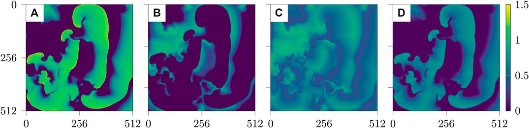
FIGURE 1. Snapshots of the four fields u, v, w, s of the BOCF model Eq. (1) (from left to right).

2.1.2 Reconstruction Tasks

Experimental measurements of the dynamics of a system of interest often allow only the observation of some state variables (e.g., the membrane voltage) and may provide only incomplete or distorted information about the measured observable. Typical limitations are (additive) measurement noise and low-spatial resolution (due to the experimental conditions and/or the available hardware). Formally, measurements impaired due to noise, blurring or undersampling can be described as follows: Let ${\mathbf{X}}_n\in {\mathrm{ℝ}}^{r\times c}$ be the measured data (here: snapshots of the field u) where r and c specify the two spatial dimensions. Each sample ${\mathbf{X}}_n$ with $n=1,\dots ,N$ corresponds to a true system output ${\mathbf{X}}_n^{\prime }\in {\mathrm{ℝ}}^{r^{\prime }\times c^{\prime }}$ that is assumed to be known only during the training phase in terms of a training set $\mathrm{}=\{{\mathbf{Z}}_1=({\mathbf{X}}_1,{\mathbf{X}}_1^{\prime }),\dots ,{\mathbf{Z}}_N=({\mathbf{X}}_N,{\mathbf{X}}_N^{\prime })\}$. Note that with coarse graining $r\le r{ }^{\prime }$ and $c\le c{ }^{\prime }$. The task is to predict the true system output ${\mathbf{X}}^{\prime }$ from impaired observations $\mathbf{X}$ which belong to one of the following three cases:

1. Noisy data: To add noise each element of ${\mathbf{X}}^{\prime }$ is replaced with probability p by 0 or 1 drawn from a Bernoulli distribution $\mathrm{ℬ}\left(0.5\right)$ (note that in our case ${\mathbf{X}}^{\prime }$ is given by the variable u of the BOCF model which has a range of $\left[\mathrm{0,1}\right]$). To simulate different levels of noise different probabilities $p=0.1,0.2,\dots ,0.9$ are used to generate noisy data sets $\left\{{\mathbf{X}}_n\right\}$. In the following p is called the noise level.

2. Blurred data: Date with reduced spatial resolution are obtained as Fourier low-pass filtered data $\mathbf{X}={\mathrm{ℱ}}^{-1}\left({\mathrm{}}^m\left(\mathrm{ℱ}\left({\mathbf{X}}^{\prime }\right)\right)\right)$ where $\mathrm{ℱ}$ and ${\mathrm{ℱ}}^{-1}$ denote the Fourier transform and its inverse, respectively, and ${\mathrm{}}^m$ is a projection where frequencies outside a radius $m\in [\mathrm{2,4,8},\dots ,18]$ (Manhattan distance) centered at frequency zero are set to zero.

3. Undersampled data: To generate undersampled date ${\mathbf{X}}^{\prime }$ is down-sampled ${\mathrm{ℝ}}^{r^{\prime }\times c^{\prime }}\to {\mathrm{ℝ}}^{r\times c}$ with $r<r^{\prime }$ and $c<c^{\prime }$ by accessing every 2ⁱ-th value of ${\mathbf{X}}^{\prime }$, where $i\in \left[\mathrm{1,7}\right]$.

Figure 2 shows examples of the three types of impaired observations.

FIGURE 2

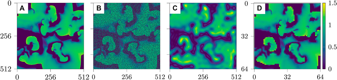
FIGURE 2. Snapshots of the three cases of impaired data based on u [from left to right: (A) reference data u, (B) noisy data, (C) blurred data, and (D) undersampled data].

2.2 Predicting Electrical Excitation From Mechanical Contraction

To learn the relation between mechanical deformation and electrical excitation inverse modelling data were generated by a conceptual electro-mechanical model consisting of an Aliev–Panfilov model describing the electrical activity and a driven mass-spring-system [15].

2.2.1 Aliev–Panfilov Model

Specifically developed to mimic cardiac action potentials in the myocardium, the Aliev–Panfilov model is a modification of the FitzHugh–Nagumo model, which reproduces the characteristic shape of electric pulses occurring in the heart [27]. It is given by a set of two differential equations,

$\frac{\partial u}{\partial t}=\nabla \left(\mathbf{D}\cdot \nabla u\right)-ku\left(u-a\right)\left(u-1\right)-uv(4)$

$\begin{array}{l}\frac{\partial v}{\partial t}=\mathit{ϵ}\left(u,v\right)\cdot \left(-v-ku\left(u-b-1\right)\right)\\ \mathit{ϵ}\left(u,v\right)={\mathit{ϵ}}_0+\frac{{\mu }_{1}v}{{\mu }_2+u}\end{array}(5)$

in which u and v are the normalized membrane voltage and the recovery variable, respectively, and a, b and k are model parameters. The term $\nabla \left(\mathbf{D}\cdot \nabla u\right)$ accounts for the diffusion, in which the tensor $\mathbf{D}$ can be used to model anisotropies in the myocardial tissue. In addition, the term $\mathit{ϵ}\left(u,v\right)$ is introduced to adjust the shape of the restitution curve by modulating the parameters ${\mu }_1$ and ${\mu }_2$. The computational advantage of the Aliev–Panfilov model lies in its simplicity over other ion-flow-based models which allows shorter runtimes and combined with the elastomechanical model, keeps computational costs fairly reasonable. For this reason, the Aliev–Panfilov model was chosen for generating synthetic data from complex chaotic electromechnical wave dynamics.

Within the heart muscle, the myocardium, cells contract upon electrical excitation through a passing action potential. At this point it is important to note that muscle fibre contracts along its principal orientation which has to be considered during the implementation of the mechanical part of the simulation. To couple the mechanical contraction of the muscle fibre to electrical excitation of a cell, as an extension to the Aliev–Panfilov model the active stress$T_a$ was introduced by Nash and Panfilov [28] which leads to contraction in the principal orientation of the muscle fibre. The change of the active stress is described by

$\frac{\partial T_a}{\partial t}={\mathit{ϵ}}_T\left(u\right)\cdot (k_{T}u-T_a) ,(6)$

where $k_T$ controls the strength of the build-up of active stress. The term ${\mathit{ϵ}}_T\left(u\right)$ regulates the influence of u on $T_a$ for large u. In our simulations we use a smooth function introduced by Göktepe and Kuhl [29] given by

${\mathit{ϵ}}_T(u)={\mathit{ϵ}}_{T,0}+({\mathit{ϵ}}_{\infty }-{\mathit{ϵ}}_{T,0})\cdot \text{exp}(-\text{exp}(-{\xi }_T\cdot (u-u_0)) .(7)$

Here, ${\xi }_T$ controls the steepness of the transition between ${\mathit{ϵ}}_{\infty }$ and ${\mathit{ϵ}}_{T,0}$ and $u_0$ denotes the potential threshold for the activation of the active stress, with ${\mathit{ϵ}}_{\infty }<{\mathit{ϵ}}_{T,0}$ to achieve a physiological time course [30].

2.2.2 Mass-Spring Damper System

The elasto-mechanical properties of the cardiac muscle fibre were implemented using a modified two-dimensional mass-spring damper system [31]. For the current study the mass-spring system was implemented in two dimensions because this allows shorter runtimes and primarily serves as a proof-of-principle for the evaluated reconstruction approach. In its two-dimensional form this mechanical model might correspond best to a cut-out of the atrium’s wall, since there the muscle tissue is less than 4 mm thick. However, this mass-spring system can easily be expanded to three dimensions (see [15]).

Placed on a regular lattice, one mechanical cell is made up of four particles $x_i$ at the corners connected by structural springs and two sets of orthogonal springs connecting the centre of mass ${\overrightarrow{x}}_{\text{cm}}$ to each side of the cell (see Figure 3). The springs in the middle of the cell are called axial springs, of which one is made to be active (red). Here it is important to point out that one cell in the electrical model corresponds to one cell in the mechanical mass-spring system. For setting the fibre orientation through the active axial spring, the orientation parameter $\eta \in \left[\mathrm{0,1}\right]$ has been introduced, with which the four points of attachment $q_i$ can be computed easily. This parameter can be set individually for each cell, so that various fibre orientations can be modelled.

FIGURE 3

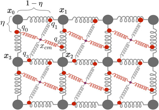
FIGURE 3. Two dimensional mass-spring damper system with one active spring modelling fibre orientation (red) and one passive spring (gray), the centre of mass $x_{\text{cm}}$, the four points of attachment $q_i$ to the structural springs and the orientation parameter η.

Using ${\overrightarrow{x}}_{\text{cm}}=\frac{1}{4}{{{\displaystyle \sum }}^{\text{}}}_{i=0}^3{\overrightarrow{x}}_i$ the forces from the passive spring ${\overrightarrow{f}}_j$ and the active spring ${\overrightarrow{f}}_a$ are obtained as.

${\overrightarrow{f}}_j=-k_j(\parallel {\overrightarrow{q}}_j-{\overrightarrow{x}}_{\text{cm}}\parallel -l_{j,0})\cdot {\overrightarrow{e}}_j ,(8)$

${\overrightarrow{f}}_a=-k_a\left(\parallel {\overrightarrow{q}}_a-{\overrightarrow{x}}_{\text{cm}}\parallel -\frac{l_{a,0}}{1+c_a\cdot T_a}\right)\cdot {\overrightarrow{e}}_a .(9)$

Here $l_{j,0}$, $k_j$ and $l_{a,0}$, $k_a$ denote the resting lengths and spring constants of the passive and active spring, respectively. From Eq. (9) it can be seen that, upon a rise in active stress $T_a$ from Eq. (6), the active spring contracts and an inward force is generated. The parameter $c_a$ represents a scaling factor to modulate the influence of the active stress. Through the orientation parameter the forces from the active and passive spring can be redistributed to the corresponding particles at the corners. For example for ${\overrightarrow{q}}_1$, the force on $x_0$ would be ${\overrightarrow{f}}_0=\eta {\overrightarrow{f}}_{q_1}$ and on $x_1$ it would amount to ${\overrightarrow{f}}_1=\left(1-\eta \right){\overrightarrow{f}}_{q_1}$.

In addition, the mechanical grid is held together by structural forces between the corner particles, which can be computed using

${\overrightarrow{f}}_{ij}=-k_{ij}(\parallel {\overrightarrow{x}}_i-{\overrightarrow{x}}_j\parallel -l_{ij})\cdot {\overrightarrow{e}}_{ij} ,(10)$

${\overrightarrow{f}}_{ji}=-{\overrightarrow{f}}_{ij} ,(11)$

with $l_{ij}$ being the resting length between particle $x_i$ and $x_j$.

Finally, with all the above forces acting on particle $x_i$ with mass $m_i$, its motion is determined according to

$m_i\frac{{\text{d}}^2{\overrightarrow{x}}_i}{\text{d}{t}^2}={\displaystyle \sum }_{\left\{a\right\}\left\{j\right\}\left\{ij\right\}}\overrightarrow{f_k}-\nu \frac{\text{d}{\overrightarrow{x}}_i}{\text{d}t} ,(12)$

with the sum ${\displaystyle \sum }_{\left\{a\right\}\left\{j\right\}\left\{ij\right\}}\overrightarrow{f_k}$ of all relevant springs pulling or pushing the particle. The damping constant ν sets the strength of the damping to increase the stability of the mechanical system as a whole.

The area of each cell was calculated with a simple formula for a general quadrilateral using the positions of its four corners. As a measure of contraction, the relative change of area

$\text{Δ}A\left(t\right)=\frac{A\left(t\right)}{A_{\text{undeformed}}}-1(13)$

has been used. The numerical algorithm for solving the full set of electro-mechanical ODEs is summarized in the Appendix.

2.2.3 Reconstruction Task

The inverse modelling data are generated by forward modelling $M:u\mapsto \text{Δ}A$ using the output of Equations (4) and (13). The task is to train an ESN or CAE to approximate $M^{-1}:\text{Δ}A\mapsto u$. To fulfill this task we use the membrane voltages and the local deformations at all $r\times c$ grid points sampled at times $t_n$. The training data set $\mathrm{}=\{{\mathbf{Z}}_1=({\mathbf{X}}_1,{\mathbf{X}}_1^{\prime }),\dots ,{\mathbf{Z}}_N=({\mathbf{X}}_N,{\mathbf{X}}_N^{\prime })\}$ thus consists of snapshots ${\mathbf{X}}_n\in {\mathrm{ℝ}}^{r\times c}$ and ${\mathbf{X}}_n^{\prime }\in {\mathrm{ℝ}}^{r\times c}$ of the relative mechanical deformation $\text{Δ}A\left(t_n\right)$ and the membrane voltage $u\left(t_n\right)$, respectively, and we aim at approximating $M^{-1}:{\mathbf{X}}_n\mapsto {\mathbf{X}}_n^{\prime }$ with $r,c=100$.

2.3 Machine Learning Methods

In this section we will introduce the two machine learning approaches, echo state networks (ESN) [32] and convolutional autoencoders (CAE) [33], that will be applied to solve the reconstruction tasks defined in Section 2.1.2.

2.3.1 Echo State Network

Echo state networks have been introduced in 2001 by Jaeger [32] as a simplified type of recurrent neural network, in which the weights describing the strength of the connections within the network are fixed. In its general composition an ESN subdivides into three sections [32], as illustrated in Figure 4. First of all, there is the input layer into which the input signal ${\overrightarrow{u}}_n\in {\mathrm{ℝ}}^{N_u}$ and a constant bias $b_{in}$ are fed. Secondly, the intermediate reservoir consists of N nonlinear units and its state is given by ${\overrightarrow{s}}_n\in {\mathrm{ℝ}}^N$. And lastly, the output layer provides the output signal ${\overrightarrow{y}}_n\in {\mathrm{ℝ}}^{N_y}$. Here, n denotes the discrete time steps $n=1,\dots ,T$.

FIGURE 4

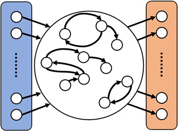
FIGURE 4. Schematic representation of an ESN. On the left side (colored in blue) is the input layer where the input signal ${\overrightarrow{u}}_n$ and a constant bias $b_{in}$ are fed in. The reservoir is represented as the large circle in the middle, where the small circles are the nodes. The output layer on the right (colored in orange) provides the reservoir signals ${\overrightarrow{s}}_n$ that are part of the vector ${\overrightarrow{x}}_n=[b_{out};{\overrightarrow{s}}_n;{\overrightarrow{u}}_n]$ used for computing the output ${\overrightarrow{y}}_n={\mathbf{W}}_{\text{out}}{\overrightarrow{x}}_n$.

The concatenated bias-input vector $[b_{in};{\overrightarrow{u}}_n]$ is fed into the reservoir through the input matrix ${\mathbf{W}}_{in}\in {\mathrm{ℝ}}^{N\times \left(1+N_u\right)}$. Inside the reservoir connections are given by the weight matrix $\mathbf{W}\in {\mathrm{ℝ}}^{N\times N}$, where N is the reservoir size. Together with the input matrix it is possible to determine the state of the reservoir at time n through the update rule

${\overrightarrow{s}}_n=(1-\alpha ){\overrightarrow{s}}_{n-1}+\alpha f_{in}({\mathbf{W}}_{in}[b_{in};{\overrightarrow{u}}_n]+\mathbf{W}{\overrightarrow{s}}_{n-1}) ,(14)$

in which $[\cdot ;\cdot ]$ denotes a concatenated vector. The input bias $b_{in}$, as well as the later introduced output bias $b_{out}$ were both set to 1 in the following. The parameter $\alpha \in (\mathrm{0,1}]$ in Eq. (14) represents the leaking rate which controls how much of a neuron’s activation is carried over to the next time step and can be used as a parameter to enhance predictions. As for the transfer function $f_{in}(\cdot )$ we use $\text{tanh}(\cdot )$ and the network dynamics used has no feedback loop. Only the weights ${\mathbf{W}}_{out}$ providing the output signal

${\overrightarrow{y}}_n={\mathbf{W}}_{out}{\overrightarrow{x}}_n\text{with}{\overrightarrow{x}}_n=[b_{out};{\overrightarrow{s}}_n;{\overrightarrow{u}}_n](15)$

are adapted during the training process by minimizing the cost function [34]

$C\left({\mathbf{W}}_{out}\right)={\displaystyle \sum }_n{\left|\left|{\overrightarrow{y}}_n^{true}-{\mathbf{W}}_{out}{\overrightarrow{x}}_n\right|\right|}^2+\lambda \text{Tr}\left({\mathbf{W}}_{out}{\mathbf{W}}_{out}^T\right)(16)$

where Tr denotes the trace of a matrix and λ controls the impact of the regularization term that prevents overfitting [35]. The final output matrix is given by the minimum of the cost function at ${\mathbf{W}}_{out}=\mathbf{Y}{\mathbf{X}}^{\text{T}}{\left(\mathbf{X}{\mathbf{X}}^{\text{T}}+\lambda 1\right)}^{-1}$ where $\mathbf{X}$ and $\mathbf{Y}$ are matrices whose columns are given by the vectors ${\overrightarrow{x}}_n$ and ${\overrightarrow{y}}_n^{true}$, respectively.

Both matrices ${\mathbf{W}}_{in}$ and $\mathbf{W}$, are initialized with random values from the interval $[-0.5,0.5]$. Since in experiments it turned out that more diverse dynamics could be modelled using networks in which only a small percentage $\mathit{ϵ}$ of weights inside the reservoir remained non-zero [32], the weight matrix $\mathbf{W}$ is made sparse with only a portion $\mathit{ϵ}$ of its values remaining non-zero. Furthermore, it is scaled by a factor $\frac{\rho }{\left|{\mu }_{max}\right|}$ where $\left|{\mu }_{max}\right|$ denotes here the largest eigenvalue of $\mathbf{W}$ and ρ is a hyperparameter for optimizing the performance (by ensuring the so-called echo state property [36]). To reduce the probability of drawing an dysfunctional set of matrix entries the randomly generated matrices ${\mathbf{W}}_{in}$ and $\mathbf{W}$ were selected from four different realisations. To optimize the performance of the ESN five hyperparameters ($N,\mathit{ϵ},\rho ,\alpha$ and λ) are tuned.

Reservoir computing using ESNs for predicting chaotic dynamics has already been demonstrated in 2004 by Jaeger and Haas [37]. Since then many studies appeared analyzing and optimizing this approach (see, for example [38–44], and references cited therein). In particular, it has been pointed out how reservoir computing exploits generalized synchronization of uni-directionally coupled systems [45, 46].

Recently, applications of ESNs to spatio-temporal time series have been presented [18, 47] employing many networks operating in parallel at different spatial locations based on the concept of (reconstructed) local states [48]. In particular, using this mode of reservoir computing it was possible to perform a cross-prediction between the four different variables of the BOCF model [18]. Therefore, for the current task of reconstructing data from impaired observations we build on the previous ESN design and modelling procedure. For each pixel an ESN is trained receiving input from neighboring pixels, only, representing the local state at the location of the reference pixel as illustrated in Figure 5. This design introduces two new hyperparameters σ and $\text{Δ}\sigma$ to the default ESN, where σ is the size of the stencil to define the local state and $\text{Δ}\sigma$ specifies the spatial distance of adjacent pixels included in the local state. Optimal values for all hyperparameters are determined by a grid search.

FIGURE 5

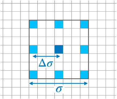
FIGURE 5. Stencil for locally sampling data used as input of the ESN operating at the location of the dark blue pixel in the center. The stencil is characterized by its width σ and the spatial separation $\Delta \sigma$ of sampling points.

2.3.2 Convolutional Autoencoder

A convolutional autoencoder [33] is a special architecture of a feed forward network (FFN) with convolutional layers similar to convolutional neural networks (CNNs) [49]. Generally a CAE learns a representation of the training set $\mathrm{}$ with the purpose of dimensionality reduction. For each pair ${\mathbf{Z}}_{\mathbf{i}}=\left({\mathbf{X}}_{\mathbf{i}},{\mathbf{X}}_{\mathbf{i}}^{\prime }\right)\in \mathrm{}$ the CAE is trained to perform a nonlinear transformation from the input representation of ${\mathbf{X}}_i$ to the output representation of ${\mathbf{X}}_i^{\prime }$. Like CNNs a CAE is a partially locally connected feed forward network, which is typically composed of the following layers:

Convolutional layers: Convolution of the input by a kernel sliding over the input. The number of rows and columns of the kernel are hyper-parameters, in this work they are set to be $3\times 3$.

Batch normalization layer: Normalization of the activations of the previous layer during training and for each batch. Batch normalization allows the use of higher learning rates, being computationally more efficient, and also acts as a regularizer [50].

Leaky ReLU [51] layer: Leaky version of a rectified linear unit (ReLU) [52], such that:

$\nu \left(x\right)=\{\begin{array}{cc}\alpha x\text{ for }x<0& \\ x\text{ for }x\ge 0.& \end{array}$

Max pooling layer: Sample-based operation for discretization based on a kernel that slides over the input like the convolutional operator but only the maximum value of the kernel is passed to the next layer. Width and height of the kernel are hyper-parameters (in this work $2\times 2)$. In contrast to the convolutional layer a pooling layer is not trainable.

Dropout layer: Regularization method to prevent overfitting where during training some weights are set randomly to zero [53]. In this work the probability of setting the weights to zero is 0.05.

The eponymous part of the CAEs are the convolutional layers, a convolution of $A=\left(a_{ij}\right)\in K^{n\times n}$ with a kernel $F=\left(f_{ij}\right)\in K^{k\times k}$, where $k<n$, is given by:

${\left(A\ast F\right)}_{xy}={\displaystyle \sum }_{i=-k/2}^{k/2}{\displaystyle \sum }_{j=-k/2}^{k/2}{a}_{xy}{f}_{\left(i-x\right)\left(j-y\right)},(17)$

with $x,y\in 1,\dots ,n$. If $i-x-$ or $j-y$ exceeds the range of A zero-padding is applied [54].

In this work two architectures are used. The first one employed to reconstruct the data from noisy, blurred and inverse modelling data is illustrated in Figure 6. The architecture is the same for the tasks in Section 2.1.2 and Section 2.2.3 but the sizes of $\mathbf{X}$ and ${\mathbf{X}}^{\prime }$ are different, with $\mathbf{X},{\mathbf{X}}^{\prime }\in {\mathrm{ℝ}}^{512\times 512}$ and $\mathbf{X},{\mathbf{X}}^{\prime }\in {\mathrm{ℝ}}^{100\times 100}$, respectively. Due to the smaller input size, the data for the inverse modelling reconstruction is transformed into a latent space with the size of $25\times 25$. The second architecture is sketched in Figure 7 and deals with the undersampled data reconstruction.

FIGURE 6

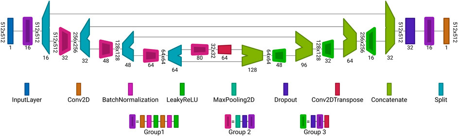
FIGURE 6. Proposed autoencoder architecture for reconstruction of data from noisy or blurred input. Each block is a set of layers. The values written vertically describe the dimension of the input for each layer, e.g., for noisy and blurred data r = 512, c = 512 and for the inverse modelling data r = 100, c = 100. The horizontally written values at the layers are the number of channels or number of filters. Group 1 is an combination of layers, consisting of: Conv2D, BatchNormlization, LeakyReLU, Conv2D, BatchNormlization and LeakyReLU layers. Group 2 is an extension of Group 1 where a MaxPooling2D and Dropout layer are placed before Group 1. Similar applies to Group 3, it consists of a Dropout layer followed by the layers from Group 1 and finalized by a Conv2DTranspose layer follows. The architecture was visualized with Net2Vis [55].

FIGURE 7

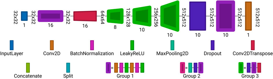
FIGURE 7. Autoencoder architecture used for reconstruction from undersampled observations. Each block is a set of layers. The layer labeling is the same as in Figure 6. Visualized with Net2Vis [55].

3 Results

In the following both machine learning methods will be applied to two tasks: (i) Reconstructing electrical excitation waves from noisy blurred and under sampled data (Section 3.1) and (ii) Predicting electrical excitation from mechanical contraction (Section 3.2).

3.1 Recovering Complex Spatio-Temporal Wave Patterns From Impaired Observations

To benchmark both reconstruction methods, using ESNs and CAEs, we use time series generated by the BOCF model introduced in Section 2.1.1. The same data were used for both methods, consisting of 5,002 samples in the training data set, 2,501 samples in the validation data set, and 2,497 samples in the test data set. The sampling time of all time series equalled $10\text{Δ}t=1$. We considered nine cases of noisy data (with different noise levels), ten cases of (differently) blurred data and seven examples of (spatially) undersampled time series.

For the implemention of the ESN we used the software package easyesn [56]. To determine the optimal ESN hyperparameters a grid search is performed as described in [18] using the training and validation subsets of the data. This search consists of two stages: first, for each combination of the local states’ hyperparameters σ and $\text{Δ}\sigma$ as listed in Table 2 a grid search is performed to find the optimal five hyperparameters of the ESN resulting in 37 sets of optimal hyperparameters. To make these grid searches more feasible, they were performed just for a single input patch (area covered by the stencil, see Figure 5) in the spatial center of the training set and thus not using the full spatial data.

TABLE 2

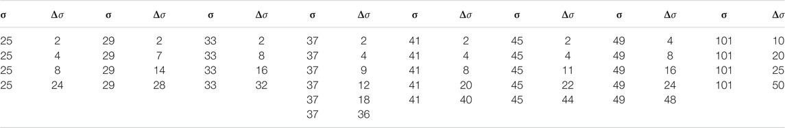
TABLE 2. The examined set of hyperparameters σ and $\text{Δ}\sigma$ for the local states.

TABLE 3

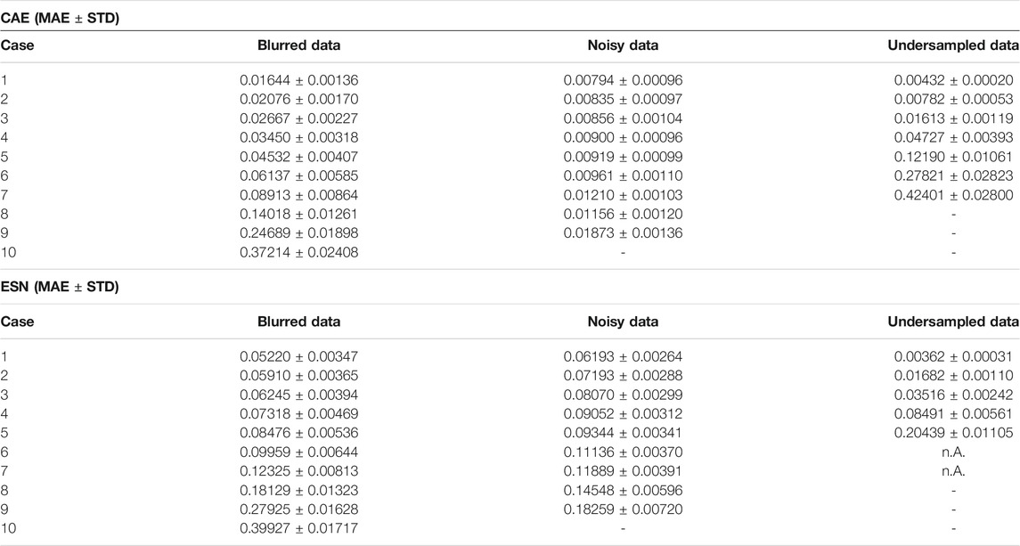
TABLE 3. Comparison of the MAE obtained when applying the CAE method and the ESN method to the test data set.

In the second stage, for each of the 37 sets of optimal hyperparameters determined before (for each combination of σ and $\text{Δ}\sigma$), an ESN is trained on a larger subset of the training data and not just on a single patch. Ideally, this step should be performed on the entire spatial domain of the training set, however, as we did not notice significant differences in the results when the ESNs were trained on a spatial subset of size $250\times 250$ to speed up the training process. Following the same methodology as in [18], for each pixel from this spatial subset a single ESN is trained and then the obtained output matrices ${\mathbf{W}}_{out}$ of these ESNs are averaged over all pixels. Compared to the procedure used in [18], the handling of boundary values has been changed. As for boundary pixels fewer adjacent pixels exist than for those inside, the creation of local states is obstructed, and boundary pixels require special treatment. In our previous work [18] individual ESNs have been trained for the boundary pixels using local states of lower dimensionality. In the following we use an alternative approach based on padding the boundary pixels by mirroring their values (motivated by the no-flux boundary conditions used). In this way, local states can be formally defined for boundary pixels in the same way as for inner pixels.

Next, the different optimal ESNs obtained for different stencils $\left(\sigma ,\text{Δ}\sigma \right)$ were evaluated by comparing their performance on the validation subset. In this way optimal values for σ and $\text{Δ}\sigma$ were selected by choosing the combination $\left(\sigma ,\text{Δ}\sigma \right)$ with the lowest ${\ell }_2$ difference between the prediction and ground truth on the validation set. This process yields an ESN whose hyperparameters and weights are optimized to yield minimal ${\ell }_2$ error. Finally, without training the network again on the entire training set, the optimal ESN found before is used to perform the prediction on the entire test set. As a pre-processing step, both the input and target data of the training, validation and test set are rescaled with min-max scaling, where the minimal and maximal value are determined over all pixels of the training set.

The CAE was trained using the ADAM optimizer [57], implemented with TensorFlow [58] in version 2.3, with early stopping when the validation loss has not improved at least by ${10}^{-6}$ for 20 epochs. The learning rate was reduced by a factor of 0.2 when the loss metric stopped improving at least by ${10}^{-5}$ for ten epochs. Dropout was set to be 0.05 in all cases. As loss function the mean absolute error (MAE) was chosen:

$\text{MAE}=\frac{1}{N}{\displaystyle \sum }_{i=1}^N|{\widehat{\mathbf{X}}}_i-{\mathbf{X}}_i^{\prime }|,(18)$

where N is the number of elements in the data set, ${\widehat{\mathbf{X}}}_i$ the network output, ${\mathbf{X}}_i^{\prime }$ desired ground-truth and $|.|$ stands for the absolute values.

3.1.1 Noisy Data

Figure 8 shows snapshots of the noisy input data, the corresponding ground truth, the outputs provided by the CAE and the ESN, respectively, and the absolute values of their prediction errors with respect to the ground truth.

FIGURE 8

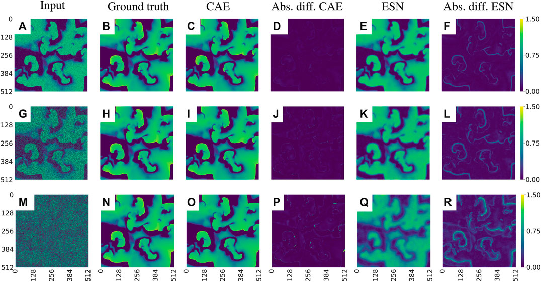
FIGURE 8. Exemplary visualization of the input and output for both networks for data with different noise levels p: (A)–(F)p = 0.1, (G)–(L)p = 0.5, and (M)–(R)p = 0.9. Comparing the absolute differences between the prediction and the ground truth [(D), (J), (P) for the CAE and (F), (L), (R) for the ESN] one can see that the CAE is less sensitive to noise. Note that the errors develop primarily on the fronts of the waves.

The evolution of the loss function during the training epochs is shown in Figure 9A. In all cases the error decreases and the training converges, but the duration of the training depends on the complexity of the case.

FIGURE 9

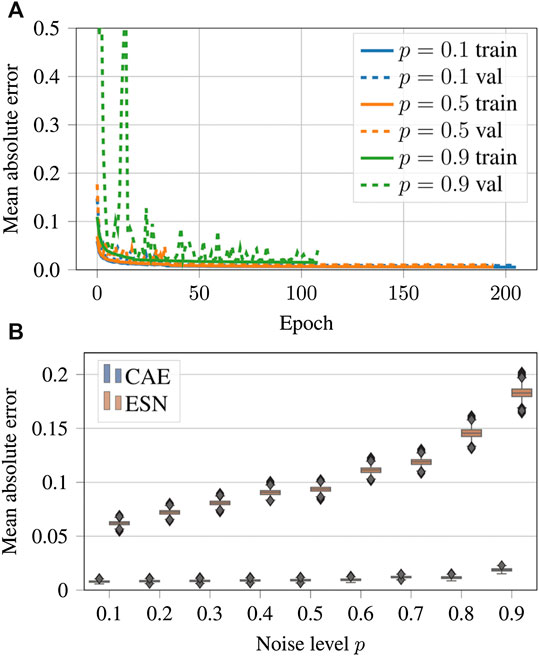
FIGURE 9. (A) Evolution of the loss function values over the epochs for noisy input data generated with noise levels $p=0.1$, $p=0.5$, and $p=0.9$ (compare Figure 8). It can be seen that the training always ran up to the point where early stopping, as defined in Section 3.1, terminated it. The solid lines are the values of the loss function during training on the training data, while the dotted lines are the values of the loss function obtained when the trained model is applied to the validation data. One epoch trained approximately 110 s on a GTX 1080 Ti. (B) Comparison between CAE and ESN performance with noisy input data showing boxplots of mean absolute errors (18) for different noise levels $p\in [0.1,0.2,\dots ,0.9]$. Each discrete value on the x-axis is assigned to the boxes of the CAE and ESN, where the ESN boxplots are colored in orange and the CNN boxplots are colored in blue. Note that for better visibility the CAE boxes and the ESN boxes a slightly shifted to the left and to the right, respectively. A tabular overview of the values can be found in Table 3).

Figures 9B shows a comparison of the performance of the CAE and the ESN for noisy data with nine different noise levels $p=0.1,\dots ,0.9$. While the mean absolute error of the CAE remains below 0.02, the reconstruction error of the ESN increases from 0.06 for $p=0.1$ to 0.18 for $p=0.9$, the associated ESN hyperparameter can be found in Table 4.

TABLE 4

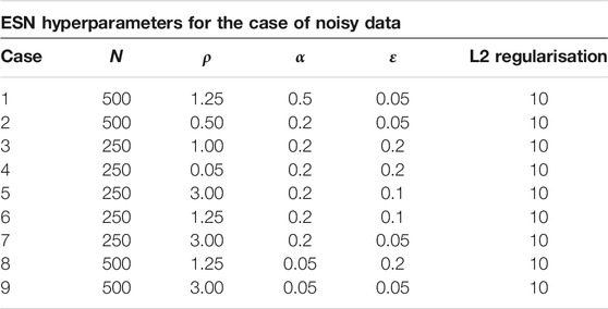
TABLE 4. Selected ESN hyperparameters for the case of noisy data.

3.1.2 Blurred Data

To evaluate the performance of CAE and ESN for recovering full resolution (ground truth) data from blurred observations we consider nine cases where the radius m of Fourier low-pass filtering ranges from $m=2$ to $m=18$ (in steps of 2). Figure 10 shows snapshots of reconstructions of the u-variable of the BOCF model using CAE and ESN with filter parameters $m=20$ (A-F), $m=14$ (G-L), and $m=8$ (M-R). Similar to Figure 8 the errors are largest at fronts of the excitation waves, but in contrast to noisy images the performances of CAE and ESN differ not much for blurred data. This observation is also confirmed by a systematic comparison of the mean absolute errors of both methods for different manhatten distances m given in Figure 11A. The errors decrease with m because the larger m the less blurred are the input data of the CAE or ESN (for hyperparameter see Table 5). Figure 11B shows the evolution of the loss function during training of the CAE.

TABLE 5

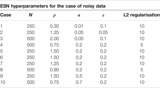
TABLE 5. Selected ESN hyperparameters for the case of blurred data.

FIGURE 10

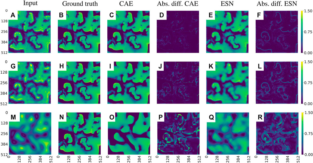
FIGURE 10. Exemplary visualization of the input and output for both networks, CAE and ESN, when recovering the original data from blurred measurements. (A)–(F) corresponds to case one, where $m=20$, (G)–(L) to case six with $m=14$ and (M)–(R) to seven, $m=8$. Comparing the absolute differences between the prediction and the ground truth [(D), (J), (P) for the CNN and (F), (L), (R) for the ESN] one recognizes that the CAE and ESN exhibit different patterns. The errors of the CAE are rather pointwise distributed at some locations [see (D), (J)] on the front while they are more evenly distributed when using ESNs (F), (L). This pattern is even more pronounced in (P) vs. (R).

FIGURE 11

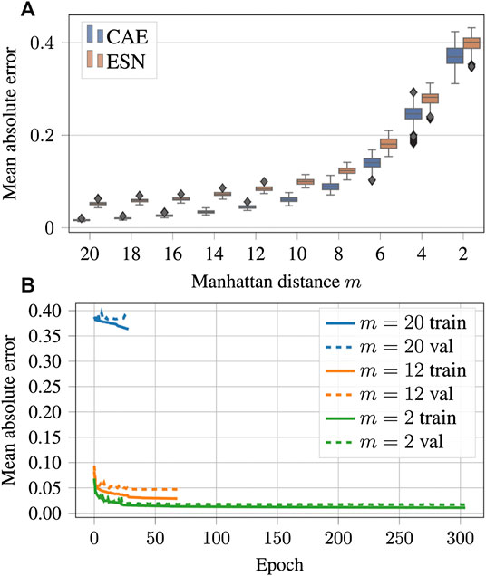
FIGURE 11. (A) Mean absolute errors of reconstructions using CAE or ESN from data blurred with different values of the low-pass filter parameter m. Like in Figure 9B boxes are horizontally shifted for better visibility. A tabular overview of the values can be found in Table 3. (B) Evolution of the loss function values over the training epochs for blurred data. Training was always terminated by reaching the early stopping criterion, defined in Section 3.1. One epoch trained approximately 108 s on a GTX 1080 Ti.

3.1.3 Undersampled Data

Figure 12 shows examples of data reconstructed from undersampled data. In total we considered seven cases of undersampling by $2^i$ pixels, where i ranges from $i=1$ to $i=7$. For $i=1$ input images have a resolution of $\mathbf{X}\in {\mathrm{ℝ}}^{256\times 256}$ and for $i=7$, $\mathbf{X}\in {\mathrm{ℝ}}^{4\times 4}$. In all cases the desired output (ground truth) ${\mathbf{X}}^{\prime }$ has a size of $512\times 512$ pixels. The used hyperparameter for the ESN can be found in Table 6). Figure 13B shows the evolution of the corresponding loss function.

FIGURE 12

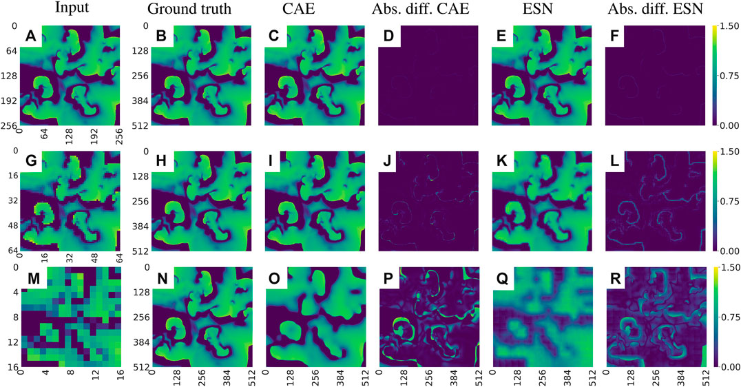
FIGURE 12. Exemplary visualization of the reconstruction of the u-field of the BOCF model from undersampled data. (A)–(F) corresponds to a sampling parameter $i=1$ resulting in $\mathbf{X}\in {\mathrm{ℝ}}^{256\times 256}$, (G)–(L) to case $i=3$, $\mathbf{X}\in {\mathrm{ℝ}}^{64\times 64}$ and (M)–(R) to $i=5$, $\mathbf{X}\in {\mathrm{ℝ}}^{16\times 16}$. With downsampling by a factor of $2^1$ reconstructions by both networks, CAEs and ESNs, are both very successful and the absolute differences shown in (D) and (F) are nearly zero. Similar to reconstructions from noisy or blurred data errors occur mainly at the fronts of the waves, and reconstruction errors of the CAE appear to be more localized compared to ESN results.

TABLE 6

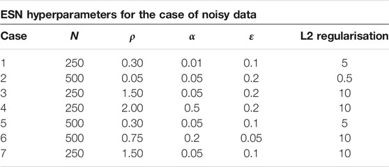
TABLE 6. Selected ESN hyperparameters for the case of undersampled data.

FIGURE 13

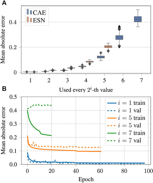
FIGURE 13. (A) Same as Figures 9B but for the case of the undersampled data. A tabular overview of the values can be found in Table 3. (B) Evolution of the loss function values over the epochs for undersampled input data.

3.2 Predicting Electrical Excitation From Mechanical Contraction

Echo state networks as well as convolutional autoencoders have been trained with time series generated by the electromechanical model introduced in Section 2.2 to predict the membrane voltage $u\left(x,t\right)$Eq. (4) from the local contraction $\text{Δ}A\left(x,t\right)$ given in Eq. (13). The sampling time of all time series equalled $6\text{Δ}t=0.48$. Since for periodically rotating spiral waves this cross-prediction task is quite straightforward we focus here on the much more demanding case of an example exhibiting spatio-temporal chaos (corresponding to atrial or ventricular fibrillation). Figure 14 shows at three instants of time snapshots of the observed contraction $\text{Δ}A$ (first column), the ground truth of the voltage u (second column), the prediction of the CAE $u_{\text{CAE}}$ and its absolute error $|u-u_{\text{CAE}}|$ (third and fourth column) and the prediction of the ESN $u_{\text{ESN}}$ and the corresponding absolute error $|u-u_{\text{ESN}}|$ (columns five and six, respectively). Both, the ESN and the CAE were trained and tested with the same spatio-temporal time series (lengths of training, validation and test sets are 15,000, 2000 and 2000 samples, respectively). Hyperparameters of the ESN are $N=600,\alpha =0.5,\rho =1.1,\mathit{ϵ}=0.05,\lambda =5\cdot {10}^{-3},\sigma =7$ and $\text{Δ}\sigma =1$. To make the ESN more robust normally distributed noise with zero mean and a variance of ${10}^{-4}$ was added to the arguments of the activation function.

FIGURE 14

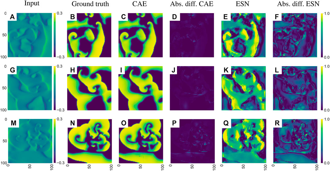
FIGURE 14. Exemplary visualization of the input and output for both networks for the inverse reconstruction of the membrane voltage uEq. (4) based on the mechanical deformation $\text{Δ}A$Eq. (13). (A)–(F) corresponds to $t=\mathrm{1,000}$, (G)–(L) to $t=\mathrm{1,500}$ and M-R to $t=\mathrm{2,000}$ of the test data set. The input is the mechanical deformation given by Eq. (13) caused by the electrical potential u from Eq. (4).

As illustrated in Figure 14 both networks can solve the inverse problem and reconstruct the electrical potential field u from Eq. (4). However, the reconstruction of the CAE is more precise, which is particularly noticeable at the edges of the reconstructed electrical potential field. Considering the median of the MAE over the entire test data the ESN approach achieves an error of $0.1963\pm 0.0260$ while the median error of the CAE equals $0.0164\pm 0.0028$.

4 Conclusion

Using synthetic data generated with conceptual models describing complex cardiac dynamics we have demonstrated possible applications of machine learning methods to complete and enhance experimental observations. It was shown that echo state networks as well as convolution autoencoders provide promising results, where the latter turned out to be the method of choice in terms of more faithful reconstructions. At this point, however, we would like to stress, that we didn’t try to fully optimize the algorithms employed. One could, for example, increase the size of the ESNs used or extend and refine the grid search of hyperparameters. Also with the CAE several options exist to improve the performance even more. Instead of the MAE in the loss function one could use an adaptive robust loss function [59] or the Jensen-Shannon divergence [19]. The weights of the CAE could be optimized with a stochastic gradient descend approach instead of the ADAM algorithm [57]. But we expect such modifications would show only minor improvements (if at all) [60, 61].

A comparison of the computing times with ESNs and CAEs is unfortunately not immediately possible. For the CAE the training time depends on the convergence, as illustrated in Figures 9A, 11B and 13B. In contrast to this, for ESNs training times depend strongly on the search for optical hyperparameters, especially the size of the reservoir, and this search is strongly dependent on the search space size and the number of parameters. For the task where electrical excitation is predicted from mechanical contraction our computations took 3,382 s on two Intel Xeon CPU E5-4620. While the CAE simulations have been run on GPUs the training and application of the ESN was on CPUs which makes a direct comparison difficult. Furthermore, the runtime of the programmes used is highly dependent on the libraries used and how well they have been adapted to special system architectures. In general we would estimate that in this work the effort to train and search hyperparameters for an ESN was a bit less demanding, in the sense of computational resources, compared to the training of the CAE. However, we would not consider the difference big enough to be an advantage for the ESN approach. Once trained both approaches need comparable execution times when applied to new data and executed on a CPU. In future work, using more realistic numerical simulations (and experimental data) such an optimization should be performed to achieve the best possible result for the intended medical application. Since here we used only data from conceptual models we refrained from fully optimizing the machine learning methods applied. The fact that already a straight-forward application of known algorithms and architectures provided very good results for the considered reconstruction tasks is very promising and encourages to address in future work extended tasks (including other variables, like calcium concentration, mechanical stress and strain, etc.) and reconstruction tasks with more realistic synthetic data (from 3D models, for example) combined with experimental measurements.

Data Availability Statement

The raw data supporting the conclusions of this article will be made available by the authors, without undue reservation. The source code will be available at https://gitlab.gwdg.de/sherzog3/reconstructing-cardiac-excitation-waves.git.

Author Contributions

SH performed the CAE simulations and RZ and JA did the ESN modelling. All authors designed the study, analyzed the results, and wrote the manuscript.

Funding

SH acknowledges funding by the International Max Planck Research Schools of Physics of Biological and Complex Systems. UP and SL acknowledge funding by the Max Planck Society, the German Center for Cardiovascular Research (DZHK) partner site Goettingen, and the SFB 1002 Modulatory Units in Heart Failure (Project C03).

Conflict of Interest

The authors declare that the research was conducted in the absence of any commercial or financial relationships that could be construed as a potential conflict of interest.

Acknowledgments

SH and UP thank Florentin Wörgötter and Thomas Lilienkamp for continuous support and inspiring scientific discussions.

Appendix 1: solution of the electro-mechanical dynamics

The differential equations from the extended Aliev-Panfilov model in Eqs. A1–A3 have been integrated using the forward Euler method $y_i^{t+\text{Δ}t}=y_i^t+\text{Δ}t\cdot f\left(y\right)+\mathrm{}\left(\text{Δ}{t}^2\right)$, in which y is a place holder for the model variables u, v and $T_a$; $f\left(y\right)$ represents the right-hand side of the respective equation. The diffusion tensor $\mathbf{D}$ in Equation (4) was set to a scalar constant D and the diffusion term was approximated with a nine-point stencil [60]

$\begin{array}{l}\nabla \left(\mathbf{D}\cdot \nabla u_{ij}\right)=D\cdot {\nabla }^2{u}_{ij}=\frac{D}{6h^2}(4u_{i+1,j}+4u_{i-1,j}+4u_{i,j+1}+4u_{i,j-1}+u_{i+1,j+1}+u_{i+1,j-1}+u_{i-1,j+1}+u_{i-1,j-1}-20u_{ij})+O(h^4)\end{array}(\mathrm{A1})$

where i, j are the indices of the grid points and h denotes the spacing constant between the cells.

For the excitation variable u in the electrical part of the simulation, no-flux boundary conditions have been used which were imposed by setting the two outermost cells to the same value, i.e., $u_{0,j}=u_{1,j}$. In the mechanical part of the simulation, numerical calculations were carried out according to the following scheme for each time step: (1) update of the position of the centre of mass $x_{cm}$, (2) calculation of all four points of attachment $q_i$ for each cell, (3) computing of forces from structural and axial springs for each particle $x_i$, (4) update of the positions of all particles using the Verlet method and (5) determine change of area for each cell. Here the Verlet method refers to the standard Verlet algorithm which is given as [61]

${\overrightarrow{x}}_i^{t+\text{Δ}t}=2{\overrightarrow{x}}_i^t-{\overrightarrow{x}}_i^{t-\text{Δ}t}+\frac{1}{m_i}{\overrightarrow{F}}_i^t\text{Δ}{t}^2+\mathrm{}\left(\text{Δ}{t}^4\right) ,(\mathrm{A2})$

with the total force ${\overrightarrow{F}}_i^t$ acting on the particle. Because the total force includes the damping term, it is convenient to rewrite Eq. A2 with ${\overrightarrow{F}}_i={\overrightarrow{f}}_i-\nu \frac{\text{d}{\overrightarrow{x}}_i}{\text{d}t}$ to

${\overrightarrow{x}}_i^{t+\text{Δ}t}=\frac{2{\overrightarrow{x}}_i^t-{\overrightarrow{x}}_i^{t-\text{Δ}t}\left(1-\frac{\nu }{2m_i}\text{Δ}t\right)+\frac{1}{m_i}{\overrightarrow{f}}_i^t\text{Δ}{t}^2}{1+\frac{\nu }{2m_i}\text{Δ}t}+\mathrm{}\left(\text{Δ}{t}^4\right) .(\mathrm{A3})$

A padding layer of ten electrically inactive cells was implemented outside the electrical grid to account for boundary effects in the mechanical network. In addition, the active stress variable $T_a$ from Eq. (6) of the last row of cells just at the edge of the simulation grid was mirrored to the two padding layers just outside the simulation grid which proved to dramatically reduce mechanical boundary effects. This is likely due to the fact that a proper contraction of an electrically active cell is not guaranteed if one of its sides is connected to an inactive cell. Lastly, the outermost padding cell’s positions were fixed to prevent the grid as a whole from moving away from its original position.

To improve numerical accuracy for each time step $\text{Δ}t$ of the electrical equations (Euler method) five time steps of size $\text{Δ}t/5$ were computed for the mechanical system (3). All computations have been performed on a spatial grid of 100 $\times$ 100 elements. The parameter values of the dynamical equations used are given in Table A1.

TABLE A1

TABLE A1. Parameters of the electro-mechanical model.

References

1. Gray, RA, Pertsov, AM, and Jalife, J. Spatial and temporal organization during cardiac fibrillation. Nature (1998). 392:75–8. doi:10.1038/32164

PubMed Abstract | CrossRef Full Text | Google Scholar

2. Davidenko, JM, Pertsov, AV, Salomonsz, R, Baxter, W, and Jalife, J. Stationary and drifting spiral waves of excitation in isolated cardiac muscle. Nature (1992). 355:349–51. doi:10.1038/355349a0

PubMed Abstract | CrossRef Full Text | Google Scholar

3. Witkowski, FX, Leon, LJ, Penkoske, PA, Giles, WR, Spano, ML, Ditto, WL, et al. Spatiotemporal evolution of ventricular fibrillation. Nature (1998). 392:72–82. doi:10.1038/32170

CrossRef Full Text | Google Scholar

4. Efimov, IR, Nikolski, VP, and Salama, G. Optical imaging of the heart. Circ Res (2004). 95:21–33. doi:10.1161/01.RES.0000130529.18016.35

PubMed Abstract | CrossRef Full Text | Google Scholar

5. Rosenzweig, S, Scholand, N, Holme, HCM, and Uecker, M. Cardiac and respiratory self-gating in radial mri using an adapted singular spectrum analysis (ssa-fary). IEEE Trans Med Imag (2020). 39:3029–3041.

CrossRef Full Text | Google Scholar

6. Otani, N, Luther, S, Singh, R, and Gilmour, R. Transmural ultrasound-based visualization of patterns of action potential wave propagation in cardiac tissue. Ann Biomed Eng (2010a). 38:3112–23.

PubMed Abstract | CrossRef Full Text | Google Scholar

7. Otani, N, Luther, S, Singh, R, and Gilmour, R. Methods and systems for functional imaging of cardiac tissueInternational Patent. London: World Intellectual Property Organization (2010b).

CrossRef Full Text | Google Scholar

8. Provost, J, Lee, WN, Fujikura, K, and Konofagou, EE. Imaging the electromechanical activity of the heart in vivo. Proc Natl Acad Sci USA (2011). 108:8565–70. doi:10.1073/pnas.1011688108

PubMed Abstract | CrossRef Full Text | Google Scholar

9. Bers, DM. Cardiac excitation-contraction coupling. Nature (2002). 415:198–205. doi:10.1038/415198a

PubMed Abstract | CrossRef Full Text | Google Scholar

10. Bourgeois, EB, Bachtel, AD, Huang, J, Walcott, GP, and Rogers, JM. Simultaneous optical mapping of transmembrane potential and wall motion in isolated, perfused whole hearts. J Biomed Optic (2011). 16:096020. doi:10.1117/1.3630115

CrossRef Full Text | Google Scholar

11. Zhang, H, Iijima, K, Huang, J, Walcott, GP, and Rogers, JM. Optical mapping of membrane potential and Epicardial deformation in beating hearts. Biophys J (2016). 111:438–51. doi:10.1016/j.bpj.2016.03.043

PubMed Abstract | CrossRef Full Text | Google Scholar

12. Christoph, J, Schröder-Schetelig, J, and Luther, S. Electromechanical optical mapping. Prog Biophys Mol Biol (2017). 130:150–69. doi:10.1016/j.pbiomolbio.2017.09.015

PubMed Abstract | CrossRef Full Text | Google Scholar

13. Christoph, J, Chebbok, M, Richter, C, Schroeder-Schetelig, J, Stein, S, Uzelac, I, et al. Electromechanical vortex filaments during cardiac fibrillation. Nature (2018). 555:667–72. doi:10.1038/nature26001

PubMed Abstract | CrossRef Full Text | Google Scholar

14. Berg, S, Luther, S, and Parlitz, U. Synchronization based system identification of an extended excitable system. Chaos: An Interdisciplinary Journal of Nonlinear Science (2011). 21:033104. doi:10.1063/1.3613921

CrossRef Full Text | Google Scholar

15. Lebert, J, and Christoph, J. Synchronization-based reconstruction of electromechanical wave dynamics in elastic excitable media. Chaos: An Interdisciplinary Journal of Nonlinear Science (2019). 29:093117. doi:10.1063/1.5101041

CrossRef Full Text | Google Scholar

16. Hoffman, MJ, LaVigne, NS, Scorse, ST, Fenton, FH, and Cherry, EM. Reconstructing three-dimensional reentrant cardiac electrical wave dynamics using data assimilation. Chaos Interdiscipl J Nonlinear Sci (2016). 26:013107. doi:10.1063/1.4940238

CrossRef Full Text | Google Scholar

17. Hoffman, MJ, and Cherry, EM. Sensitivity of a data-assimilation system for reconstructing three-dimensional cardiac electrical dynamics. Phil Trans Math Phys Eng Sci (2020). 378:20190388. doi:10.1098/rsta.2019.0388

CrossRef Full Text | Google Scholar

18. Zimmermann, RS, and Parlitz, U. Observing spatio-temporal dynamics of excitable media using reservoir computing. Chaos Interdiscipl J Nonlinear Sci (2018). 28:043118. doi:10.1063/1.5022276

CrossRef Full Text | Google Scholar

19. Herzog, S, Wörgötter, F, and Parlitz, U. Data-driven modeling and prediction of complex spatio-temporal dynamics in excitable media. Front Appl Math Stat (2018). 4:60. doi:10.3389/fams.2018.00060

CrossRef Full Text | Google Scholar

20. Herzog, S, Wörgötter, F, and Parlitz, U. Convolutional autoencoder and conditional random fields hybrid for predicting spatial-temporal chaos. Chaos (2019). 29:123116. doi:10.1063/1.5124926

PubMed Abstract | CrossRef Full Text | Google Scholar

21. Christoph, J, and Lebert, J. Inverse mechano-electrical reconstruction of cardiac excitation wave patterns from mechanical deformation using deep learning. Chaos (2020). 30:123134. doi:10.1063/5.0023751

CrossRef Full Text | Google Scholar

22. Bueno-Orovio, A, Cherry, EM, and Fenton, FH. Minimal model for human ventricular action potentials in tissue. J Theor Biol (2008). 253:544–60. doi:10.1016/j.jtbi.2008.03.029

PubMed Abstract | CrossRef Full Text | Google Scholar

23. Clayton, R, Bernus, O, Cherry, E, Dierckx, H, Fenton, F, Mirabella, L, et al. Mathematical and modelling foundations, models of cardiac tissue electrophysiology: progress, challenges and open questions Prog Biophys Mol Biol (2011). 104:22–48. doi:10.1016/j.pbiomolbio.2010.05.008

PubMed Abstract | CrossRef Full Text | Google Scholar

24. Ten Tusscher, K, Noble, D, Noble, P, and Panfilov, AV. A model for human ventricular tissue. Am J Physiol Heart Circ Physiol (2004). 286:H1573–H1589.

PubMed Abstract | CrossRef Full Text | Google Scholar

25. Strain, MC, and Greenside, HS. Size-dependent transition to high-dimensional chaotic dynamics in a two-dimensional excitable medium. Phys Rev Lett (1998). 80:2306–9. doi:10.1103/PhysRevLett.80.2306

CrossRef Full Text | Google Scholar

26. Lilienkamp, T, Christoph, J, and Parlitz, U. Features of chaotic transients in excitable media governed by spiral and scroll waves. Phys Rev Lett (2017). 119:054101.

PubMed Abstract | CrossRef Full Text | Google Scholar

27. Aliev, RR, and Panfilov, AV. A simple two-variable model of cardiac excitation. Chaos Solit Fractals (1996). 7:293–301. doi:10.1016/0960-0779(95)00089-5

CrossRef Full Text | Google Scholar

28. Nash, MP, and Panfilov, AV. Electromechanical model of excitable tissue to study reentrant cardiac arrhythmias. Prog Biophys Mol Biol (2004). 85:501–22. doi:10.1016/j.pbiomolbio.2004.01.016

PubMed Abstract | CrossRef Full Text | Google Scholar

29. Göktepe, S, and Kuhl, E. Electromechanics of the heart: a unified approach to the strongly coupled excitation–contraction problem. Comput Mech (2009). 45:227–43. doi:10.1007/s00466-009-0434-z

CrossRef Full Text | Google Scholar

30. Eriksson, TSE, Prassl, A, Plank, G, and Holzapfel, G. Influence of myocardial fiber/sheet orientations on left ventricular mechanical contraction. Math Mech Solid (2013). 18:592–606. doi:10.1177/1081286513485779

CrossRef Full Text | Google Scholar

31. Bourguignon, D, and Cani, MP. Controlling anisotropy in mass-spring systems. Eurographics. Vienna: Springer (2000). p. 113–23. doi:10.1007/978-3-7091-6344-3_9

CrossRef Full Text | Google Scholar

32. Jaeger, HGMD Report. The ‘echo state’ approach to analysing and training recurrent neural networks—with an erratum note. Kaiserslauten: German National Research Institute for Computer Science (2001). p. 43.

CrossRef Full Text | Google Scholar

33. Cheng, Z, Sun, H, Takeuchi, M, and Katto, J. Deep convolutional autoencoder-based lossy image compressionPicture Coding Symposium, PCS 2018—Proceedings. London: Institute of Electrical and Electronics Engineers Inc. (2018). p. 253–7. doi:10.1109/PCS.2018.8456308

CrossRef Full Text | Google Scholar

34. Lukoševičius, M. A practical guide to applying echo state networks. Lecture notes in computer science. Berlin: Springer (2012). p. 659–86. doi:10.1007/978-3-642-35289-8_36

CrossRef Full Text | Google Scholar

35. Lukoševičius, M, and Jaeger, H. Reservoir computing approaches to recurrent neural network training. Comput Sci Rev (2009). 3:127–49. doi:10.1016/j.cosrev.2009.03.005

CrossRef Full Text | Google Scholar

36. Yildiz, IB, Jaeger, H, and Kiebel, SJ. Re-visiting the echo state property. Neural Netw (2012). 35:1–9. doi:10.1016/j.neunet.2012.07.005

PubMed Abstract | CrossRef Full Text | Google Scholar

37. Jaeger, H, and Haas, H. Harnessing nonlinearity: predicting chaotic systems and saving energy in wireless communication. Science (2004). 304:78–80. doi:10.1126/science.1091277

PubMed Abstract | CrossRef Full Text | Google Scholar

38. Lu, Z, Pathak, J, Hunt, B, Girvan, M, Brockett, R, and Ott, E. Reservoir observers: model-free inference of unmeasured variables in chaotic systems. Chaos Interdiscipl J Nonlinear Sci (2017). 27:041102. doi:10.1063/1.4979665

CrossRef Full Text | Google Scholar

39. Carroll, TL, and Pecora, LM. Network structure effects in reservoir computers. Chaos Interdiscipl J Nonlinear Sci (2019). 29:083130. doi:10.1063/1.5097686

CrossRef Full Text | Google Scholar

40. Griffith, A, Pomerance, A, and Gauthier, DJ. Forecasting chaotic systems with very low connectivity reservoir computers. Chaos Interdiscipl J Nonlinear Sci (2019). 29:123108. doi:10.1063/1.5120710

CrossRef Full Text | Google Scholar

41. Thiede, LA, and Parlitz, U. Gradient based hyperparameter optimization in echo state networks. Neural Network (2019). 115:23–9. doi:10.1016/j.neunet.2019.02.001

PubMed Abstract | CrossRef Full Text | Google Scholar

42. Haluszczynski, A, Aumeier, J, Herteux, J, and Rth, C. Reducing network size and improving prediction stability of reservoir computing. Chaos Interdiscipl J Nonlinear Sci (2020). 30:063136. doi:10.1063/5.0006869

CrossRef Full Text | Google Scholar

43. Carroll, TL. Dimension of reservoir computers. Chaos Interdiscipl J Nonlinear Sci (2020). 30:013102. doi:10.1063/1.5128898

CrossRef Full Text | Google Scholar

44. Fan, H, Jiang, J, Zhang, C, Wang, X, and Lai, YC. Long-term prediction of chaotic systems with machine learning. Phys Rev Res (2020). 2:012080. doi:10.1103/PhysRevResearch.2.012080

CrossRef Full Text | Google Scholar

45. Parlitz, U, and Hornstein, A. Dynamical prediction of chaotic time series. Chaos Complex Lett (2005). 1:135–44.

CrossRef Full Text | Google Scholar

46. Lu, Z, Hunt, BR, and Ott, E. Attractor reconstruction by machine learning. Chaos Interdiscipl J Nonlinear Sci (2018). 28:061104. doi:10.1063/1.5039508

CrossRef Full Text | Google Scholar

47. Pathak, J, Hunt, B, Girvan, M, Lu, Z, and Ott, E. Model-free prediction of large spatiotemporally chaotic systems from data: a reservoir computing approach. Phys Rev Lett (2018). 120. doi:10.1103/physrevlett.120.024102

PubMed Abstract | CrossRef Full Text | Google Scholar

48. Parlitz, U, and Merkwirth, C. Prediction of spatiotemporal time series based on reconstructed local states. Phys Rev Lett (2000). 84:1890–3. doi:10.1103/physrevlett.84.1890

PubMed Abstract | CrossRef Full Text | Google Scholar

49. LeCun, Y, Boser, BE, Denker, JS, Henderson, D, Howard, RE, Hubbard, WE, et al. Handwritten digit recognition with a back-propagation network. In: DS Touretzky, editor. Advances in neural information processing systems, 2 Burlington, MA: Morgan-Kaufmann (1990). p. 396–404.

CrossRef Full Text | Google Scholar

50. Ioffe, S, and Szegedy, C. Batch normalization: accelerating deep network training by reducing internal covariate shift. Proc Int Conf Mach Learn (2015). 37:448456. doi:10.1609/aaai.v33i01.33011682

CrossRef Full Text | Google Scholar

51. Maas, AL, Hannun, AY, and Ng, AY. “Rectifier nonlinearities improve neural network acoustic models Speech and Language Processing.” In ICML workshop on deep learning for audio (2013). p. 3.

CrossRef Full Text | Google Scholar

52. Hahnloser, RH, Sarpeshkar, R, Mahowald, MA, Douglas, RJ, and Seung, HS. Digital selection and analogue amplification coexist in a cortex-inspired silicon circuit. Nature (2000). 405:947.

PubMed Abstract | CrossRef Full Text | Google Scholar

53. Srivastava, N, Hinton, G, Krizhevsky, A, Sutskever, I, and Salakhutdinov, R. Dropout: a simple way to prevent neural networks from overfitting. J Mach Learn Res (2014). 15:1929–58. doi:10.1109/iwcmc.2019.8766500

CrossRef Full Text | Google Scholar

54. Dumoulin, V, and Visin, F. A guide to convolution arithmetic for deep learning (2016). arXiv e-printsarXiv:1603.07285

CrossRef Full Text | Google Scholar

55. Bäuerle, A, and Ropinski, T. Net2vis: transforming deep convolutional networks into publication-ready visualizations (2019). arXiv preprint arXiv:1902.04394.

CrossRef Full Text | Google Scholar

56. Zimmermann, R, and Thiede, L. easyesn (2020). Available at: https://github.com/kalekiu/easyesn.

CrossRef Full Text | Google Scholar

57. Kingma, DP, and Ba, J. Adam: a method for stochastic optimization (2014). arXiv e-printsarXiv:1412.6980.

CrossRef Full Text | Google Scholar

58. Abadi, M, Agarwal, A, Barham, P, Brevdo, E, Chen, Z, Citro, C, et al. TensorFlow: large-scale machine learning on heterogeneous systems (2015). Software available from tensorflow.org.

CrossRef Full Text | Google Scholar

59. Barron, JT. A general and adaptive robust loss function. Berlin: Springer (2019).

CrossRef Full Text | Google Scholar

60. Rosser, JB. Nine-point difference solutions for poisson's equation. Comput Math Appl (1975). 1:351–60. doi:10.1016/0898-1221(75)90035-8

CrossRef Full Text | Google Scholar

61. Scherer, POJ. Computational physics: simulation of classical and quantum systems. Berlin: Springer (2010). p. 147.

CrossRef Full Text | Google Scholar

62. Chugh, SS, Havmoeller, R, Narayanan, K, Singh, D, Rienstra, M, Benjamin, EJ, et al. Worldwide epidemiology of atrial fibrillation: a Global Burden of Disease 2010 Study. Circulation (2014) 129:837–847. doi:10.1161/CIRCULATIONAHA.113.005119

CrossRef Full Text | Google Scholar

63. Wolf, PA, Dawber, TR, Thomas, HE, and Kannel, WB. Epidemiologic assessment of chronic atrial fibrillation and risk of stroke: the Framingham study. Neurology (1978) 28:973–977.

CrossRef Full Text | Google Scholar

64. Manolio, TA, Kronmal, RA, Burke, GL, O'Leary, DH, and Price, TR. Short-term predictors of incident stroke in older adults. The Cardiovascular Health Study. Stroke (1996) 27:1479–1486.

CrossRef Full Text | Google Scholar