Some New Solutions of Non Linear Evolution Equations With Mutable Coefficients

1 Introduction

NonLinear Evolution Equations (NLEEs) plays a significant role in the analysis of mathematical modeling and soliton theory. These NLEEs, which are primarily studied in mathematics and physics play an important role and character in various branches of science and technology, such as propagation of shallow water waves, population statistics physics, fluid dynamics, condensed matter physics, computational physics, and geophysics. NLEEs also appear and are very important in many fields such as wave mechanics, dissipation mechanics, dispersion in optics, reaction and convection equations. Over the past few decades, many compelling methodologies for extracting exact solutions of NLEEs have been formulated. However, it is more difficult to solve the NLEEs but, various methods have been tried for solving NLEEs, such as the Hirota’s bilinear operations [1] truncated Painleve expansion [2], inverse scattering transform [3], extended tanh-function method [4], F-expansion method [5], tanh-coth method [6], Jacobi-elliptic function expansion [7], homogenous balance method [8], sub ODE method [9], Rank analysis method [10], Extended and modified direct algebraic method [11], extended mapping method [12, 13] and Seadawy techniques to find solutions for some nonlinear partial differential equations [14] and many other ansatzes comprising exponential and hyperbolic functions are accurately used for the analytic analysis of NLEEs. Recently a few other well-known methods are used to extract explicit solutions of soliton equations, as example the adomionos decomposition method [15], Darboux transformation (DT) [16], Hirota technique [17] etc. In early 1990s, Wang et al. [18] familiarize a new formalism called extended $(\frac{G^{\prime }}{G})$-expansion method for a decisive treatment of NLEEs. After that further applications of this method have also been proclaimed [19, 20]. Therefore, further to expand the domain of applications of extended $(\frac{G^{\prime }}{G})$-expansion formalism, in this work we examine the nonlinear Sharma-Tasso-Olver with mutable coefficients (STO) [21, 22] equation exact solutions are attained which are in form of hyperbolic, trigonometric and rational functions. In works of literature, many times it appears as an evolution equation acquiring many symmetries. The extended $(\frac{G^{\prime }}{G})$-expansion formalism has also been applied to the Zakharov Kuznetsov (ZK) equation [23] and abundant exact solutions are derived which included the trigonometric, rational, and hyperbolic functions. First of all, we describe the method and applied it to two given equations, all different possible wave solutions are presented by their 3D plots and their corresponding contour plots. At the end of this article, discussion and conclusion are given in detail in the last section.

2 The Method and its Applications

In order to solve NLEEs, defined with two independent variables x and t, in this section we highlights the important points of the extended $(\frac{G^{\prime }}{G})$-expansion formalism. Suppose a NLEEs is of the form

$P(u,u_t,u_x,u_{tt},u_{xt},u_{xx},\dots )=0,(1)$

where u = u (x, t) and P is polynomial in u = u (x, t)

Point 1: Let us introduce the wave variable

$\xi =x-ct,(2)$

so that

$u(x,t)=u(\xi ).(3)$

This leads to NonLinear ordinary differential equation (NLODE) as

$P(u,u_{\xi },u_{\xi \xi },u_{\xi \xi \xi },\dots )=0,(4)$

where u_ξ denotes differentiation of u wrt ξ.

Integrating the ODE (4) many times with setting the constant of integration to be zero.

Point 2: The solution of Eq. 4 can be expressed by a polynomial in extended $(\frac{G^{\prime }}{G})$ i.e.

$u(\xi )={\delta }_m{(\frac{G^{\prime }}{G})}^m+{\delta }_{m-1}{(\frac{G^{\prime }}{G})}^{m-1}+\dots ‥=\sum _{i=-m}^{i=m}{\delta }_i{(\frac{G^{\prime }}{G})}^i,(5)$

where G = G(ξ) entertain following ODE of the form

$G^{\prime \prime }+\gamma G^{\prime }+\rho G=0,(6)$

where δ_m, δ_m−1, …,δ₀, γ and ρ are constants to be found out later and δ_m ≠ 0.

Point 3: Replacing Eq. 5 into Eq. 4 and using Eq. 6, and assembling all terms with the equal order of $(\frac{G^{\prime }}{G})$ together, and then equating each participating and the resulting polynomial to be zero yields a set of mathematical statement for δ_m, δ_m−1, …,δ₀, c, γ and ρ.

Point 4: Since the general solutions of Eq. 6 have been well known for us, then substituting δ_m, δ_m−1, …,δ₀ and c and the general solutions of Eq. 6 into Eq. 5 we obtain more solitary wave solutions of NLEEs Eq. 1.

With this detailed mathematical explanation of the extended $(\frac{G^{\prime }}{G})$-expansion formalism, we now try to solve the NLEEs of physical importance as discussed in previous section.

3 Sharma-Tasso-Olver Equation

Nonlinear Sharma-Tasso-Olver (STO) the mutable coefficients have discussed in many branches of mathematical physics, science and engineering. STO equation reads as [21].

$u_t+f(t){\left(u{u}_x+\frac{1}{3}{u}^3\right)}_x+g(t)u_{xxx}=0.(7)$

This equation contains both linear dispersive term u_xxx and the double nonlinear terms uu_x and u_t. Here the parameters f(t) ≠ 0, g(t) ≠ 0 and are both temporal variable. Using a transformation STO (7) with new variable reads

$u(x,t)=u(\xi ),\xi =x+\frac{w}{\zeta }{\int }_0^{t}g(t)dt.(8)$

provided f(t) and g(t) in Eq. 7 should hold the condition f(t) = 3g(t). Integration Eq. 7, shorten to

$\frac{w}{\zeta }{u}_{\xi }+u_{\xi \xi \xi }+3{\left(u{u}_{\xi }+\frac{1}{3}{u}^3\right)}_{\xi }.(9)$

Homogeneous balance between linear dispersive term u_ξξ and the double nonlinear terms u³ solution are as suggested by formalism, we find n = 1

$u(\xi )={\delta }_0+{\delta }_1(\frac{G^{\prime }}{G})+{\delta }_{-1}{(\frac{G^{\prime }}{G})}^{-1},(10)$

where δ₀, δ₁, δ₋₁ are constants. Replacing Eq. 10 with Eq. 6 into Eq. 7, accumulating the coefficients of $(\frac{G^{\prime }}{G})$ we attain a set of mathematical statement for δ₀, δ₁, δ₋₁, w and ζ and solving set of equation by mathematical software, we have.

Case (1)

${\delta }_{-1}=\rho ,{\delta }_0=0,\zeta =\zeta ,{\delta }_1=1,\gamma =-{\gamma }^2\zeta +4\zeta \rho ,(11)$

Case (2)

${\delta }_{-1}=0,{\delta }_0=\frac{\gamma }{2},\zeta =\zeta ,{\delta }_1=1,\gamma =-\frac{1}{4}{\gamma }^2\zeta +\zeta \rho ,(12)$

so as per the first conditions the Eq. 10 will give

$\begin{array}{ccc}\hfill & \hfill & u_1(\xi )=(\frac{G^{\prime }}{G})-\rho {(\frac{G^{\prime }}{G})}^{-1},\hfill \\ \hfill & \hfill & \xi =x+\frac{-{\gamma }^2\zeta +4\zeta \rho }{\zeta }{\int }_0^{t}g(t)dt.\hfill \end{array}(13)$

For the second case Eq. 10 will give

$\begin{array}{ccc}\hfill & \hfill & u_2(\xi )=\frac{\gamma }{2}+(\frac{G^{\prime }}{G}),\hfill \\ \hfill & \hfill & \xi =x+\frac{\frac{-{\gamma }^2}{4}\zeta +\zeta \rho }{\zeta }{\int }_0^{t}g(t)dt.\hfill \end{array}(14)$

with the aid of Eq. 6, solutions of Eqs 13,14 are the solitary wave solutions as trigonometric, rational and hyperbolic functions.

Solution of first kind (1): when $\sqrt{{\gamma }^2-4\rho }$ greater than 0

$\begin{array}{ccc}\hfill u_1(\xi )& =\hfill & \left[(\sqrt{{\gamma }^2-4\rho })\right.\hfill \\ \hfill & \hfill & \left.\left(\frac{A_1\sinh \left(\frac{1}{2}\sqrt{{\gamma }^2-4\rho }\right)\xi +A_2\cosh \left(\frac{1}{2}\sqrt{{\gamma }^2-4\rho }\right)\xi }{2A_1\cosh \left(\frac{1}{2}\sqrt{{\gamma }^2-4\rho }\right)\xi +2A_2\sinh \left(\frac{1}{2}\sqrt{{\gamma }^2-4\rho }\right)\xi }\right)-\frac{\gamma }{2}\right]\hfill \\ \hfill & \hfill & -\rho \left[(\sqrt{{\gamma }^2-4\rho })\right.\hfill \\ \hfill & \hfill & {\left.\left(\frac{A_1\sinh \left(\frac{1}{2}\sqrt{{\gamma }^2-4\rho }\right)\xi +A_2\cosh \left(\frac{1}{2}\sqrt{{\gamma }^2-4\rho }\right)\xi }{2A_1\cosh \left(\frac{1}{2}\sqrt{{\gamma }^2-4\rho }\right)\xi +2A_2\sinh \left(\frac{1}{2}\sqrt{{\gamma }^2-4\rho }\right)\xi }\right)-\frac{\gamma }{2}\right]}^{-1}.\hfill \end{array}(15)$

$\begin{array}{ccc}\hfill u_2(\xi )& =\hfill & \frac{\gamma }{2}+\left[(\sqrt{{\gamma }^2-4\rho })\right.\hfill \\ \hfill & \hfill & \left.\left(\frac{A_1\sinh \left(\frac{1}{2}\sqrt{{\gamma }^2-4\rho }\right)\xi +A_2\cosh \left(\frac{1}{2}\sqrt{{\gamma }^2-4\rho }\right)\xi }{2A_1\cosh \left(\frac{1}{2}\sqrt{{\gamma }^2-4\rho }\right)\xi +2A_2\sinh \left(\frac{1}{2}\sqrt{{\gamma }^2-4\rho }\right)\xi }\right)-\frac{\gamma }{2}\right].\hfill \end{array}(16)$

Solution of second kind (2): when $\sqrt{{\gamma }^2-4\rho }$ less than 0

$\begin{array}{ccc}\hfill u_1(\xi )& =\hfill & \left[(\sqrt{4\rho -{\gamma }^2})\right.\hfill \\ \hfill & \hfill & \left.-\left(\frac{A_1\sinh \left(\frac{1}{2}\sqrt{4\rho -{\gamma }^2}\right)\xi +A_2\cosh \left(\frac{1}{2}\sqrt{4\rho -{\gamma }^2}\right)\xi }{2A_1\cosh \left(\frac{1}{2}\sqrt{4\rho -{\gamma }^2}\right)\xi +2A_2\sinh \left(\frac{1}{2}\sqrt{4\rho -{\gamma }^2}\right)\xi }\right)-\frac{\gamma }{2}\right]\hfill \\ \hfill & \hfill & -\rho \left[(\sqrt{4\rho -{\gamma }^2})\right.\hfill \\ \hfill & \hfill & {\left.-\left(\frac{A_1\sinh \left(\frac{1}{2}\sqrt{4\rho -{\gamma }^2}\right)\xi +A_2\cosh \left(\frac{1}{2}\sqrt{4\rho -{\gamma }^2}\right)\xi }{2A_1\cosh \left(\frac{1}{2}\sqrt{4\rho -{\gamma }^2}\right)\xi +2A_2\sinh \left(\frac{1}{2}\sqrt{4\rho -{\gamma }^2}\right)\xi }\right)-\frac{\gamma }{2}\right]}^{-1}\hfill \end{array}(17)$

$\begin{array}{ccc}\hfill u_2(\xi )& =\hfill & \frac{\gamma }{2}+\left[(\sqrt{4\rho -{\gamma }^2})\right.\hfill \\ \hfill & \hfill & \left.\left(\frac{A_1\sinh \left(\frac{1}{2}\sqrt{4\rho -{\gamma }^2}\right)\xi +A_2\cosh \left(\frac{1}{2}\sqrt{4\rho -{\gamma }^2}\right)\xi }{2A_1\cosh \left(\frac{1}{2}\sqrt{4\rho -{\gamma }^2}\right)\xi +2A_2\sinh \left(\frac{1}{2}\sqrt{4\rho -{\gamma }^2}\right)\xi }\right)-\frac{\gamma }{2}\right]\hfill \end{array}(18)$

Solution of third kind (3): when $\sqrt{{\gamma }^2-4\rho }$ equal to 0

$\begin{array}{ccc}\hfill u_1(\xi )& =\hfill & \left[\frac{A_1}{A_1+A_2\xi }-\frac{\gamma }{2}\right]-\rho {\left[\frac{A_1}{A_1+A_2\xi }-\frac{\gamma }{2}\right]}^{-1},\hfill \\ \hfill u_2(\xi )& =\hfill & \frac{\gamma }{2}+{\left[\frac{A_1}{A_1+A_2\xi }-\frac{\gamma }{2}\right]}^{-1}.\hfill \end{array}(19)$

where A₁ and A₂ are integration constants. All different possible traveling wave solutions are presented by their 3D plots and their corresponding contour plots (right side figures) (Figure 1). For simplicity of the plot, we have taken all required vales of δ₀, δ₁, δ₋₁, ζ(t), A₁, and A₂ and plotted for only the first solution u₁(χ) only. Important results are discussed in concluding remarks.

FIGURE 1

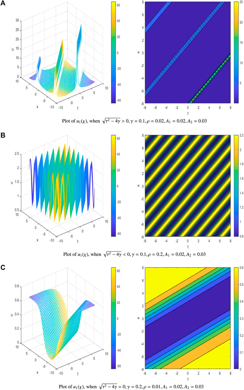
FIGURE 1. Traveling wave solution corresponding to the Sharma-Tasso-Olver (STO) equation. (A) Plot of u₁(χ), when $\sqrt{{\tau }^2-4\gamma }>0,\gamma =0.1,\rho =0.02,A_1=0.02,A_2=0.03$. (B) Plot of u₁(χ), when $\sqrt{{\tau }^2-4\gamma }<0,\gamma =0.1,\rho =0.2,A_1=0.02,A_2=0.03$. (C) Plot of u₁(χ), when $\sqrt{{\tau }^2-4\gamma }=0,\gamma =0.2,\rho =0.01,A_1=0.02,A_2=0.03$.

4 Generalized Zakharov Kuznetsov Equation

Generalized Zakharov Kuznetsov (ZK) equation with mutable coefficients describes wave features in plasma physics [23]. Particularly the ZK equation was a handful in for describing weakly nonlinear ion-acoustic waves in strongly magnetized lossless plasma in two dimensions. The ZK equation with dual power law nonlinearity is the main motivation of this work. The ZK equation reads as

$u_t\delta (t)u{u}_x+{\zeta }^2(t)u^2{u}_x+u_{xxx}+\theta (t)u_{xyy}=0.(20)$

where δ(t), ζ(t) and θ(t) are arbitrary function of t. For wave solutions for Eq. 20, use transformation

$u(x,t)=u(\xi ),\xi =kx+ly+{\int }_0^t\tau (t)dt.(21)$

where k, l are constants, τ(t) is an integrable function of t to be determined later. Substituting Eq. 21 into Eq. 20, we have

$\tau (t)u^{\prime }(\xi )+\delta (t)k{u}^{\prime }(\xi )u(\xi )+\zeta (t)k{u}^2(\xi )u^{\prime }(\xi )+[k^3+\theta (t)k{l}^2]u^{\prime \prime \prime }(\xi )=0.(22)$

where the prime denotes the differential with respect to x. Formalism suggests to introduce the anstaz

$u(\xi )={\delta }_m{\left(\frac{G^{\prime }}{G}\right)}^m+{\delta }_{m-1}{\left(\frac{G^{\prime }}{G}\right)}^{m-1}+\dots ‥=\sum _{i=-m}^{i=m}{\delta }_i{\left(\frac{G^{\prime }}{G}\right)}^i,(23)$

where δ_i are constants. Making the homogeneous balance between u′′′(ξ) and u²(ξ), u′(ξ) in Eq. 22, yields n = 1, so solution of Eq. 20 be as suggested by formalism

$u(\xi )={\delta }_0{\left(\frac{G^{\prime }}{G}\right)}^m+{\delta }_1{\left(\frac{G^{\prime }}{G}\right)}^1+{\delta }_{-1}{\left(\frac{G^{\prime }}{G}\right)}^{-1}.(24)$

Replacing Eq. 24 with Eq. 6 into Eq. 22, accumulating the coefficients of $(\frac{G^{\prime }}{G})$ for δ₀, δ₁, δ₋₁ and τ(t) and solving this system one can get.

Case (1)

$\begin{array}{ccc}\hfill & \hfill & {\delta }_0=\frac{{\delta }_1(\zeta (t){\delta }_1+6\theta (t)t^2\gamma +6k^2\gamma )}{12(k^2+\theta (t)t^2)},{\delta }_{-1}={\delta }_0,{\delta }_1={\delta }_1,\hfill \\ \hfill & \hfill & \eta =\eta ,k=k,\eta (t)=-\frac{6(k^2+\theta (t)t^2)}{{\delta }_1^2},\hfill \\ \hfill & \hfill & \tau (t)=\frac{k[12\theta (t)t^4{k}^2+96\theta (t)t^4\rho -\zeta {(t)}^2{\delta }_1^2]}{24(k^2+\theta (t)t^2)}\hfill \\ \hfill & \hfill & \frac{12\theta (t)t^4{k}^2+96\theta (t)t^4\rho -\zeta {(t)}^2{\delta }_1^2}{24(k^2+\theta (t)t^2)}.\hfill \end{array}(25)$

Case (2)

$\begin{array}{ccc}\hfill & \hfill & {\delta }_0=\frac{{\delta }_1(\zeta (t){\delta }_1+6\theta (t)l^2\gamma +6k^2\gamma )}{12(k^2+\theta (t)l^2)},{\delta }_{-1}=0,{\delta }_1={\delta }_1,\hfill \\ \hfill & \hfill & \eta (t)=-\frac{6(k^2+\theta (t)l^2)}{{\delta }_1^2},\hfill \\ \hfill & \hfill & \tau (t)=\frac{k\left\{24\theta (t)k^2{\gamma }^2{l}^2+12k^4{\gamma }^2+12\theta {(t)}^2{l}^4{\gamma }^2-96\theta (t)l^2\rho k^2\right.}{24(k^2+\theta (t)l^2)}\hfill \\ \hfill & \hfill & \frac{-48\theta {(t)}^2\rho l^4-{\zeta }^2(t){\delta }_1^2-48k^4\rho }{24(k^2+\theta (t)l^2)}.\hfill \end{array}(26)$

by using above two conditions solutions can be written as

$\begin{array}{ccc}\hfill & \hfill & u_1(\xi )=\frac{{\delta }_1(\zeta (t){\delta }_1+6\theta (t)t^2\gamma +6k^2\gamma )}{12(k^2+\theta (t)t^2)}+{\delta }_1{\left(\frac{G^{\prime }}{G}\right)}^1+{\delta }_{-1}{\left(\frac{G^{\prime }}{G}\right)}^{-1}\hfill \\ \hfill & \hfill & \xi =kx+ly\hfill \\ \hfill & \hfill & +{\int }_0^t\left[\frac{k(12\theta t^4{k}^2+96\theta t^4\rho -{\zeta }^2{\delta }_1^2)}{24(k^2+\theta (t)t^2)}\right]dt\hfill \\ \hfill & \hfill & +{\int }_0^t\left[\frac{k(12k^4{\gamma }^2+96k^4\rho +24\theta t^2{\gamma }^2{k}^2+192\theta t^2\rho k^2)}{24(k^2+\theta (t)t^2)}\right]dt\hfill \end{array}$

similarly we have

$\begin{array}{ccc}\hfill & \hfill & u_1(\xi )=\frac{{\delta }_1(\zeta (t){\delta }_1+6\theta (t)t^2\gamma +6k^2\gamma )}{12(k^2+\theta (t)l^2)}+{\delta }_1{\left(\frac{G^{\prime }}{G}\right)}^1+{\delta }_{-1}{\left(\frac{G^{\prime }}{G}\right)}^{-1}\hfill \\ \hfill & \hfill & \xi =kx+ly\hfill \\ \hfill & \hfill & +{\int }_0^t\left[\frac{k\{24\theta k^2{\gamma }^2{l}^2+12k^4{\gamma }^2+12{\theta }^2{l}^4{\gamma }^2\}}{24(k^2+\theta (t)l^2)}\right]dt\hfill \\ \hfill & \hfill & +{\int }_0^t\left[\frac{k\{96\theta l^2\rho k^2-48{\theta }^2\rho l^4-{\zeta }^2{\delta }_1^2-48k^4\rho \}}{24(k^2+\theta (t)l^2)}\right]dt\hfill \end{array}$

with Eq. 26 and Eq. 6, we have exponential and hyperbolic and rational functions types of solitary wave solutions for ZK equation with mutable coefficients Eq. 20 as:

Solution of first kind (1): when $\sqrt{{\gamma }^2-4\rho }>0$

$\begin{array}{ccc}\hfill u_1(\xi )& =\hfill & \left[(\sqrt{{\gamma }^2-4\rho })\right.\hfill \\ \hfill & \hfill & \left.\left(\frac{A_1\sinh \left(\frac{1}{2}\sqrt{{\gamma }^2-4\rho }\right)\xi +A_2\cosh \left(\frac{1}{2}\sqrt{{\gamma }^2-4\rho }\right)\xi }{2A_1\cosh \left(\frac{1}{2}\sqrt{{\gamma }^2-4\rho }\right)\xi +2A_2\sinh \left(\frac{1}{2}\sqrt{{\gamma }^2-4\rho }\right)\xi }\right)-\frac{\gamma }{2}\right]\hfill \\ \hfill & \hfill & +\frac{{\delta }_1(\zeta (t){\delta }_1+6\theta (t)t^2\gamma +6k^2\gamma )}{12(k^2+\theta (t)l^2)}+{\delta }_1\left[(\sqrt{{\gamma }^2-4\rho })\right.\hfill \\ \hfill & \hfill & {\left.\left(\frac{A_1\sinh \left(\frac{1}{2}\sqrt{{\gamma }^2-4\rho }\right)\xi +A_2\cosh \left(\frac{1}{2}\sqrt{{\gamma }^2-4\rho }\right)\xi }{2A_1\cosh \left(\frac{1}{2}\sqrt{{\gamma }^2-4\rho }\right)\xi +2A_2\sinh \left(\frac{1}{2}\sqrt{{\gamma }^2-4\rho }\right)\xi }\right)-\frac{\gamma }{2}\right]}^{-1}.\hfill \end{array}(27)$

$\begin{array}{ccc}\hfill u_2(\xi )& =\hfill & {\delta }_1\left[(\sqrt{{\gamma }^2-4\rho })\right.\hfill \\ \hfill & \hfill & \left.\left(\frac{A_1\sinh \left(\frac{1}{2}\sqrt{{\gamma }^2-4\rho }\right)\xi +A_2\cosh \left(\frac{1}{2}\sqrt{{\gamma }^2-4\rho }\right)\xi }{2A_1\cosh \left(\frac{1}{2}\sqrt{{\gamma }^2-4\rho }\right)\xi +2A_2\sinh \left(\frac{1}{2}\sqrt{{\gamma }^2-4\rho }\right)\xi }\right)-\frac{\gamma }{2}\right]\hfill \\ \hfill & \hfill & +\frac{{\delta }_1(\zeta (t){\delta }_1+6\theta (t)t^2\gamma +6k^2\gamma )}{12(k^2+\theta (t)l^2)}.\hfill \end{array}(28)$

Second kind (2): when $\sqrt{{\gamma }^2-4\rho }<0$

$\begin{array}{ccc}\hfill u_1(\xi )& =\hfill & {\delta }_1\left[(\sqrt{4\rho -{\gamma }^2})\right.\hfill \\ \hfill & \hfill & \left.-\left(\frac{A_1\sinh \left(\frac{1}{2}\sqrt{4\rho -{\gamma }^2}\right)\xi +A_2\cosh \left(\frac{1}{2}\sqrt{4\rho -{\gamma }^2}\right)\xi }{2A_1\cosh \left(\frac{1}{2}\sqrt{4\rho -{\gamma }^2}\right)\xi +2A_2\sinh \left(\frac{1}{2}\sqrt{4\rho -{\gamma }^2}\right)\xi }\right)-\frac{\gamma }{2}\right]\hfill \\ \hfill & \hfill & +\frac{{\delta }_1(\zeta (t){\delta }_1+6\theta (t)t^2\gamma +6k^2\gamma )}{12(k^2+\theta (t)l^2)}+{\delta }_1\left[(\sqrt{4\rho -{\gamma }^2})\right.\hfill \\ \hfill & \hfill & {\left.-\left(\frac{A_1\sinh \left(\frac{1}{2}\sqrt{4\rho -{\gamma }^2}\right)\xi +A_2\cosh \left(\frac{1}{2}\sqrt{4\rho -{\gamma }^2}\right)\xi }{2A_1\cosh \left(\frac{1}{2}\sqrt{4\rho -{\gamma }^2}\right)\xi +2A_2\sinh \left(\frac{1}{2}\sqrt{4\rho -{\gamma }^2}\right)\xi }\right)-\frac{\gamma }{2}\right]}^{-1}.\hfill \end{array}(29)$

$\begin{array}{ccc}\hfill u_2(\xi )& =\hfill & {\delta }_1\left[(\sqrt{4\rho -{\gamma }^2})\right.\hfill \\ \hfill & \hfill & \left.\left(\frac{A_1\sinh \left(\frac{1}{2}\sqrt{4\rho -{\gamma }^2}\right)\xi +A_2\cosh \left(\frac{1}{2}\sqrt{4\rho -{\gamma }^2}\right)\xi }{2A_1\cosh \left(\frac{1}{2}\sqrt{4\rho -{\gamma }^2}\right)\xi +2A_2\sinh \left(\frac{1}{2}\sqrt{4\rho -{\gamma }^2}\right)\xi }\right)-\frac{\gamma }{2}\right]\hfill \\ \hfill & \hfill & +\frac{{\delta }_1(\zeta (t){\delta }_1+6\theta (t)t^2\gamma +6k^2\gamma )}{12(k^2+\theta (t)l^2)}.\hfill \end{array}(30)$

Third kind (3): when $\sqrt{{\gamma }^2-4\rho }=0$

$\begin{array}{ccc}\hfill u_1(\xi )& =\hfill & {\delta }_1\left[\frac{A_1}{A_1+A_2\xi }-\frac{\gamma }{2}\right]+\frac{{\delta }_1\{\zeta (t){\delta }_1+6\theta (t)t^2\gamma +6k^2\gamma \}}{12(k^2+\theta (t)l^2)}\hfill \\ \hfill & \hfill & +{\delta }_1{\left[\frac{A_1}{A_1+A_2\xi }-\frac{\gamma }{2}\right]}^{-1},\hfill \end{array}(31)$

$u_2(\xi )={\delta }_1+{\left[\frac{A_1}{A_1+A_2\xi }-\frac{\gamma }{2}\right]}^{-1}+\frac{{\delta }_1\{\zeta (t){\delta }_1+6\theta (t)t^2\gamma +6k^2\gamma \}}{12(k^2+\theta (t)l^2)}.(32)$

where A₁ and A₂ are integration constants. As results, many exact solitary wave solutions of the form hyperbolic, trigonometric and rational functions are obtained (Figure 2). We have taken all required vales of δ₀, δ₁, δ₋₁, ρ, ζ(t), θ(t) k, l, A₁, A₂ and τ(t) and plotted for only the first solution u₁(χ) only.

FIGURE 2

FIGURE 2. Traveling wave solution corresponding to the Zakharov Kuznetsov equation (ZK) equation. (A) Plot of u₁(χ), when $\sqrt{{\tau }^2-4\gamma }>0,\gamma =0.1,\rho =0.02,A_1=0.02,A_2=0.03$. (B) Plot of u₁(χ), when $\sqrt{{\tau }^2-4\gamma }<0,\gamma =0.1,\rho =0.2,A_1=0.02,A_2=0.03$. (C) Plot of u₁(χ), when $\sqrt{{\tau }^2-4\gamma }=0,\gamma =0.2,\rho =0.01,A_1=0.02,A_2=0.03$.

5 Conclusion

Finally, it is worthwhile to mention these hyperbolic, trigonometric and rational function solutions are difficult to obtain by the methods mentioned in the introduction. The general solitary wave solutions can give soliton or periodic solutions under different parametric restrictions. These results mean that there are rich solitary wave patterns for the STO and ZK equation. To the best of our knowledge concern, this paper reports the aforementioned new solutions by this novel method. To our knowledge our solutions Eq. 15 and Eq. 17 of Eqs 19,27,29 of Eq. 32 are all new and not reported in literature. It is interesting to note that from the general results, one can easily recover solutions that are obtained from other methods. If we take the concrete parameters in a real model, we can give the corresponding representation of the solution. Comparing this work with the work in [6] where the tanh method were used, we find that the proposed method in this work presents more kink and solitons solutions compared to the work in [6]. Therefore, it is rather convenient for practice. We also presented three-dimensional plots and their corresponding contour plots of some of the solutions. This is direct and the concise method can further be used to explore more applications.

Data Availability Statement

The raw data supporting the conclusion of this article will be made available by the authors, without undue reservation.

Author Contributions

The author confirms being the sole contributor of this work and has approved it for publication.

Conflict of Interest

The author declares that the research was conducted in the absence of any commercial or financial relationships that could be construed as a potential conflict of interest.

Publisher’s Note

All claims expressed in this article are solely those of the authors and do not necessarily represent those of their affiliated organizations, or those of the publisher, the editors and the reviewers. Any product that may be evaluated in this article, or claim that may be made by its manufacturer, is not guaranteed or endorsed by the publisher.

References

1. Hirota, R. The Direct Method in Soliton Theory. Cambridge: Cambridge University Press (2004).

Google Scholar

2. Lou, SY, Wu, B, and Zhang, SL. Painlev Analysis and Special Solutions of Generalized Broer-Kaup Equations. Phys Lett A (2002) 300(1):4048. doi:10.1016/S0375-9601(02)00688-6

CrossRef Full Text | Google Scholar

3. Ablowitz, MJ, and Clarkson, PA. Soliton, Nonlinear Evolution Equations and Inverse Scattering. New York: Cambridge University Press (1991).

Google Scholar

4. Fan, E. Extended Tanh-Function Method and its Applications to Nonlinear Equations. Phys Lett A (2000) 277:212–8. doi:10.1016/s0375-9601(00)00725-8

CrossRef Full Text | Google Scholar

5. Yan, CT. A Simple Transformation for Nonlinear Waves. Phys Lett A (1995) 224:77–84. doi:10.1016/S0375-9601(96)00770-0

CrossRef Full Text | Google Scholar

6. Wazwaz, AM. The Tanh-Coth Method for Solitons and Kink Solutions for Nonlinear Parabolic Equations. Appl Math Comput (1997) 188:1467–75. doi:10.1016/j.amc.2006.11.013

CrossRef Full Text | Google Scholar

7. Fu, ZT, Liu, SK, Liu, SD, and Zhao, Q. Jacobi Elliptic Function Expansion Method and Periodic Wave Solutions of Nonlinear Wave Equations. Phys Lett A (2001) 289:69–74. doi:10.1016/S0375-9601(01)00580-1

CrossRef Full Text | Google Scholar

8. Ablowitz, MJ, and Clarkson, PA. Solitons, Non-linear Equations and Inverse Scattering Transform. Cambridge: Cambridge University Press (1991).

Google Scholar

9. Arshad, M, Seadawy, AR, and Lu, D. Modulation Stability and Optical Soliton Solutions of Nonlinear Schrödinger Equation with Higher Order Dispersion and Nonlinear Terms and its Applications. Superlattices and Microstructures (2017) 112:422–34. doi:10.1016/j.spmi.2017.09.054

CrossRef Full Text | Google Scholar

10. Yel, G, Baskonus, HM, and Gao, W. New Dark-Bright Soliton in the Shallow Water Wave Model. AIMS Math (2020) 5(4):40274044. doi:10.3934/math.2020259

CrossRef Full Text | Google Scholar

11. Seadawy, AR, and El-Rashidy, K. Dispersive Solitary Wave Solutions of Kadomtsev-Petviashvili and Modified Kadomtsev-Petviashvili Dynamical Equations in Unmagnetized Dust Plasma. Results Phys (2018) 8:1216–22. doi:10.1016/j.rinp.2018.01.053

CrossRef Full Text | Google Scholar

12. Seadawy, AR, Ali, A, and Albarakati, WA. Analytical Wave Solutions of the (2 + 1)-dimensional First Integro-Differential Kadomtsev-Petviashivili Hierarchy Equation by Using Modified Mathematical Methods. Results Phys (2019) 15:102775. doi:10.1016/j.rinp.2019.102775

CrossRef Full Text | Google Scholar

13. Helal, MA, Seadawy, AR, and Zekry, MH. Stability Analysis of Solitary Wave Solutions for the Fourth-Order Nonlinear Boussinesq Water Wave Equation. Appl Math Comput (2014) 232:1094–103. doi:10.1016/j.amc.2014.01.066

CrossRef Full Text | Google Scholar

14. Baskonus, HM. New Acoustic Wave Behaviors to the DaveyStewartson Equation with Power-Law Nonlinearity Arising in Fluid Dynamics. Nonlinear Dyn (2016) 86(1):177183. doi:10.1007/s11071-016-2880-4

CrossRef Full Text | Google Scholar

15. Iqbal, M, Seadawy, AR, Khalil, OH, and Lu, D. Propagation of Long Internal Waves in Density Stratified Ocean for the (2+1)-dimensional Nonlinear Nizhnik-Novikov-Vesselov Dynamical Equation. Results Phys (2020) 16:102838. doi:10.1016/j.rinp.2019.102838

CrossRef Full Text | Google Scholar

16. Tong, L, Wang, S, and Zhang, S. A Generalized (G′/G)- Expansion Method for the mKdv Equation with Variable Coefficients. Phys Lett A (2008) 372:2254. doi:10.1016/j.physleta.2007.11.026

CrossRef Full Text | Google Scholar

17. Gulnur, Y, Carlo, C, Haci, MB, and Wei, G. DarkBright to the Hirota-Maccari System. J Comput Nonlinear Dynam (2021) 16(6):061005. doi:10.1115/1.4050677

CrossRef Full Text | Google Scholar

18. Wang, M. Exact Solutions for a Compound Kdv-Burgers Equation. Phys Lett A (1996) 213:279–87. doi:10.1016/0375-9601(96)00103-x

CrossRef Full Text | Google Scholar

19. Li, X, Wang, M, and Zhang, J. The (G′/G)-expansion Method and Traveling Wave Solutions of Nonlinear Evolution Equations in Mathematical Physics. Phys Lett A (2008) 372:417. doi:10.1016/j.physleta.2007.07.051

CrossRef Full Text | Google Scholar

20. Wang, M. Solitary Wave Solutions for Variant Boussinesq Equations. Phys Lett A (1995) 199:169–72. doi:10.1016/0375-9601(95)00092-h

CrossRef Full Text | Google Scholar

21. Sharma, AS. Connection between Wave Envelope and Explicit Solution of a Nonlinear Dispersive Equation. Rep IPP (1977) 158:1.

Google Scholar

22. Olver, PJ. Evolution Equations Possessing Infinitely many Symmetries. J Math.Phys (1977) 18:12121215. doi:10.1063/1.523393

CrossRef Full Text | Google Scholar

23. Kuznetsov, EA, and Zakharov, VE. On Three-Dimensional Solitons. Sov. Phys. JETP (1974) 39:285288.

Google Scholar