A General Framework for Spatio-Temporal Modeling of Epidemics With Multiple Epicenters: Application to an Aerially Dispersed Plant Pathogen

1 Introduction

Epidemics caused by invasive pathogens can be managed through several approaches that include quarantine, containment, eradication programs, and chemical control measures. Understanding the risk of disease invasion is vital in facilitating the planning of disease control, prediction, prevention of epidemics, and development of mitigation policies [1]. These needs are particularly acute for fecund organisms capable of long-distance dispersal that are not spatially restricted. Dispersal is a fundamental process with many implications for invasion ecology. The characteristics and frequency of long-distance dispersal may influence processes such as spatial distribution of an organism, gene flow between populations, and invasiveness [2–6]. Dispersal characteristics of a pathogen are also central to formulating sound policies for mitigation of ensuing epidemics, such as predicting the first appearance of disease and timing of intervention efforts [5].

Diverse disease organisms may generate patterns of spread due to long-distance dispersal that can be explained by similar models provided that inoculum moves over long distances [7, 8]. Plant disease epidemics, therefore, are excellent model systems for understanding dispersal and its determinants due to the annual occurrence of epidemics and experimental tractability of these systems. One such disease example is cucurbit downy mildew, caused by the oomycete Pseudoperonospora cubensis. Cucurbit downy mildew is a major concern for growers in the eastern U.S. due to its ability to cause substantial economic losses. For example, in 2004 alone, the epidemic on cucumber resulted in $16 million USD economic loss [9]. In the U.S. and central Europe, the disease exhibits annual recolonization and extinction cycles, generating annual disease invasions at the continental scale because P. cubensis is aerially dispersed and sporangia can be transported over long distances [10, 11]. Additionally, P. cubensis is an obligate parasite that must overwinter on living host tissue. In the U.S., this is thought to restrict overwintering under natural conditions to frost-free areas below approximately 30-degree latitude [12, 13]. Historical data on the occurrence of the disease is available from standardized sentinel plots deployed as part of the Cucurbit Downy Mildew ipmPIPE program [11]. Furthermore, the disease is economically important and can result in complete crop loss in the absence of adequate control measures [13, 14]. Successful management also requires that control measures be implemented just before or at the first detection of the disease in a field or region.

Simple predictive models with analytical solutions have been used to analyze disease spread in plant epidemics when mechanistic models do not exist. We consider phenomenological models with empirical support in plant disease epidemiology as starting points for our framework. We focus on widely used models for both the temporal and spatial behavior of pathosystems driven by aerial dispersal. Although the models we present are descriptive and not mechanistic, we emphasize that the models are predictive of epidemic spread in space and time, even with sparse data sets. In what follows we provide a brief introduction to these common phenomenological models; the reader may find this introduction provides useful context, but may also opt to skip ahead, as the exposition of our framework beginning in Section 2-1 is sufficiently detailed to stand alone.

Infection of cucurbits by P. cubensis results in epidemics where inoculum is produced by plants previously infected during the same epidemic in that season. In plant disease epidemiology, such epidemics are termed polycyclic and the logistic model is one of the simplest in a class of models that are used to approximate the behavior of these epidemics over time [15]. The logistic model assumes that the rate of change (over time) of the disease intensity y at a site is proportional to the product of the disease intensity y and the healthy intensity 1 − y at that site,

$\frac{dy}{dt}=ay(1-y)(1)$

where a is the rate of disease progression. The observed disease intensity y for an individual site that gets infected during an epidemic is represented by the fraction Y/N, where Y represents the disease in absolute units (such as the number of lesions, infected leaves, or plants) at that site, and N represents the total number of individuals or plant area that can possibly be infected at that site. The value of y is bounded between 0 and 1, inclusively. For an epidemic to occur, there must be contact between inoculum and disease-free individuals. The latter is incorporated into the model by the expression 1 − y. Production and dispersal of inoculum from infected individuals, infection of healthy individuals, and subsequent production of new inoculum by the newly diseased individuals are incorporated into the model by the rate parameter a [15]. This model framework is widely used in plant disease epidemiology to describe diverse pathosystems [15].

Pathogens exhibiting long-distance dispersal result in epidemics with accelerating velocity over time that are often difficult to control [5]; inoculum of such pathogens arises from an initial disease focus (or multiple foci) and travels long distances where it may cause disease far from the initial focus. The long-distance spread of disease generates a spatial dispersal gradient relative to the focus–the rate of decrease in inoculum density with distance from a source [16]. For aerially dispersed pathogens, wind is the main dispersal mechanism of inoculum. Epidemics driven by aerial dispersal exhibit wave-like behavior in which spatial dispersal at any given time can be accurately approximated by a power-law [1]. The power-law model is of the form

$\frac{dy}{dr}=\frac{-by}{r}(2)$

or

$\frac{dy}{dr}=\frac{-by}{r+\lambda }(3)$

where r = r(t) denotes the maximum distance of the disease front from the epicenter (the radius of the disease spread) at time t, y = y(t) denotes the disease intensity at the disease front, b is the spread parameter (unitless), and λ is an offset parameter incorporated into the model to permit calculations at r = 0. The power-law model only approximates epidemic behavior well on certain spatial scales; when y is large and r is small. The above two versions of the power-law model can produce extreme values for $\frac{dy}{dr}$, which are inconsistent with realistic dispersal behaviors, if the values of b and λ are chosen in such a way that the model approximates the dispersal behavior at locations farther from the source position very well. In addition, the model implies an upper limit to disease intensity at any given location. A simple modification overcomes these limitations:

$\frac{dy}{dr}=\frac{-by(1-y)}{r+\lambda }(4)$

Eq. 4 is known as a power-logistic model [15]. This power-logistic model is consistent with empirical observations for disease spread at multiple spatial scales [15] unlike the models described in Eq. 2, and Eq. 3.

Disease epidemics are dynamic population processes occurring in both time and space; the above phenomenological models can jointly approximate such spatiotemporal dynamics. For sparse observational data, it is often of interest to describe the epidemic wavefront–the point(s) which is the farthest from the position of the source among all points where the disease is present. To this end, fix a reference point (not necessarily the source of the epidemic), and let r(t) (resp. y(t)) denote the signed distance of the wavefront from the reference point (resp. disease intensity at the wavefront) at time t. Here and later, the signed distance of $(u,v)\in {\mathbb{R}}^2$ from $(w,z)\in {\mathbb{R}}^2$ is

$d((w,z),(u,v))\left\{\begin{array}{cc}+\sqrt{{(u-w)}^2+{(v-z)}^2}\hfill & \text{\hspace{0.17em}if\hspace{0.17em}either}u>w,oru=w\text{and}v>z\hfill \\ -\sqrt{{(u-w)}^2+{(v-z)}^2}\hfill & \text{\hspace{0.17em}otherwise}\hfill \end{array}\right..$

Then

$y(t,r(t)|\mathrm{\Theta })=f(t,r(t)|\mathrm{\Theta })$

where f (⋅, ⋅), which we would refer to as the intensity function, is a continuous function that describes the variation of the disease intensity at the disease wavefront over time relative to the reference point, given a vector Θ consisting of some population parameters. The parameter vector Θ characterizes the spatio-temporal dynamics. For brevity, we write y(t) in place of y (t, r(t)|Θ). Following Eq. 1, and Eq. 3, we assume that the signed distance r(t) of the disease wavefront from the reference point and the disease intensity y(t) at the wavefront at time t satisfy

$\begin{array}{ll}\hfill \frac{dy(t)}{dt}& =ay(t)(1-y(t))\hfill \end{array}(5)$

$\begin{array}{ll}\hfill \frac{dy(t)}{dr(t)}& =\frac{-by(t)(1-y(t))}{r(t)+\lambda }\hfill \end{array}(6)$

where Θ = (a, b, λ) is the population parameter vector. Here $\frac{dy}{dr}=\frac{dy}{dt}/\frac{dr}{dt}$ represents the rate of change of disease intensity at the wavefront with respect to the signed distance of the wavefront from the reference point. It can be either positive or negative depending on the location of the reference point relative to the epicenter of the epidemic. The combination of the (spatial) power-logistic model and the (temporal) logistic phenomenological model described in the above display characterize a broad class of potentially quite complex intensity functions f, whose partial derivatives would allow Eq. 5, Eq. 6 to hold. We point out here that although these models are purely phenomenological, they do produce analytic solutions that may approximate the predictions of mechanistic models [15]. An instantaneous measure of the epidemic velocity v(t) with respect to the reference point can be expressed in terms of the signed distance r(t) of the wavefront from the reference point at time t as follows

$v(t)=\frac{dr(t)}{dt}=\frac{dr(t)}{dy(t)}\times \frac{dy(t)}{dt}=\frac{-a(r(t)+\lambda )}{b}(7)$

Note that in this formulation a positive velocity indicates that the epidemic wavefront is moving away from (resp. towards) the reference point when the signed distance of the wavefront from the reference point is positive (resp. negative); whereas a negative velocity indicates that the wavefront is moving towards (resp. away from) the reference point when the above-mentioned signed distance is positive (resp. negative). Ojiambo et al. [1] used this model to estimate the spread parameter b of epidemic waves resulting from the spread of cucurbit downy mildew in the eastern U.S. The authors of [1] assumed that all epidemics are first observed at the same initial distance r₀ given that P. cubensis overwinters in south Florida and the inoculum is aerially dispersed northward when the environment is conducive [1, 13, 17].

Existing phenomenological spatio-temporal models implicitly assume isotropic spread. (The derivatives in Eq. 5, Eq. 6 do not involve the angular coordinate of the wavefront relative to the source position [7, 8] or the reference point). However, dispersal is generally anisotropic for long-distance dispersed pathogens. Anisotropy may be due to landscape features [18], host availability [19], and weather, of which wind is particularly relevant for aerially dispersed organisms [16]. Various studies have developed anisotropic dispersal kernels to describe relatively short distance dispersal of seeds, pollen, and pathogen propagules [20]. Inoculum dispersed in different directions from a source can be expressed in terms of either density or distance. In terms of density, the anisotropy is the mean number of spores deposited in a given direction, while in distance, it is the mean distance traversed by a spore in a given direction. An example is work by Soubeyrand et al. [21] on yellow rust of wheat caused by Puccinia striiformis where two functions were explored to quantify and differentiate anisotropy in density and distance using parametric and nonparametric approaches. The nonparametric approach was used to determine the main directions and the shapes of the anisotropy functions, but without explicit linkage to covariates such as wind speed and direction. Similarly, Rieux et al. [22] examined a range of dispersal kernels and found that disease gradients for ascospores and conidia of Mycosphaerella fijiensis were best described by a fat-tailed exponential power kernel and a thin-tailed dispersal kernel, respectively. Rieux et al. [22] further estimated anisotropy in both density and distance and showed that anisotropy was correlated with averaged daily wind gust for conidia, although wind covariate information was not used explicitly to estimate anisotropy in disease gradients. These modeling frameworks incorporate anisotropy into disease gradients observed for the special case of a single pathogen generation or dispersal event but do not consider anisotropy in an epidemic spread in time [20–22].

Besides anisotropy, fitting and interpreting disease gradients and dispersal are further complicated by the presence of multiple sources of inoculum [16]. Great care usually is taken in experimental settings to minimize background inoculum that can confound interpretation of disease gradients [21–23]. Controlling for multiple inoculum sources in natural epidemics is much more complicated [24]. Process-based models may be most useful in these situations for the description and prediction of epidemics [25], but such approaches are highly resource-intensive and few exist in practice. A more common situation, especially with invasive organisms, is that physical process models are not yet available and resource limitations result in relatively sparse sampling and data. Thus, simpler phenomenological models are needed to derive generalized estimates of potential disease spread and probable sources of primary inoculum [1].

Returning to the motivating example of cucurbit downy mildew, although P. cubensis may overwinter on susceptible hosts in temperate regions, an alternative source of inoculum may exist in protected areas such as greenhouses [13, 14, 26] or potentially apart from the host as dormant soilborne spores (oospores) [27]. This hypothesis of alternative sources of inoculum has been proposed several times but never demonstrated conclusively. Thus, the cucurbit downy mildew system also may be suitable for formulating models that account for multiple sources of the initial inoculum.

In this study, we extend the work of Ojiambo et al. [1] and Rieux et al. [22] with a modified power-logistic model that includes anisotropy of disease in space and also consider multiple sources of primary inoculum. We present a flexible and generalizable framework that accounts for multiple sources of inoculum and apply it to cucurbit downy mildew. This framework can be extended to any pathosystem where the special conditions of isotropic spread or a single inoculum source may be too restrictive.

2 Materials and Methods

2.1 Modelling Approach

Our work develops an extension and generalization of the existing spatio-temporal model given by Eq. 5, Eq. 6 that modifies the power-logistic model for spatial dynamics (Eq. 6) by parametrizing λ as a function of angular coordinate of the wavefront relative to the reference point, and we apply this model framework in an analysis of cucurbit downy mildew disease data. In this section, we first present the model framework and discuss estimation. Following this, we describe the data sets analyzed. We then present application-specific details involved in our analysis. Lastly, we present the design of a simulation study to understand the sensitivity of the modeling framework and estimation procedure to sample sizes, error variance, and aspects of epidemic behavior.

2.2 Anisotropic Multi-Source Velocity Model

For the purpose of exposition, our generalization of the existing spatio-temporal model is first presented with reference to a single source and then extended to describe simultaneous dispersal from multiple sources by introducing a latent factor that indicates causal attribution to one of the sources in the model. Following a description of the multi-source extension, we present an iterative estimation method based on the expectation–maximization (EM) algorithm.

2.2.1 Single Source Model

First consider a model for disease emanating from a single source point located at x₀ in the two-dimensional Cartesian space ${\mathbb{R}}^2$. Let x denote the reference point. Let ϕ ∈ (−π/2, π/2] be the angle such that x₀ lies on the straight line $\{x+(u,u\tan (\varphi )):u\in \mathbb{R}\}$. The wavefront in the direction ϕ at time t is the point $w\in {\mathbb{R}}^2$ which is the closest to x among all points that lie on the straight line $\{x+(u,u\tan (\varphi )):u\in \mathbb{R}\}$ and have nonzero disease intensity at time t. More precisely, the wavefront in the direction ϕ at time t is x + (u*, u* tan(ϕ)), where

$u^{*}≔\left\{\begin{array}{cc}\min \{u\in \mathbb{R}:x+(u,u\tan (\varphi ))\text{\hspace{0.17em}has\hspace{0.17em}disease\hspace{0.17em}presence\hspace{0.17em}at\hspace{0.17em}time\hspace{0.17em}}t\}\hfill & \text{\hspace{0.17em}if\hspace{0.17em}}d(x,x_0)>0\hfill \\ \max \{u\in \mathbb{R}:x+(u,u\tan (\varphi ))\text{\hspace{0.17em}has\hspace{0.17em}disease\hspace{0.17em}presence\hspace{0.17em}at\hspace{0.17em}time\hspace{0.17em}}t\}\hfill & \text{\hspace{0.17em}if\hspace{0.17em}}d(x,x_0)<0\hfill \end{array}\right..$

See Figure 1 for an illustration depicting the relative positions of the source x₀, reference point x, and wavefront w for various scenarios. Let r(t) denote the signed distance of the wavefront at time t from x, and

$y=y(t,r(t),\varphi |\mathrm{\Theta })=f(t,r(t),\varphi |\mathrm{\Theta })(8)$

be the parametric form of the disease intensity at that wavefront. Clearly, the Euclidean distance (which is always nonnegative) between x₀ and the wavefront at time t is

$|r(t)-r(0)|=\left\{\begin{array}{cc}r(0)-r(t)\hfill & \text{\hspace{0.17em}if\hspace{0.17em}}r(0)=d(x,x_0)>0\hfill \\ r(t)-r(0)\hfill & \text{\hspace{0.17em}if\hspace{0.17em}}r(0)=d(x,x_0)<0\hfill \end{array}\right..$

Now let.

$\begin{array}{ll}\hfill \frac{dy}{dt}& =ay(1-y)\hfill \end{array}(9)$

$\begin{array}{ll}\hfill \frac{dy}{dr(t)}& =\frac{-\tilde{b}y(1-y)}{|r(t)-r(0)|+\tilde{g}(\varphi )}\hfill \end{array}(10)$

where $\tilde{g}:(-\pi /2,\pi /2]\mapsto (0,\infty )$ is a function of the angle ϕ (bounded away from 0), and a and $\tilde{b}$ are parameters of the model. The function $\tilde{g}$ induces spatial anisotropy by allowing the rate of change of disease incidence at the wavefront with respect to the signed distance of the wavefront from the reference point to depend on the angular position of the source relative to the reference point. Eq. 10 can be written in the form

$\frac{dy}{dr(t)}=\frac{-by(1-y)}{r(t)+g(\varphi )},\text{\hspace{0.17em}where\hspace{0.17em}}g(\varphi )(\text{resp.}b)=\left\{\begin{array}{cc}-\tilde{g}(\varphi )-r(0)(\text{resp.}-\tilde{b})\hfill & \text{if\hspace{0.17em}}r(0)>0\hfill \\ \tilde{g}(\varphi )-r(0)(\text{resp.}\tilde{b})\hfill & \text{if\hspace{0.17em}}r(0)<0\hfill \end{array}\right..(11)$

The parameters a and b can be positive or negative.

FIGURE 1

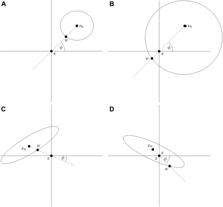
FIGURE 1. In this figure, x₀ denotes a source, x denotes the reference point, and w denotes the wavefront. (A). r (0) > 0 and r(t) = d (x, w) > 0. (B). r (0) > 0 and r(t) = d (x, w) < 0. (C). r (0) < 0 and r(t) = d (x, w) < 0. (D). r (0) < 0 and r(t) = d (x, w) > 0.

The explicit form of y (⋅, ⋅) can be obtained by integrating the equations appearing in the last display and the boundary condition that for the differential Eq. 9, Eq. 11 at t = t₀ > 0 for each angle ϕ, y (t₀, r (t₀), ϕ) = y₀(ϕ) and r (t₀) = r₀. The value of y₀(ϕ) may vary depending on the source and the epidemic under consideration, and may include values of 0 given anisotropy. First integrating Eq. 11 for a fixed ϕ gives

$\log \left(\frac{y}{1-y}\right)=-b\log \left(1+\frac{r}{g(\varphi )}\right)+c_1(\varphi )(12)$

where c₁(ϕ) is a constant of integration for fixed ϕ. Then, integrating Eq. 9 for a fixed ϕ gives

$\log \left(\frac{y}{1-y}\right)=at+c_2(\varphi )(13)$

where c₂(ϕ) is a constant of integration as in Eq. 12 for fixed ϕ. Now, combining Eq. 12, Eq. 13 and taking any convex combination of both the sides we get the generic functional form

$\log \left(\frac{y}{1-y}\right)=-b^{\prime }\log \left(1+\frac{r}{g(\varphi )}\right)+a^{\prime }t+c_3(\varphi )(14)$

that satisfies jointly the differential Eq. 9, Eq. 11. Note that, b′ and a′ are obtained such that the right-hand side of Eq. 14 is a convex combination of the right hand side terms in Eq. 12, Eq. 13 (one example is given by b′ = b/2 and a′ = a/2). Algebraic rearrangement of Eq. 14 yields that the explicit form for y (⋅) up to constants of integration for fixed ϕ is

$y(r,\varphi ,t|\mathrm{\Theta })=\frac{1}{1+{\left(1+\frac{r(t)}{g(\varphi )}\right)}^b\exp (-at)A(\varphi )}(15)$

where the parameters are a, b, g (⋅), and $A(\varphi )=\frac{1}{\exp (c_3(\varphi ))}$. The above display is a spatio-temporal process for disease intensity with spatial kernel $F(\varphi ){\left(1+\frac{r(t)}{g(\varphi )}\right)}^{-b}$ for the disease wavefront in the direction ϕ. We note that this result is a generalization of the ‘geometric’ spatial kernel considered in Rieux et al. [22] among the candidate models for anisotropic dispersal densities, wherein the function g that induces anisotropy is a radial density; Rieux et al. [22] consider the Von Mises distribution for a specific functional form.

A derived model for velocity provides a description of the movement of an epidemic wavefront relative to the reference point. As noted in the introduction, this can be especially useful for epidemiological data that are sparse in space and time. From Eq. 9, Eq. 11, the velocity of the wavefront relative to the reference point is given by

$v=\frac{dr(t)}{dt}=-M{\left(\frac{1}{g(\varphi )+r}\right)}^{-1}(16)$

where $M=\frac{a}{b}$. Integrating Eq. 16 yields

$\log \left(1+\frac{r(t)}{g(\varphi )}\right)=-Mt+h(\varphi )(17)$

where h(ϕ) is a normalizing constant for fixed angle ϕ. We note that Eq. 17 is linear in time and can be fit to obtain estimates of M, h, and g using regression methods (as described in detail below).

2.2.2 Multiple Source Model

We extend the velocity model (Eq. 17) above to describe epidemics emanating from K source points. A summary of the notations used is given in Table 1.

TABLE 1

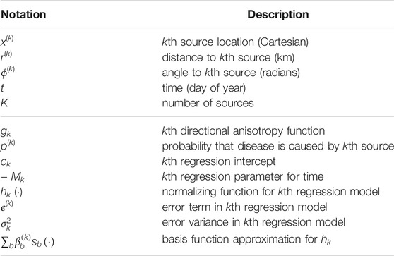
TABLE 1. Notations used in multi-source model. The horizontal line divides notations for data quantities (above) from notations for model quantities (below). In the text, subscripts i are appended to the data notations to indicate the corresponding quantity for the ith observation. Similarly, hats are placed over the model quantities to indicate estimates (e.g., ${\widehat{c}}_k$).

Let (x⁽¹⁾, …, x^(K)) denote the source locations, where $x^{(k)}\in {\mathbb{R}}^2$ for all k = 1, … , K. Now an arbitrary location (reference point) $x\in {\mathbb{R}}^2$ is associated with K pairs (r⁽¹⁾, ϕ⁽¹⁾), …, (r^(K), ϕ^(K)), where ϕ^(k) ∈ (−π/2, π/2] (resp. $r^{(k)}\in \mathbb{R}$) denotes the angular coordinate (resp. signed distance) of the kth source point x^(k) relative to x for all k = 1, … , K. A depiction of this data representation is given in Figure 2.

FIGURE 2

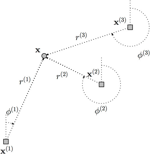
FIGURE 2. Depiction of data representation. A single location x is shown relative to three source points x⁽¹⁾, x⁽²⁾, and x⁽³⁾, and the polar coordinates (r⁽¹⁾, ϕ⁽¹⁾) (r⁽²⁾, ϕ⁽²⁾), and (r⁽³⁾, ϕ⁽³⁾) label the distances and angles to each source.

Let $\left(\right.r^{(k)}(t)$ denote the signed distance of the wavefront in the direction ${\varphi }^{(k)}\left.\right)$ at time t from the reference point x. Applying the model framework above to each set of coordinates yields the collection of velocity models

$\log \left(1+\frac{r^{(k)}(t)}{g_k({\varphi }^{(k)})}\right)=-M_{k}t+h_k({\varphi }^{(k)}),k=1,\dots ,K(18)$

Now, if multiple sources are present, any given location could be subject to disease exposure from as many as K wavefronts moving simultaneously. Yet, depending on conditions, the movement patterns of the wavefronts, and relative distances to each epicenter, an infection event at any particular time and location is attributable to the different sources with different probabilities. In other words, disease at particular locations is more likely due to certain sources rather than others. To accommodate this intuition, a latent process Z is introduced that indicates causal attribution of disease to one of the K sources with a certain probability:

$\mathbf{Z}\sim \text{Multinomial}\left(1,\left(p^{(1)},\dots ,p^{(K)}\right)\right)(19)$

For example, P (Z = 1) = p⁽¹⁾ indicates that an infection event is caused by source 1 with probability p⁽¹⁾. We then assume that a disease occurrence is described by each of the K velocity models given in Eq. 18 with probabilities p⁽¹⁾, …, p^(K). That is, for an arbitrary disease occurrence at time t, we posit the set of wavefront descriptions

$\log \left(1+\frac{r^{(k)}(t)}{g_k\left({\varphi }^{(k)}\right)}\right)=-M_{k}t+h_k\left({\varphi }^{(k)}\right)\text{with\hspace{0.17em}probability\hspace{0.17em}}{p}^{(k)}=P(Z=k)(20)$

for k = 1, … , K. This framework makes the implicit assumption that disease is caused by inoculum produced at exactly one source. However, it will be seen that our estimation method does not involve a hard classification rule for disease observations–we instead specify observation weights for each velocity model according to estimated probabilities p⁽¹⁾, …, p^(K).

2.2.3 Estimation

We propose an estimation procedure wherein velocity models are fit using regression methods conditional on g_k. The functions g_k introduce anisotropy in the model by imposing directional variation in the spatial rate of change of disease incidence via the differential equation in Eq. 11. In many applications, known variables drive anisotropy, so it is plausible to estimate g_k from covariate information or secondary data sources.

The velocity models Eq. 18 are fitted conditional on g_k to disease occurrence data (presence or absence) of the form ${\left\{(r_i^{(1)},{\varphi }_i^{(1)}),\dots ,(r_i^{(K)},{\varphi }_i^{(K)}),t_i\right\}}_{i=1}^n$ indicating the locations and times of the first observed disease case. For the purpose of exposition, suppose one is fitting only the kth model: consider just the data $(r_i^{(k)},{\varphi }_i^{(k)},t_i)$ and assume P (Z_i = k) = 1. Now, adding an offset c_k and Gaussian error term ${ϵ}_i^{(k)}$ to Eq. 18 yields the statistical data generating model

$\log \left(1+\frac{r_i^{(k)}}{g_k\left({\varphi }_i^{(k)}\right)}\right)=c_k-M_k{t}_i+h_k\left({\varphi }_i^{(k)}\right)+{ϵ}_i^{(k)}\{\begin{array}{c}{ϵ}_i^{(k)}\stackrel{iid}{\sim }N\left(0,{\sigma }_k^2\right)\hfill \\ i=1,\dots ,n\hfill \end{array}(21)$

Estimates of c_k, M_k and h_k are easily computed using semiparametric regression. Let s₁ (⋅), …, s_B (⋅) denote a set of B basis functions for the h^(k) function. Now, rewriting Eq. 21 we obtain

$\log \left(1+\frac{r_i^{(k)}}{g_k\left({\varphi }_i^{(k)}\right)}\right)=c_k+(-M_k)t_i+{\beta }_1^{(k)}{s}_1\left({\varphi }_i^{(k)}\right)+\cdots +{\beta }_B^{(k)}{s}_B\left({\varphi }_i^{(k)}\right)+{ϵ}_i^{(k)}(22)$

The ordinary least squares solution to Eq. 22 yields estimates of ${\widehat{c}}_k,{\widehat{M}}_k$ and ${\widehat{h}}_k={\sum }_b{\widehat{\beta }}_b^{(k)}{s}_b$.

Finally, this estimation strategy is extended to the full collection of K models by accounting for the latent variables Z_i that attribute each of the i data points to one of the K sources. Formally, the joint likelihood of the data arising from Eqs. 19, 20 is maximized with respect to the parameters $p^{(k)}\in {\mathbb{R}}^N$, ${\beta }^{(k)}\in {\mathbb{R}}^{B+2}$, and ${\sigma }_k^2$ for k = 1, … , K. The EM algorithm is used to iteratively update estimated multinomial probabilities ${\widehat{p}}_i^{(1)},\dots ,{\widehat{p}}_i^{(K)}$ for each data point in alternation with fitting the regression models in Eq. 22 using the estimate ${\widehat{p}}_i^{(k)}$ as a regression weight for the ith data point in fitting the kth model. In detail, the iterations are given by:

1. Initiate ${\widehat{p}}_i^{(k)}$ as the weight of ith data-point to be associated with kth source, where ${\sum }_{k=1}^K{\widehat{p}}_i^{(k)}=1$.

2. Compute/update the estimates ${\left({\widehat{c}}_k,{\widehat{M}}_k,{\widehat{h}}_k,{\widehat{\sigma }}_k^2\right)}_{k=1}^K$ by fitting each of the models in Eq. 22 using weighted least squares (WLS) with weights ${\widehat{p}}_i^{(k)}$ for the ith data point and the kth model.

3. Update ${\widehat{p}}_i^{(k)}$ by

${\widehat{p}}_i^{(k)}=\frac{\phi \left(\log \left(1+\frac{r_i^{(k)}}{g_k\left({\varphi }_i^{(k)}\right)}\right)-{\widehat{c}}_k+{\widehat{M}}_k{t}_i-{\widehat{h}}_k\left({\varphi }_i^{(k)}\right),{\widehat{\sigma }}_k^2\right){\widehat{p}}_i^{(k)}}{{\sum }_{k=1}^K\phi \left(\log \left(1+\frac{r_i^{(k)}}{g_k\left({\varphi }_i^{(k)}\right)}\right)-{\widehat{c}}_k+{\widehat{M}}_k{t}_i-{\widehat{h}}_k\left({\varphi }_i^{(k)}\right),{\widehat{\sigma }}_k^2\right){\widehat{p}}_i^{(k)}}(23)$

where φ(x, σ²) is the probability density function of a Gaussian random variable with mean zero and variance σ² evaluated at value x.

4. Repeat steps two to three until convergence.

A simple heuristic for the initialization step is to use as ${\widehat{p}}_i^{(k)}$ the estimated probabilities obtained by logistic regression of an indicator of whether the kth source is closest on the variables $r^{(1)}/{\widehat{g}}_1({\varphi }^{(1)}),\dots ,r^{(K)}/g_k({\varphi }^{(K)})$. We note that an isotropic model with one or many sources can be recovered within this framework as a special case by fixing g_k(x) = 1/2π for x ∈ [0, 2π], with the consequence that h_k ≡ 0. The details on the derivation and explanation of the fitting procedure is given in the Supporting Information S1 EM Algorithm.

2.2.4 Spatial and Temporal Predictions

Estimated models—the K models in Eq. 22 — directly yield fitted values for the quantity $\log \left(1+\frac{r_i^{(k)}}{g_k\left({\varphi }_i^{(k)}\right)}\right)$. Since this quantity does not have meaningful units, estimated times of disease occurrences conditional on location and estimated distances of occurrences from sources conditional on time and direction for each data point provide more interpretable assessments of fit quality with biological relevance. These temporal and spatial estimates are

$\begin{array}{ll}\hfill {\widehat{t}}_i^{(k)}& =\frac{1}{-{\widehat{M}}_k}\left(\log \left(1+\frac{r_i^{(k)}}{g_k\left({\varphi }_i^{(k)}\right)}\right)-{\widehat{h}}_k\left({\varphi }_i^{(k)}\right)-{\widehat{c}}^{(k)}\right)\hfill \end{array}(24)$

$\begin{array}{ll}\hfill {\widehat{r}}_i^{(k)}& =g_k\left({\varphi }_i^{(k)}\right)\left(\exp \left\{{\widehat{c}}^{(k)}-{\widehat{M}}_k{t}_i+{\widehat{h}}_k\left({\varphi }_i^{(k)}\right)\right\}-1\right)\hfill \end{array}(25)$

Since the model includes estimated probabilities that the ith data point is associated with each source (the estimates ${\widehat{p}}_i^{(1)},\dots ,{\widehat{p}}_i^{(K)}$), a simple heuristic for selecting a single temporal estimate from ${\widehat{t}}_i^{(1)},\dots ,{\widehat{t}}_i^{(K)}$ and a single spatial estimate from ${\widehat{r}}_i^{(1)},\dots ,{\widehat{r}}_i^{(K)}$ is to choose the estimates ${\widehat{t}}_i^{(k)}$ and ${\widehat{r}}_i^{(k)}$ associated with the most probable source. That is, let

$({\widehat{t}}_i,{\widehat{r}}_i)\stackrel{\text{def}}{=}\left({\widehat{t}}_i^{(k^{*})},{\widehat{r}}_i^{(k^{*})}\right)\text{\hspace{0.17em}where}{k}^{*}=\underset{k}{\mathrm{arg\; max}}\left\{{\widehat{p}}_i^{(k)}\right\}(26)$

Then, a fitted model can be evaluated according to the temporal and spatial root mean square error (RMSE) metrics.

$\begin{array}{l}\hfill {\text{rmse}}_t\stackrel{\text{def}}{=}{\left(\frac{1}{n}\sum _{i=1}^n{(t_i-{\widehat{t}}_i)}^2\right)}^{1/2}\end{array}(27)$

$\begin{array}{l}\hfill {\text{rmse}}_r\stackrel{\text{def}}{=}{\left(\frac{1}{n}\sum _{i=1}^n{(r_i-{\widehat{r}}_i)}^2\right)}^{1/2}\end{array}(28)$

As we describe below, we used RMSE for model comparison because our interest is in prediction accuracy and RMSE is a direct measurement of this quantity.

2.3 Cucurbit Downy Mildew Data

Epidemics of cucurbit downy mildew recorded in the U.S. from 2008 to 2016 were obtained from the data submitted to the Cucurbit Downy Mildew ipmPIPE program (http://cdm.ipmpipe.org). The ipmPIPE is an information and decision support system that gathers pertinent data (disease occurrence in cucurbit production areas), applies predictive models to the data, incorporates expert interpretation, and communicates near-real-time output to cucurbit growers, extension personnel, and crop consultants [11]. Records in the system include disease reports from a network of regularly monitored sentinel plots as well as voluntary disease reports from non-sentinel plots submitted by commercial growers, agricultural researchers, and the general public. We describe below the two types of disease reports and a subset of the data selected for analysis.

2.3.1 Sentinel Plot Reports

Sentinel plots were fixed locations planted with different cucurbit host types for monitoring downy mildew outbreaks and were strategically placed within specific states at locations that collaborators could easily access. During the years 2008–2016, the sentinel plots were located at research facilities or in commercial fields with standard dimensions of 15 m × 61 m and were georeferenced using the Global Positioning System. These plots were monitored for disease symptoms weekly to biweekly by cooperating scientists and extension specialists and were planted with susceptible, early maturing cultivars. The cucurbit host types grown in the sentinel plots were Cucumis sativus (cucumber cv. Straight 8 and Poinsett 76), Cucumis melo (cantaloupe cv. Hales Best Jumbo), Cucurbita pepo (acorn squash cv. Table Ace), Cucurbita maxima (giant pumpkin cv. Big Max), Cucurbita moschata (butternut squash cv. Waltham), and Citrullus lanatus (watermelon cv. Micky Lee) [11]. The compiled data set on sentinel plot disease reports consist of the date of first observed occurrence of disease, the reporting date, affected host type, the incidence of plants affected, and plot location.

2.3.2 Non-Sentinel Reports

Cucurbit downy mildew was also monitored via voluntary reporting in locations not designated for regular surveillance. These locations include commercial fields, research plots, and home gardens. Compiled data on voluntary reports consisted of the date of first observed occurrence of disease, the reporting date, location, and affected host type (if provided). This information is potentially instructive for understanding the distribution and appearance of cucurbit downy mildew, but subject to greater uncertainty with respect to the timeliness of disease detection due to the non-standardized nature of the plant populations, potential confounding from fungicide applications, and the absence of regular monitoring and reporting protocols.

2.3.3 Data Selected for Analysis

We selected a subset of the disease reports from which to model epidemic wavefronts using the framework described above. The subsetting strategy was intended to capture a single epidemic wave as best as possible while ensuring uniform reliability on the timeliness of reports. First, for the reliability of timeliness, we considered only sentinel reports. This was thought to better ensure consistent variation across reports in the accuracy of dates of first observed disease occurrences due to a fixed observation frequency and protocol. Second, late-season outbreaks are known to occur due to later-planted cucurbit crops that are common in southern and mid-Atlantic regions of the U.S [1]). Thus, we sought to capture the first outbreak each year by restricting attention to reports in which the date of observed occurrence is before August. Finally, we selected data from 2008, 2009, and 2010 to capture annual variation, and chose these specific years due to a relatively greater number of sentinel plots available (n = 25, 65, and 28, respectively). From the resulting reports, we compiled data on the location, date of symptom onset (presence of disease at any level), and host type from each report (Figure 3).

FIGURE 3

FIGURE 3. Disease reports from 2008 to 2010 plotted by location, reported symptom date, and plot type.

2.3.4 Application Details

The three consecutive years of selected sentinel reports were analyzed separately by fitting isotropic (I) and anisotropic (A) one-source (OS) and two-source (TS) velocity models to data from each year. To apply the model framework to this specific dataset, we identified potential source locations from an exploratory analysis of early occurrences and developed a simple method of estimating the functions g_k from meteorological information known to drive dispersal.

2.3.5 Selection of Source Locations for Cucurbit Downy Mildew Data

Source locations were specified as county centroids. To identify putative source locations for each year, we examined both sentinel and voluntary reports of early disease occurrences for geographical location and timing. The first observation of disease occurrence occurs reliably in southern Florida every year, so the centroid of the county in which the first disease symptoms were reported each year was fixed as the (anonymized) main source point. In addition, early occurrences are often observed in the southwestern U.S. and the Great Lakes region before expected dispersal from the source point in Florida. We identified several counties in northern latitudes (Erie and Wayne Counties in Ohio, and Niagara County in New York) that had early occurrences in multiple years, and several counties in the southwestern region (Brazos and Hidalgo Counties in Texas, Vernon County in Louisiana, and Payne County in Oklahoma) that had early occurrences in multiple years. We considered each of these counties as possible locations for a second source in each year informed by biology of the pathosystem [13, 14, 26]. Based on the reports in each region, the earliest disease occurrences were used to identify dates at which a putative source in each region might appear. We note here that the alternate sources specified are not necessarily the actual location of overwintering of P. cubensis, but are a reasonable proxy for an alternate source of inoculum, if one should exist, when placed within the path of the wavefront emanating from the true source.

2.3.6 Estimation of Anisotropy Function From Meteorological Data

While estimating the parameters ${\left({\left\{p_i^{(k)}\right\}}_{i=1}^n,{\widehat{c}}_k,{\widehat{M}}_k,{\widehat{h}}_k,{\widehat{\sigma }}_k^2\right)}_{k=1}^K$ in the EM algorithm, the functions ${(g_k)}_{k=1}^K$ were considered known. However, usually g_k are not known, so we propose estimating g_k using some additional data. In our application we estimated the functions g_k based on meteorological data measured at the source locations, since variation in wind direction and speed are primary drivers of anisotropic dispersal in this pathosystem. Hourly wind direction and speed near each county centroid with a sentinel plot or imputed disease source was derived from weather observations in the National Oceanic and Atmospheric Administration Integrated Surface database [28] and were provided by BASF (Research Triangle Park, Raleigh, NC).

We modeled g_k as radial density functions and estimated g_k using the wind data. Nonparametric kernel density estimates of the radial density functions g_k were computed from the collection of hourly wind directions at each of the k sources over the time interval represented in the disease data. If ${\theta }_i^{(k)}$ denotes the angle of the predominant wind direction at time point i and source location k, the wind direction data ${\theta }_1^{(k)},\dots ,{\theta }_n^{(k)}$ is treated as a sample of size n_k on the unit circle centered at the source point x^(k). For each k, we computed a kernel density estimator ${\widehat{g}}_k$ of the form

${\widehat{g}}_k(x)=\frac{C(h)}{n}\sum _{i=1}^{n_k}K\left(\frac{1-x{\theta }_i^{(k)}}{h^2}\right),x\in [\mathrm{0,2}\pi ](29)$

where h is a positive number and $C{(h)}^{-1}={\int }_0^{2\pi }K\left((1-x\theta )/h^2\right)d\theta$ is a normalizing constant. For the application in this work, the kernel function K(z) = exp{ − z} is used.

2.3.7 Application of Model Framework

To apply our modeling framework in the analysis of the cucurbit downy mildew data, we calculated two alternate responses: a response for the isotropic models, $\log \left(1+r_i^{(k)}\right)$, and a response for the anisotropic models, $\log \left(1+r_i^{(k)}/{\widehat{g}}_k\left({\varphi }_i^{(k)}\right)\right)$ for each data point i = 1, … , n, and estimated the velocity models as described above.

2.4 Simulation Study

We conducted a set of simulations to quantify parameter recovery using the model and estimation procedure for different sample sizes and scenarios when disease spread was weakly to strongly anisotropic. First, we set two source locations well separated in two-dimensional space at Cartesian coordinates of (0,0) and (2000, 2000) representing the first and second sources, respectively. These locations approximate the spatial scale in kilometers of the cucurbit downy mildew sources in Florida and an alternate source of interest in the Upper Midwest. For sample sizes of n = 50, 100, 250, and 500, we fixed the proportion of disease attributable to the first and second sources as 0.7 and 0.3, respectively. We chose the Von Mises density function to generate circular normal data that could induce anisotropy in disease spread relative to the two locations. The Von Mises function has two parameters: μ, a location measure, and κ, a concentration measure, and is given by

$f(x)=\frac{e^{\kappa \cos (x-\mu )}}{2\pi I_o(\kappa )}$

for any angle x ∈ [μ − π, μ + π] where I_o is a Bessel function of order 0. The μ values were chosen such that disease spread from the two sources would be in opposite directions and overlapping in space by setting ${\mu }_1=\frac{\pi }{4}$ and ${\mu }_2=\frac{5\pi }{4}$. Values of κ = 5 and κ = 2 were chosen to produce strongly and weakly anisotropic spread, respectively. We generated two separate angle grids from the uniform distribution and used the Von Mises density function with μ and κ as noted to estimate g(ϕ).

We also simulated temporally synchronous and asynchronous epidemics by varying the daily time grids from the uniform distribution. The time grid ranged from the day of year 50–150 for synchronous spread from the two sources, and days 50–150 for source 1, and days 100–150 for source 2 for asynchronous epidemics. We then generated data according to the two models by inputting the corresponding time grid, angle grid, and coefficients according to a simplified version of the model in Eq. 21.

We consider that the error variance σ² is the same for both the sources. We evaluated the sensitivity of the parameter estimates to error variance by varying σ² two-fold. The distance from each source location (r) was then calculated by back transforming r. We then calculated the corresponding x and y Cartesian coordinates.

We pooled the simulated Cartesian coordinates and times, converted the Cartesian coordinates to sets of polar coordinates for each source, and applied the fitting procedure to estimate coefficients. We ran 1,000 simulations and calculated the mean and standard deviation of the estimated coefficients, as well as the proportion of the n samples attributed correctly to each of the two sources in each of the 1,000 simulated epidemics. Examples of individual simulations are presented in Figure 4.

FIGURE 4

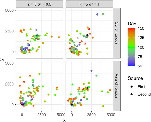
FIGURE 4. The locations of observations from one simulation for κ = 5 and σ² = 0.5 and 1. The results are shown for temporally synchronous and asynchronous epidemics. The x and y axis scales are set to -500 and 5,000 for better visualization. Note that x and y are coordinates in this visualization.

3 Results

In this section, we first present representative conditions important for confirming the performance of the two-source model and the EM procedure for parameter recovery and source attribution. Full results of other simulation experiments are presented as Supporting Information. Following the simulation results, we present the results of analyses of observed disease data from 2008 through 2010. For each year, several candidate models were fit. We considered both one-source and two-source models in each year, and anisotropic and isotropic versions of each. In addition, for the two-source models, we considered two alternate source locations based on the considerations discussed above.

3.1 Simulation Study

The mean and standard deviation of the estimated coefficients for n = 50 and 250 for a two-source epidemic with anisotropic spread of disease (Von Mises distribution κ = 5) are given in Table 2. Results for n = 100 and 500 are given in Supplementary Table S1 and results for κ = 2 are given in Supplementary Figures S1–3. Parameter estimates were generally accurate across the various sample sizes and whether epidemics at the two sources were initiated synchronously or asynchronously, but sensitive to error variance. There was a slight increase in the mean values of the intercept estimates as n increased from 50 to 250, particularly as the error variance increased. Expectedly, the standard deviation of the parameter estimates increased with error variance and decreased with n. Overall, the estimates were highly accurate in all scenarios except for large sample sizes with high variance and an asynchronous start (n = 250, σ² = 1). We hypothesize that the disease observations become more densely mixed under this setting and thus make the sources more difficult to discern, thereby compromising estimation of model parameters. We note in particular that estimates for the less dominant source (source 2) are most severely compromised, consistent with our observation below that more challenging simulation conditions tend to cause misattribution to the dominant source.

TABLE 2

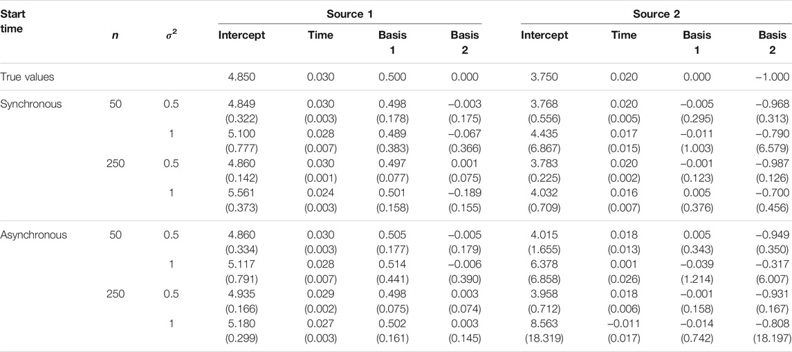
TABLE 2. The mean parameter estimates and standard deviation for two-source models fit to simulated data. Two sets of estimates are reported corresponding to a (0,0) placement for a first source and a (2000,2000) placement for a second source, with temporally synchronous or asynchronous epidemics (n is the sample size.)

The estimated probability of disease being due to spread from one of the two sources was used to attribute disease to each of the sources in the simulations and calculate the overall mean proportion of disease correctly assigned to the true source (Figure 5 and Figure 6). The disease due to the dominant source, source 1, was attributed correctly to this source in most simulations independent of sample size, error variance, location of the source, or other epidemic conditions specified. This behavior is consistent with expectations, as without additional information the EM algorithm attributes disease due to the most abundant, dominant inoculum source. The disease was less often attributed correctly to the less abundant second source, although source attribution here was still relatively accurate. Classification accuracy was sensitive to the placement of sources in space, diminishing as the two sources were more closely situated. Classification accuracy decreased when epidemics initiated from the two sources were temporally asynchronous, anisotropy was stronger, and error variance was larger. Although we see that some of the observations from the less abundant source can be incorrectly allocated to the more abundant source, the estimates of the model parameters for the two sources are still relatively accurate and capture the behavior of the spread from each of the sources in terms of velocity of spread and anisotropy.

FIGURE 5

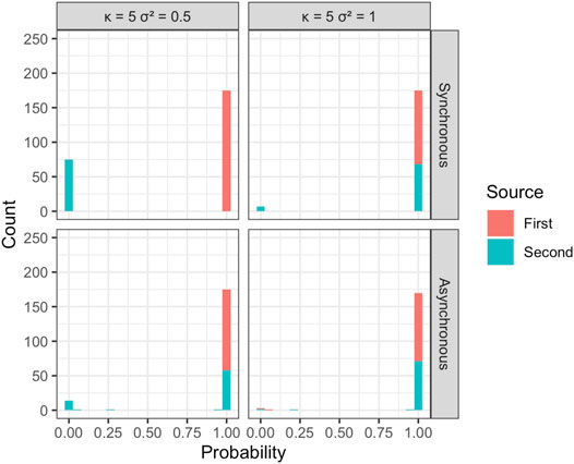
FIGURE 5. Estimated probability of disease source for each of the n = 250 observations in individual, representative simulations with κ = 5 and σ² = 0.5 and 1. Results are shown for temporally synchronous and asynchronous epidemics.

FIGURE 6

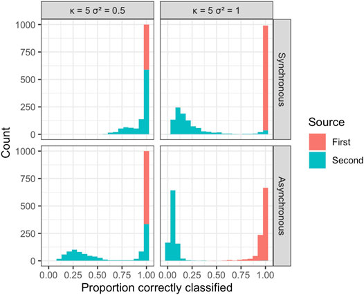
FIGURE 6. Results from a simulation experiment with n = 250; κ = 5, two levels of error variance (σ²), and temporally synchronous or asynchronous epidemics. The histogram summarizes the mean proportion of disease correctly assigned to the true source over 1,000 simulations.

3.2 Estimation for Cucurbit Downy Mildew Dataset

Parameter estimates are reported for six models in each year: three isotropic models having one source only, an alternate source in the north, and an alternate source in the southwest; and three anisotropic models with the same source locations. The isotropic models are referred to as “Isotropic One Source” (IOS), “Isotropic Two Source (Southwest)” (ITS-SW), and “Isotropic Two Source (North)” (ITS-N); and similarly, the anisotropic models are referred to as “Anisotropic One Source” (AOS), “Anisotropic Two Source (Southwest)” (ATS-SW), and “Anisotropic Two Source (North)” (ATS-N). For the two-source models, separate velocity models are fitted corresponding to each of the two sources, and these are distinguished by indicating the source location parenthetically, e.g., ITS-SW (FL) and ITS-SW (TX) indicate the two velocity models that comprise the ITS-SW model. Since one of these sources is always located in Florida in the analyses, we adopt the convention of referring to the two sources as the Florida source and the “alternate” source.

Graphical and tabular representations of spatial and temporal prediction errors are reported for each of the models fitted to data from each year. The graphical representations focus on temporal predictions and show contours of the estimated epidemic fronts at various times. Numerical reports include spatial prediction errors, and, for the two-source models, errors from models fitted using additional alternate source locations that were considered.

These results simultaneously address several questions. First, the model comparisons suggest whether in a given year dispersal exhibited directional variation. Second, the same comparisons provide indirect evidence for the existence of a second source, depending on whether positing such a source better explains the pattern of dispersal. Third, the prediction errors illustrate the sensitivity of results to the placement of source locations.

3.3 Disease Outbreak and Spread for Cucurbit Downy Mildew Dataset

In all the years, the disease was observed first in Florida from January to February, with reports in sentinel plots beginning in February to March (Figure 3). The first detection of the disease generally progressed northward with time, but with some exceptions particularly in the southwestern locations along the Gulf Coast and infrequently in the Great Lakes region such as in 2009. That is, there appeared to be anisotropy in disease spread.

3.3.1 Model Fitting for Cucurbit Downy Mildew Dataset

The parameter estimates for one- and two-source isotropic and anisotropic models fitted to data from each of the years 2008 through 2010 are given in Table 3, Table 4, and Table 5. For all years, the time parameter estimates ($-{\widehat{M}}_k$) for the isotropic and anisotropic one-source models (IOS and AOS) were significant, indicating that the Florida source is an important epicenter in explaining disease progression. Further, the estimates of this parameter were not affected considerably by model specification—that is, they are relatively stable across models in each year—suggesting that the epidemic velocity associated with the Florida source is a relatively strong signal in the data.

TABLE 3

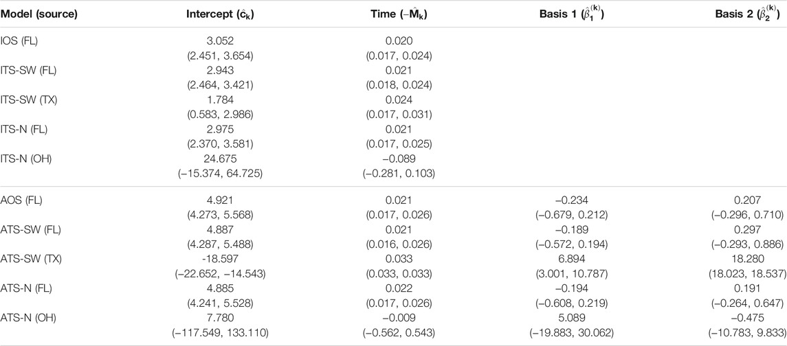
TABLE 3. Parameter estimates and 95% confidence intervals for one- and two-source models fit to 2008 data (n = 25). In the two-source models, two sets of estimates are reported corresponding to a northern placement and a southwestern placement for the alternate (non-FL) source. No basis parameters are reported for the isotropic models, since these terms are only included in the anisotropic models (FL - Florida, TX - Texas, OH - Ohio).

TABLE 4

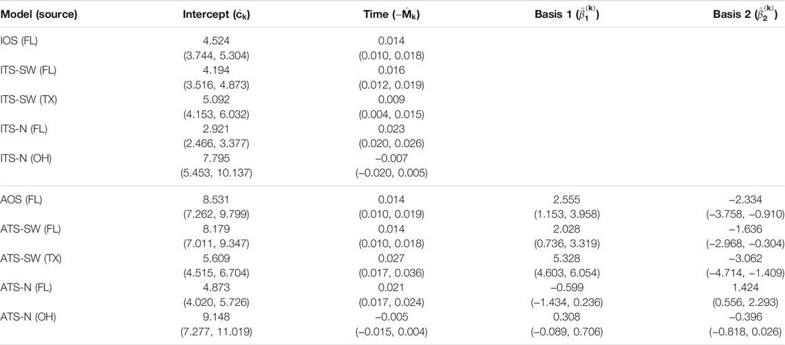
TABLE 4. Parameter estimates and 95% confidence intervals for one- and two-source models fit to 2009 data (n = 65). In the two-source models, two sets of estimates are reported corresponding to a northern placement and a southwestern placement for the alternate (non-FL) source. No basis parameters are reported for the isotropic models, since these terms are only included in the anisotropic models (FL - Florida, TX - Texas, OH - Ohio).

TABLE 5

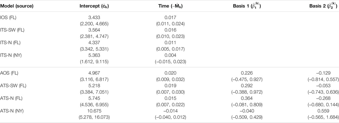
TABLE 5. Parameter estimates and 95% confidence intervals for one- and two-source models fit to 2010 data (n = 28). In the two-source models, two sets of estimates are reported corresponding to a northern placement and a southwestern placement for the alternate (non-FL) source. No basis parameters are reported for the isotropic models, since these terms are only included in the anisotropic models. In this year, no alternate source model is estimated for the southwest location, as nearly all data points are attributed to the FL source during model fitting (FL - Florida, TX - Texas, OH - Ohio).

For the two-source models, estimates of the time parameter associated with the alternate source were not significantly different from 0 when the alternate source was placed in the Great Lakes region (ITS-N and ATS-N in all years). This indicates that the data provide little evidence of dispersal emanating from the northern alternate source location, suggesting that no epicenter was present, or detectable, in the region. In these cases, when the northern source is included in the model, the contribution of the associated velocity model in explaining disease progression is to generate predictions of occurrences at time-invariant distances from the source based on certain observations in the dataset. In many cases, the estimated parameter was negative, indicating a slightly contracting front toward the source. By contrast, time parameters associated with the alternate source were positive and significant when the alternate source was placed in the southwest (ITS-SW and ATS-SW in 2008 and 2009; the estimated ITS-SW or ATS-SW models in 2010 reduced to single-source models, as all data points had low estimated probabilities of being caused by a southwestern source).

The basis parameter estimates ${\widehat{\beta }}_1^{(k)}$ and ${\widehat{\beta }}_2^{(k)}$, which when combined give estimates of the normalizing functions ${\widehat{h}}_k$, are of varying significance depending on the year and velocity model. In 2008, these parameters are only significant for the ATS-SW model; in 2009, they are significant for every model except ATS-N; and in 2010, they are not significant for any model. Since the normalizing functions h_k are functions of angle, the significance of these parameters indirectly indicates the statistical strength of evidence that anisotropy is present. Thus, in 2008 there is evidence for anisotropic spread from the southwestern source, and in 2009, there is evidence of anisotropic spread from all source locations.

Finally, the estimates for the two-source models suggest that the importance of including a second source varies depending on the year and source location. None of the velocity models associated with northern source locations had significant non-intercept parameter estimates. In 2008 and 2009, the velocity model associated with the Texas source included significant terms. Yet, in 2010, the ITS-SW and ATS-SW models attributed all data points to the Florida source.

3.3.2 Spatial and Temporal Predictions for Cucurbit Downy Mildew Dataset

Estimated epidemic fronts from each of the six models discussed above for each of the years 2008–2010 are shown in Figure 7, Figure 8, Figure 9, respectively, along with time-of-occurrence errors for each data point. Epidemic front predictions and associated errors for an extension of the methods to a three-source model are given in Supplementary Figure S4. Anisotropy in disease spread was apparent in the models accounting for an unequal velocity of spread in space, with the direction and magnitude varying depending on the specific source or combinations of sources (regardless of the significance of the estimates of h_k). Predicted expansion of the epidemic wavefront indicated an acceleration of epidemic velocity over time from the initial disease focus when the focus was placed in the southwest extent of the spatial domain or Florida. This was true for all years and models, consistent with the positive sign of the coefficient for the time variable associated with these models and sources ($-{\widehat{M}}_k$ in Tables 3–5). In contrast, disease sources placed in a northern location near the Great Lakes only displayed this behavior (an expanding predicted wavefront) in 2010. In 2008 and 2009, the predicted wavefronts were either little changed over time (2008) or indicated a gravitational pull behavior (2009) due to near zero or negative parameter estimates for the time parameter (Tables 3, 4).

FIGURE 7

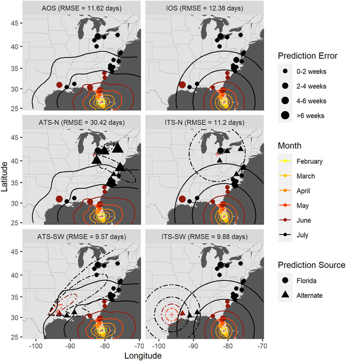
FIGURE 7. Time-of-occurrence prediction errors for predictions from isotropic and anisotropic one- and two-source models fit to data from sentinel plots in 2008, with contours representing estimated disease front over time according to the models. The two-source models were each fit with two alternate (non-FL) source locations: a northern and a southwestern location. Each panel shows results according to a different model: isotropic one-source (IOS); isotropic two-source (ITS); anisotropic one-source (AOS); and anisotropic two-source (ATS).

FIGURE 8

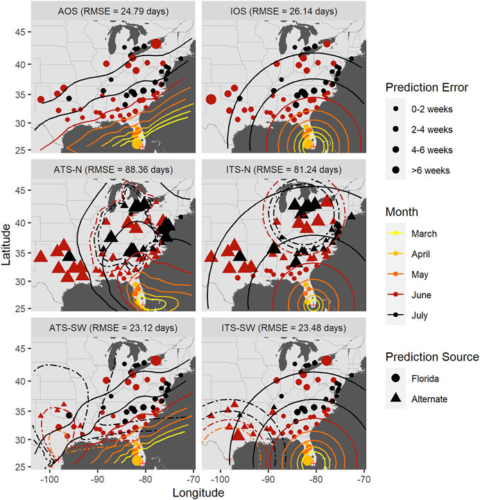
FIGURE 8. Time-of-occurrence prediction errors for predictions from isotropic and anisotropic one- and two-source models fit to data from sentinel plots in 2009, with contours representing estimated disease front over time according to the models. The two-source models were each fit with two alternate (non-FL) source locations: a northern and a southwestern location. Each panel shows results according to a different model: isotropic one-source (IOS); isotropic two-source (ITS); anisotropic one-source (AOS); and anisotropic two-source (ATS).

FIGURE 9

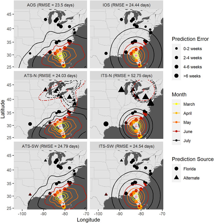
FIGURE 9. Time-of-occurrence prediction errors for predictions from isotropic and anisotropic one- and two-source models fit to data from sentinel plots in 2010, with contours representing estimated disease front over time according to the models. The two-source models were each fit with two alternate (non-FL) source locations: a northern and a southwestern location. Each panel shows results according to a different model: isotropic one-source (IOS); isotropic two-source (ITS); anisotropic one-source (AOS); and anisotropic two-source (ATS).

Accounting for anisotropy in one source models reduced RMSE measured in time slightly (0.76–1.35 days) but consistently (Table 6; Supplementary Figures S5–7); spatial errors were not consistently reduced in these data sets. For multiple source models, prediction errors in time and space varied over orders of magnitude depending on the model and specific year (Figures 7–9 and Table 7). Among the multiple source models, some anisotropic models reduced temporal and spatial errors for some years as compared to the corresponding isotropic model. However, no single more complex model consistently reduced prediction errors across all years when multiple sources were included.

TABLE 6

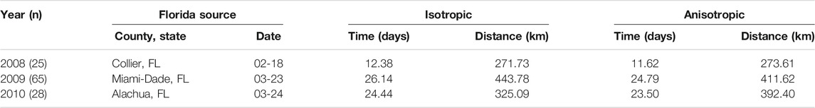
TABLE 6. Root mean square errors of time and distance for isotropic and anisotropic one-source models. The source location and time of appearance, shown in the table, are the earliest occurrences among all sentinel plots in the data for the corresponding year (n is the sample size.)

TABLE 7

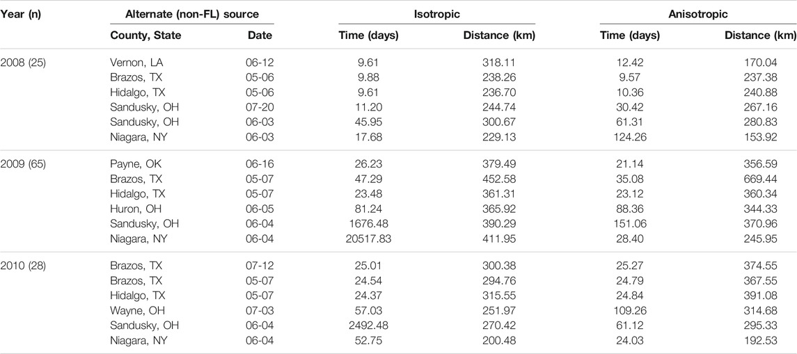
TABLE 7. Root mean square errors of time and distance for isotropic and anisotropic two-source models for several alternate source locations. The other of the two sources is placed in Florida in the same location and time as in the one-source model.

RMSE for multiple source models was sensitive to the placement of the alternate source in both space and time (Table 7). Model sensitivity to source placement was particularly acute for alternate sources placed in northern latitudes. Imputing sources in certain locations and times led to massive prediction errors in some instances, for example, when the source was placed in Niagara County, New York in 2009. Generally, reductions in RMSE in space or time were most often observed with two-source models when disease spread was isotropic and the second source was placed in the southwestern extent of the spatial domain. Conversely, the two-source models with the largest RMSE were most often associated with an alternate source sited in a northern latitude (Table 7; Figures 7–9).

3.3.3 Source Attribution

The modeling framework includes the estimation of the most probable source k resulting in disease at a distant location when multiple sources are specified. Disease outbreak was attributable to different primary sources depending on the year, location of the alternate source, and anisotropy (indicated by plotting character in Figures 7–9). Disease outbreaks in Florida and other southeastern states were invariably attributed to the source in southern Florida, independent of anisotropy or the specification of another source. In other regions, the source deemed most probable for disease outbreak at a given location depended on where sources were placed. Proximity was associated with whether a source was the most probable cause of disease at a given sentinel plot, but with some notable exceptions. For instance, setting a source in the Great Lakes region led to most disease outbreaks in the Upper Midwest, Northeast, and northern mid-Atlantic region to be attributable to the northern source rather than a source in Florida. With an alternate source sited in the southwest, plots on the western and northern edge of the Gulf Coast were mostly attributed to this source, with ensuing disease spread to the northeast (Figure 7) or north (Figure 8). In 2010 there were no contours associated with the southwest source (Figure 9) as only two sentinel plots in Texas and Michigan were attributed to that source.

We again emphasize here that prediction errors associated with any of these models varied depending on the year and specific model, and were not necessarily improved uniformly as compared to the corresponding isotropic one source model (Tables 6, 7).

4 Discussion

We have developed a generalized, wide, and flexible class of spatio-temporal models capable of accounting for the presence of any number of initial inoculum sources and any kind of anisotropic spread of biological species that can govern disease (or other) gradients and spatial spread in time. We have also built a data-driven procedure, which selects an appropriate model from the above-mentioned class of models and provides computationally efficient estimates of the model parameters. This framework is well suited to infer the probable sources of disease spread due to long-distance dispersal responsible for later outbreaks at distant locations. We successfully applied this approach to predict the spread of cucurbit downy mildew in the eastern U.S., although the class of models and estimation methods are directly applicable to any disease organism where long-distance dispersal may occur. The novelty of the class of models and estimation framework is multi-fold, as we describe below.

Previous models that describe or predict the extent of disease spread and velocity of epidemics assume dispersal is isotropic [1, 7, 8]. This assumption usually is unrealistic because wind tends to be directional, weather gradients exist, host connectivity is patchy, inoculum source strength varies between field and regions, and landscape and terrain features influence transport and deposition of inoculum [29, 30]. Anisotropy may occur at multiple spatial scales, ranging from individual plants [31], individual fields [23, 32], the mesoscale [33], and the landscape or continental scale [8, 34]. Soubeyrand et al. [21] and Rieux et al. [22] incorporated anisotropy into their models for describing disease gradients resulting from dispersal due to essentially one generation of a plant pathogenic fungus but did not consider anisotropy in epidemics over time. The models derived in this study accommodate both spatial and temporal components. The anisotropic model framework assumes that the rate of change of disease incidence with distance from a source depends on the direction. The rate of change with time is independent of location in the present framework but could be modified to allow the rate of change of disease incidence with distance to depend both on direction and time provided a richer data set for parameter estimation.

The importance of accounting for anisotropy will vary depending on the specific system under investigation. In the motivating example of cucurbit downy mildew used here, there was a small but consistent reduction in temporal prediction errors by incorporating anisotropy in disease spread. A reduction of multiple days is biologically relevant for aerially dispersed organisms with high reproductive potential and short generation times, where even a brief lag in implementing control measures may substantially diminish the efficacy of control measures and containment [5, 17, 35]. In settings where improvements in prediction errors are inconsequential or variates related to anisotropy are unknown, an isotropic, one-source model can be recovered easily in our modeling framework as a special case.

A second novel aspect of the modeling framework derived in this study is the ability to account for multiple inoculum sources that may each produce epidemic wavefronts. Interpretation of disease gradients under natural conditions has long been recognized as a difficult process due to the potential for asynchronous and overlapping wavefronts from multiple inoculum sources [16, 24]. The latent process introduced in our modeling framework assumes multiple sources may exist, which might better reflect conditions in natural environments when an organism is naturalized and primary inoculum is dispersed (e.g., [33, 36–38]). Our modeling framework is amenable to inference about the likelihood of disease outbreak at a specific location due to disease at multiple potential sources. This is often a basic question in invasion biology of immense importance for formulating effective management policies [38, 39], but a difficult question to address due to the stochastic nature of long-distance dispersal and technical challenges associated with its detection [40]. With multiple sources specified, our modeling approach attributes a probability to the first occurrence of the disease being associated with the specified sources. The simulation experiments indicate that the accuracy of source prediction can be influenced by the spatial proximity of the disease sources, temporal asynchrony of epidemics, the strength of anisotropy, and error variance. Source attribution is most accurate when sources are well separated in space, epidemics are temporally synchronous, and disease spread is isotropic. Source attribution error rates will increase when epidemic conditions vary in one or more of these characteristics, usually resulting in incorrect attribution of disease to the most dominant source in the landscape.

We considered examples with two sources in this work, but the approach is readily extendable to many sources provided a sufficiently dense data set for estimating the full set of models and associated latent variable process. As an example, we fit a three-source anisotropic model with epicenters placed in southern Florida, southern Texas, and a northern source in Ohio (Supplementary Figure S4). The model was fit successfully, and disease in nine sentinel plots was attributed to the northern source. However, all but one of these plots were located far south of the source location. Further, the coefficient of the estimated time parameter in this model for the northern source was negative, resulting in a contracting epidemic front. In this specific example, the statistical fit of the model was improved with three sources but the model predictions were not consistent with disease biology and ecology. However, the methodological aspects remain valid and should be suitable for other applications where sufficient data exists to avoid model overfitting.

A salient point here is that the modeling framework estimates the likelihood that the first occurrence of disease originated from a specific source, but does not partition total disease intensity to one or more sources or consider later pathogen incursions. The total amount of disease at a given location can be due to multiple sources with inoculum arriving at different times. Furthermore, most disease at a location may be due to secondary or community spread following an initial infection event depending on the time since that infection and local conditions (e.g., [37, 38, 41]). Nonetheless, understanding which source is most likely responsible for the first appearance of disease remains highly important for understanding potential genetic founder effects, genotypic and phenotypic traits of a newly arrived pathogen causing disease, and planning mitigation strategies.

In the motivating example of cucurbit downy mildew, there is speculation and circumstantial evidence that inoculum sources outside of Florida may be important for disease in more northern latitudes in the U.S [13, 14]. Greenhouse cucumber production has been postulated as a possible alternate source of inoculum responsible for outbreaks of cucurbit downy mildew in the Great Lakes region [13, 17, 42]. Downy mildew can occur at damaging levels in greenhouse-grown cucurbits [14], and thus winter and spring cucurbit production in protected cultivation in the Great Lakes region [43] could be a possible source of inoculum [1, 14]. Definitive evidence for this hypothesis has been elusive, though [17]. The present data set and analysis do not provide evidence of an annually-occurring, alternate source of P. cubensis in northern latitudes. In certain years downy mildew was observed in the Upper Midwest in June before the expected occurrence of a disease wavefront originating from southern Florida. However, two-source models with an observed or imputed alternate source placed in the Great Lakes region generally had the largest prediction errors, and in some cases, these errors were indeed massive. We explored various spatial placements of alternate sources in northern latitudes (north, south, east, and west of Lake Erie) and timings for their appearance based on when sporangia of P. cubensis may be in the air [44, 45]. None of the observed or imputed sources led to appreciable improvements in prediction. The three-source model we fitted also failed to yield biologically plausible predictions of disease spread associated with a northern source (Supplementary Figure S4). However, given the sparsity of the present data sets, absence of disease reports from greenhouses in the Cucurbit Downy Mildew ipmPIPE system, and our restriction of disease to the first planting of cucurbits, we caution that a lack of evidence for a second source in northern latitudes does not prove that one does not exist.

We did find support for an alternate inoculum source on the western edge of the Gulf of Mexico. This is perhaps unsurprising given that hosts of P. cubensis are present year-round in frost-free areas along the southern Gulf Coast [17]. Depending on seasonal wind direction, the southwestern source is predicted to be a source for downy mildew in the southern plains, lower Midwestern states, and certain other regions of the southeastern U.S. Separate spatio-temporal analyses also suggest that inoculum sources in the southern U.S. outside of Florida may be responsible for disease outbreaks in more northern latitudes [12]. In all years, predicted wavefronts from the southwestern source and Florida overlapped as early as May to June, potentially resulting in population admixture. Genetic evidence suggests that populations of P. cubensis in Florida may be differentiated from populations in Texas and certain other states [46]. A partial explanation for this genetic differentiation may be the presence of distinct overwintering populations and epidemic trajectories of downy mildew on the western and eastern edges of the Gulf of Mexico.

The multiple source modeling framework we present is most useful for post hoc analysis of epidemics rather than prediction. This is because parameter estimation requires an iterative procedure based on the known distribution of disease, which precludes prediction during an active epidemic. This has no bearing on one-source models, with or without anisotropy, which our analyses suggest may be adequate in some situations.

We introduced anisotropy in disease spread through the functions g_k that are estimated from prevailing wind directions at the epicenters. Wind direction and velocity at a primary inoculum source are associated with the shape of disease gradients when measured at the scale of individual or multiple fields [22, 47]. Wind speed and direction are also predictive of disease transmission of aerially dispersed pathogens at the mesoscale [33] and landscape-level [34]. At these scales and the scales we evaluated, wind direction alone is only a simple correlate of a complex biophysical process that may act along the entire path of dispersal [13, 17, 48, 49]. More fundamentally, anisotropy in the early stages of an epidemic appears to be important for dispersal patterns that persist throughout the entire epidemic. It is unclear whether this observation is idiosyncratic to these particular data sets or suggestive of a more basic process of epidemic spread being heavily affected by properties of the initial disease epicenter.

We also point out that many other functions could be used to introduce anisotropy; van Putten et al. [20] provide several useful statistical alternatives that do not explicitly consider wind. As discussed above, physical process models could better capture anisotropy due to environmental factors but at the expense of greater data and computational requirements [48]. Similarly, knowledge of host presence and their disease status in the landscape and more intensive placement and sampling of sentinel plots could enable one to develop time-varying anisotropy functions not possible here due to the extent of the cucurbit downy mildew data sets. In spite of these limitations, the novelty and utility of our modeling framework is that it is tractable for estimating the generalized location and velocity of a disease front from sparsely sampled data with minimal data acquisition costs. Furthermore, when multiple sources exist the most probable source of the initial appearance of disease can be identified. These innovations make this modeling and estimation framework attractive for many problems central to dispersal, ecology of infectious disease, and management of epidemics.

Data Availability Statement

Publicly available datasets were analyzed in this study. This data can be found here: The data underlying the results presented in the study are available from https://cdm.ipmpipe.org/.

Author Contributions

AO, TR, SB, SC, PO, and DG: conception and design. AO, TR, SB, SC: development and methodology and analysis and interpretation of data. All authors contributed to writing, reviewing, and revising the article and approved the submitted version.

Funding

This work was supported by Hatch Funds from the North Carolina Agriculture Experiment Station for Project NC02693, Oregon State University, U.S. Department of Agriculture CRIS project 2072-21000-051-00-D, National Institutes of Food and Agriculture grant number 2016-68004-24931, and National Science Foundation grant number DMS-18-12148.

Conflict of Interest

The authors declare that the research was conducted in the absence of any commercial or financial relationships that could be construed as a potential conflict of interest.

Publisher’s Note

All claims expressed in this article are solely those of the authors and do not necessarily represent those of their affiliated organizations, or those of the publisher, the editors and the reviewers. Any product that may be evaluated in this article, or claim that may be made by its manufacturer, is not guaranteed or endorsed by the publisher.

Acknowledgments

Alun Lloyd provided important mentorship for Awino M.E Ojwang’. We thank Chris Mundt and Alun Lloyd for their helpful reviews of an earlier draft of this paper. We also thank the many individuals that supported sentinel plots and contributed data to the Cucurbit Downy Mildew ipmPIPE system.

Supplementary Material

The Supplementary Material for this article can be found online at: https://www.frontiersin.org/articles/10.3389/fams.2021.721352/full#supplementary-material

References

1. Ojiambo, PS, Gent, DH, Mehra, LK, Christie, D, and Magarey, R. Focus Expansion and Stability of the Spread Parameter Estimate of the Power Law Model for Dispersal Gradients. PeerJ (2017) 5:e3465. doi:10.7717/peerj.3465

PubMed Abstract | CrossRef Full Text | Google Scholar

2. Clark, JS, Lewis, M, and Horvath, L. Invasion by Extremes: Population Spread with Variation in Dispersal and Reproduction. The Am Nat (2001) 157:537–54. PMID: 18707261. doi:10.1086/319934

PubMed Abstract | CrossRef Full Text | Google Scholar

3. Kot, M, Lewis, MA, and van den Driessche, P. Dispersal Data and the Spread of Invading Organisms. Ecology (1996) 77:2027–42. doi:10.2307/2265698

CrossRef Full Text | Google Scholar

4. Ibrahim, KM, Nichols, RA, and Hewitt, GM. Spatial Patterns of Genetic Variation Generated by Different Forms of Dispersal during Range Expansion. Heredity (1996) 77:282–91. doi:10.1038/hdy.1996.142

CrossRef Full Text | Google Scholar

5. Severns, PM, Sackett, KE, Farber, DH, and Mundt, CC. Consequences of Long-Distance Dispersal for Epidemic Spread: Patterns, Scaling, and Mitigation. Plant Dis (2019) 103:177–91. doi:10.1094/pdis-03-18-0505-fe

PubMed Abstract | CrossRef Full Text | Google Scholar

6. Wingen, LU, Brown, JK, and Shaw, MW. The Population Genetic Structure of Clonal Organisms Generated by Exponentially Bounded and Fat-Tailed Dispersal. Genetics (2007) 177:435–48. doi:10.1534/genetics.107.077206

PubMed Abstract | CrossRef Full Text | Google Scholar

7. Mundt, CC, Sackett, KE, Wallace, LD, Cowger, C, and Dudley, JP. Long‐Distance Dispersal and Accelerating Waves of Disease: Empirical Relationships. Am Nat. (2009) 173:456–66. doi:10.1086/597220

PubMed Abstract | CrossRef Full Text | Google Scholar

8. Mundt, CC, Sackett, KE, Wallace, LD, Cowger, C, and Dudley, JP. Aerial Dispersal and Multiple-Scale Spread of Epidemic Disease. EcoHealth (2009) 6:546–52. doi:10.1007/s10393-009-0251-z

PubMed Abstract | CrossRef Full Text | Google Scholar

9. Colucci, SJ, and Holmes, GJ. Downy Mildew of Cucurbits. The Plant Health Instr (2010) 1094:825. doi:10.1094/phi-i-2010-0825-01

CrossRef Full Text | Google Scholar

10. Jaing, C, Thissen, J, Morrison, M, Dillon, MB, Waters, SM, Graham, GT, et al. Sierra Nevada Sweep: Metagenomic Measurements of Bioaerosols Vertically Distributed across the Troposphere. Sci Rep (2020) 10:12399. doi:10.1038/s41598-020-69188-4

PubMed Abstract | CrossRef Full Text | Google Scholar

11. Ojiambo, PS, Holmes, GJ, Britton, W, Babadoost, M, Bost, SC, Boyles, R, et al. Cucurbit Downy Mildew ipmPIPE: A Next Generation Web-Based Interactive Tool for Disease Management and Extension Outreach. Plant Health Prog (2011) 12:26. doi:10.1094/php-2011-0411-01-rv

CrossRef Full Text | Google Scholar

12. Ojiambo, PS, and Holmes, GJ. Spatiotemporal Spread of Cucurbit Downy Mildew in the Eastern United States. Phytopathology (2011) 101:451–61. doi:10.1094/phyto-09-10-0240

PubMed Abstract | CrossRef Full Text | Google Scholar

13. Ojiambo, PS, Gent, DH, Quesada-Ocampo, LM, Hausbeck, MK, and Holmes, GJ. Epidemiology and Population Biology of Pseudoperonospora cubensis: A Model System for Management of Downy Mildews. Annu Rev Phytopathol (2015) 53:223–46. doi:10.1146/annurev-phyto-080614-120048

PubMed Abstract | CrossRef Full Text | Google Scholar

14. Cohen, Y, Van den Langenberg, KM, Wehner, TC, Ojiambo, PS, Hausbeck, M, Quesada-Ocampo, LM, et al. Resurgence of Pseudoperonospora cubensis: The Causal Agent of Cucurbit Downy Mildew. Phytopathology (2015) 105:998–1012. doi:10.1094/phyto-11-14-0334-fi

PubMed Abstract | CrossRef Full Text | Google Scholar

15. Madden, LV, Hughes, G, and van den Bosch, F. The Study of Plant Disease Epidemics. St. Paul, MN: The American Phytopathological Society (2007).

Google Scholar

16. Gregory, PH. Interpreting Plant Disease Dispersal Gradients. Annu Rev Phytopathol (1968) 6:189–212. doi:10.1146/annurev.py.06.090168.001201

CrossRef Full Text | Google Scholar

17. Holmes, GJ, Ojiambo, PS, Hausbeck, MK, Quesada-Ocampo, L, and Keinath, AP. Resurgence of Cucurbit Downy Mildew in the united states: A Watershed Event for Research and Extension. Plant Dis (2015) 99:428–41. doi:10.1094/pdis-09-14-0990-fe

PubMed Abstract | CrossRef Full Text | Google Scholar

18. Taylor, PD, Fahrig, L, Henein, K, and Merriam, G. Connectivity Is a Vital Element of Landscape Structure. Oikos (1993) 68:571–3. doi:10.2307/3544927

CrossRef Full Text | Google Scholar

19. Margosian, ML, Garrett, KA, Hutchinson, JMS, and With, KA. Connectivity of the American Agricultural Landscape: Assessing the National Risk of Crop Pest and Disease Spread. BioScience (2009) 59:141–51. doi:10.1525/bio.2009.59.2.7

CrossRef Full Text | Google Scholar

20. van Putten, B, Visser, MD, Muller-Landau, HC, and Jansen, PA. Distorted-Distance Models for Directional Dispersal: a General Framework with Application to a Wind-Dispersed Tree. Methods Ecol Evol (2012) 3:642–52. doi:10.1111/j.2041-210x.2012.00208.x

CrossRef Full Text | Google Scholar

21. Soubeyrand, S, Enjalbert, J, Sanchez, A, and Sache, I. Anisotropy, in Density and in Distance, of the Dispersal of Yellow Rust of Wheat: Experiments in Large Field Plots and Estimation. Phytopathology (2007) 97:1315–24. doi:10.1094/phyto-97-10-1315

PubMed Abstract | CrossRef Full Text | Google Scholar

22. Rieux, A, Soubeyrand, S, Bonnot, F, Klein, EK, Ngando, JE, Mehl, A, et al. Long-Distance Wind-Dispersal of Spores in a Fungal Plant Pathogen: Estimation of Anisotropic Dispersal Kernels from an Extensive Field Experiment. PLoS One (2014) 9:e103225. doi:10.1371/journal.pone.0103225

PubMed Abstract | CrossRef Full Text | Google Scholar

23. Cowger, C, Wallace, LD, and Mundt, CC. Velocity of Spread of Wheat Stripe Rust Epidemics. Phytopathology (2005) 95:972–82. doi:10.1094/phyto-95-0972

PubMed Abstract | CrossRef Full Text | Google Scholar

24. Waggoner, PE. Weather, Space, Time, and Chance of Infection. Phytopathology (1962) 52:1100–8.

Google Scholar

25. Meyer, M, Burgin, L, Hort, MC, Hodson, DP, and Gilligan, CA. Large-scale Atmospheric Dispersal Simulations Identify Likely Airborne Incursion Routes of Wheat Stem Rust into ethiopia. Phytopathology (2017) 107:1175–86. doi:10.1094/phyto-01-17-0035-fi

PubMed Abstract | CrossRef Full Text | Google Scholar

26. Savory, EA, Granke, LL, Quesada-ocampo, LM, Varbanova, M, Hausbeck, MK, and Day, B. The Cucurbit Downy Mildew Pathogen Pseudoperonospora cubensis. Mol Plant Pathol (2010) 12:217–26. doi:10.1111/j.1364-3703.2010.00670.x

PubMed Abstract | CrossRef Full Text | Google Scholar

27. Thomas, A, Carbone, I, Cohen, Y, and Ojiambo, PS. Occurrence and Distribution of Mating Types of Pseudoperonospora cubensis in the United States. Phytopathology (2017) 107:313–21. doi:10.1094/phyto-06-16-0236-r

PubMed Abstract | CrossRef Full Text | Google Scholar

28. Smith, A, Lott, N, and Vose, R. The Integrated Surface Database: Recent Developments and Partnerships. Bull Am Meteorol Soc (2011) 92:704–8. doi:10.1175/2011bams3015.1

CrossRef Full Text | Google Scholar

29. Meentemeyer, RK, Haas, SE, and Václavík, T. Landscape Epidemiology of Emerging Infectious Diseases in Natural and Human-Altered Ecosystems. Annu Rev Phytopathol (2012) 50:379–402. doi:10.1146/annurev-phyto-081211-172938

PubMed Abstract | CrossRef Full Text | Google Scholar

30. Xing, Y, Nopsa, JFH, Andersen, KF, Andrade-Piedra, JL, Beed, FD, Blomme, G, et al. Global Cropland Connectivity: A Risk Factor for Invasion and Saturation by Emerging Pathogens and Pests. BioScience (2020) 70(9):744–58. doi:10.1093/biosci/biaa067

PubMed Abstract | CrossRef Full Text | Google Scholar

31. Farber, DH, Medlock, J, and Mundt, CC. Local Dispersal of Puccinia striiformis F. Sp. tritici from Isolated Source Lesions. Plant Pathol (2016) 66:28–37. doi:10.1111/ppa.12554

PubMed Abstract | CrossRef Full Text | Google Scholar

32. Mundt, CC, and Sackett, KE. Spatial Scaling Relationships for Spread of Disease Caused by a Wind-Dispersed Plant Pathogen. Ecosphere (2012) 3:art24. doi:10.1890/es11-00281.1

PubMed Abstract | CrossRef Full Text | Google Scholar

33. Gent, DH, Bhattacharyya, S, and Ruiz, T. Prediction of Spread and Regional Development of Hop Powdery Mildew: A Network Analysis. Phytopathology (2019) 109:1392–403. doi:10.1094/phyto-12-18-0483-r

PubMed Abstract | CrossRef Full Text | Google Scholar

34. Sutrave, S, Scoglio, C, Isard, SA, Hutchinson, JMS, and Garrett, KA. Identifying Highly Connected Counties Compensates for Resource Limitations when Evaluating National Spread of an Invasive Pathogen. PLoS ONE (2012) 7:e37793. doi:10.1371/journal.pone.0037793

PubMed Abstract | CrossRef Full Text | Google Scholar

35. Gent, DH, Mahaffee, WF, McRoberts, N, and Pfender, WF. The Use and Role of Predictive Systems in Disease Management. Annu Rev Phytopathol (2013) 51:267–89. doi:10.1146/annurev-phyto-082712-102356

PubMed Abstract | CrossRef Full Text | Google Scholar

36. Mundt, CC, Wallace, LD, Allen, TW, Hollier, CA, Kemerait, RC, and Sikora, EJ. Initial Epidemic Area Is Strongly Associated with the Yearly Extent of Soybean Rust Spread in north america. Biol Invasions (2013) 15:1431–8. doi:10.1007/s10530-012-0381-z

PubMed Abstract | CrossRef Full Text | Google Scholar

37. Filho, AB, Inoue-Nagata, AK, Bassanezi, RB, Belasque, J, Amorim, L, Macedo, MA, et al. The Importance of Primary Inoculum and Area-wide Disease Management to Crop Health and Food Security. Food Sec. (2016) 8:221–38. doi:10.1007/s12571-015-0544-8

CrossRef Full Text | Google Scholar

38. Gent, DH, Mahaffee, WF, Turechek, WW, Ocamb, CM, Twomey, MC, Woods, JL, et al. Risk Factors for Bud Perennation of Podosphaera macularis on Hop. Phytopathology (2019) 109:74–83. doi:10.1094/phyto-04-18-0127-r

PubMed Abstract | CrossRef Full Text | Google Scholar

39. Graham, J, Gottwald, T, and Setamou, M. Status of Huanglongbing (HLB) Outbreaks in florida, california and texas. Trop Plant Pathol (2020) 45:265–78. doi:10.1007/s40858-020-00335-y

CrossRef Full Text | Google Scholar

40. Nathan, R, Perry, G, Cronin, JT, Strand, AE, and Cain, ML. Methods for Estimating Long-Distance Dispersal. Oikos (2003) 103:261–73. doi:10.1034/j.1600-0706.2003.12146.x

CrossRef Full Text | Google Scholar

41. Irwin, M. Implications of Movement in Developing and Deploying Integrated Pest Management Strategies. Agric For Meteorol (1999) 97:235–48. doi:10.1016/s0168-1923(99)00069-6

CrossRef Full Text | Google Scholar

42. Naegele, RP, Quesada-Ocampo, LM, Kurjan, JD, Saude, C, and Hausbeck, MK. Regional and Temporal Population Structure of Pseudoperonospora cubensis in michigan and Ontario. Phytopathology (2016) 106:372–9. doi:10.1094/phyto-02-15-0043-r

PubMed Abstract | CrossRef Full Text | Google Scholar

43. Papadopoulos, T, and Gosselin, A. Greenhouse Vegetable Production in Canada. Chronica Hortic (2007) 47:23–8.

Google Scholar

44. Granke, LL, and Hausbeck, MK. Dynamics of Pseudoperonospora Cubensis Sporangia in Commercial Cucurbit Fields in michigan. Plant Dis (2011) 95:1392–400. doi:10.1094/pdis-11-10-0799

PubMed Abstract | CrossRef Full Text | Google Scholar

45. Granke, LL, Morrice, JJ, and Hausbeck, MK. Relationships between Airborne Pseudoperonospora cubensis Sporangia, Environmental Conditions, and Cucumber Downy Mildew Severity. Plant Dis (2014) 98:674–81. doi:10.1094/pdis-05-13-0567-re

PubMed Abstract | CrossRef Full Text | Google Scholar

46. Quesada-Ocampo, LM, Granke, LL, Olsen, J, Gutting, HC, Runge, F, Thines, M, et al. The Genetic Structure of Pseudoperonospora cubensis Populations. Plant Dis (2012) 96:1459–70. doi:10.1094/pdis-11-11-0943-re

PubMed Abstract | CrossRef Full Text | Google Scholar

47. Sackett, KE, and Mundt, CC. Primary Disease Gradients of Wheat Stripe Rust in Large Field Plots. Phytopathology (2005) 95:983–91. doi:10.1094/phyto-95-0983

PubMed Abstract | CrossRef Full Text | Google Scholar

48. Allen-Sader, C, Thurston, W, Meyer, M, Nure, E, Bacha, N, Alemayehu, Y, et al. An Early Warning System to Predict and Mitigate Wheat Rust Diseases in Ethiopia. Environ Res Lett (2019) 14:115004. doi:10.1088/1748-9326/ab4034

PubMed Abstract | CrossRef Full Text | Google Scholar

49. Aylor, DE. Spread of Plant Disease on a continental Scale: Role of Aerial Dispersal of Pathogens. Ecology (2003) 84:1989–97. doi:10.1890/01-0619

CrossRef Full Text | Google Scholar