An Epidemiological Compartmental Model With Automated Parameter Estimation and Forecasting of the Spread of COVID-19 With Analysis of Data From Germany and Brazil

1. Introduction

The COVID-19 pandemic already has reached practically the whole planet. According to the World Health Organization (WHO, Situation Report-41 [1]), although around 80% of the infected people present mild symptoms (equivalent to the common flu), older people and those with a history of other diseases like diabetes, cardiovascular, and chronic respiratory syndrome can develop serious problems after being infected by the SARS-CoV-2 virus. It was first identified in December 2019 in the City of Wuhan, Province of Hubei, China. From there it spread across Asia, Europe, and the other continents [2]. On March 11th, the WHO declared it to be a pandemic [3].

In this work, we investigate the spread of the pandemic in 4 different scenarios: Germany, Brazil, the Brazilian State of Paraíba, and the City of Campina Grande. We use the data from Germany mostly as a benchmark test for our model, since very likely their COVID-19 data is one of the most accurate in the world, which is due to the widespread testing of its population. Furthermore, the social distancing, isolation, and use of personal protection equipment (PPE) there has been far more efficient than the measures taken in Brazil in containing the spread of COVID-19 infections.

The first confirmed case in Brazil occurred in February 25th of 2020, when a 61-year-old man who had returned from Italy tested positive and the first death due to the pandemic occurred on March 12. It is very unlikely all cases of COVID-19 contaminations evolved from this patient. As reported in other countries, there were multiple imported infections, which usually drive the contagion rate to very high values in the initial stages of the epidemic. In Brazil and in the majority of countries around the world social distancing policies have been adopted in order to decrease the rate of contagion and thus allow that health systems do not collapse and have conditions to treat the gravest cases of the disease.

In the State of Paraíba, according to the Paraíba Department of Health, the first confirmed case of COVID-19 was registered on March 18th of 2020. It was a man who lived in the City of João Pessoa that had returned from a trip to Europe on February 29th. On March 31st the first death due to the pandemic was recorded in the State.

Campina Grande is the second largest city in the State of Paraíba. The social distancing policy was implanted in this city on March 20th of 2020, with the closure of universities, schools, and non-essential stores. The social distancing was implemented in a preventive form since the first case of infection by the SARS-CoV-2 virus only came to be registered 1 week afterwards, on March 27th. The first death due to COVID-19 in this city was only registered on April 19th.

In this work, we adapted the simple and well-known SIR epidemiological model, developed by Kermack and Mckendrick [4], to study the evolution of the dissemination of COVID-19. The SIR model is a well-known and tested epidemiological compartmental model that has been applied to very diverse epidemics (see for example [5–10]). The model receives its name for dividing the population in three groups: susceptible, infected, and removed. Although, SIR and SIR-like models, such as the SIRD and SEIR(D), are simple models compared with far more detailed alternatives, such as proposed by Ndairu et al. [11], Tang et al. [12], or Gatto et al. [13], the simplicity of SIR-like models is a strength when it comes to parameter estimation. More complex models have more parameters to be determined, and, hence, more uncertainties that may render them non-viable for large scale applications to many populations. Usually, the available epidemiological data is not complete enough to provide estimates for all the parameters of more complex models. The model we propose here has three independent parameters that need to be estimated from the epidemiological data: contagion rate, average time duration of infection, and lethality rate. We validated the proposed theoretical model with comparisons of official data of the numbers of confirmed, recovered, death, and active cases due to COVID-19 infections in Germany, Brazil, the Brazilian State of Paraíba, and the City of Campina Grande, located in Paraíba. We used a compartmental model called SIRD, which replaces the removed by the recovered and the deceased cases. Furthermore, in the present work we use a time-dependent contagion rate and time-dependent lethality and recovery rates.

SIR(D) or SEIR(D) models with time-dependent contagion rates are not new [14], even for the COVID-19 pandemic there are already several SIR and SIR-like models with time-dependent parameters. The most difficult part of this approach is the design of a parameter estimation method that is automated and renders the model accurate. The early work by Fang et al. [15] used a SEIR model in which they estimated the parameters based on the epidemiological data using statistical methods, but at the time of publication there were only about 40 data points and scant comparison of data with theoretical model time series. Zhong et al. [16] used a time-dependent SIR model in which they estimate the parameters from the data of active and recovered cases. The authors obtained big fluctuations in the contagion rate and in the removal rate (1/τ). This likely occurred because they approximated the time derivative of the infected (dI/dt) on a daily basis and also, perhaps, because recovered cases data is often less reliable than the confirmed cases data. Chen et al. [17] also used a parameter estimation technique of the contagion and the removal rates, but they did not provide information on the parameters obtained in their results explicitly. Dehning et al. [18] estimated parameters based on a Bayesian inference with the Markov chain Monte Carlo technique, but not many data points were available at the time of publication and no estimates for active cases were provided. Linka et al. [19] also used a Bayesian parameter estimate in a SEIR model. None of the above articles provide information on estimates for death cases. A comparison of models (SIR, SEIR, and a branching point process) highlighting the strengths and difficulties of each model, and stressing the importance of nonpharmaceutical public health interventions was made by Bertozzi et al. [20].

The present work introduces a simple method for estimating the parameters of the epidemiological model dynamical system. The proposed method combines dynamical systems, probability theory, and statistical analysis of data. In addition to the adapted SIRD model used, we develop a probabilistic model to obtain the recovery and the lethality probabilities. Based on this model, we make estimates for the active, death, and recovered cases based only on data of the confirmed cases. The best fit for the active cases provides us with the average time duration of infection, which is held fixed in our model. With the help of this probabilistic model and the epidemiological data, we also obtain the time-dependent parameters of the model: contagion, recovery, and lethality rates. The estimate of the time-dependent contagion rate is based on a fairly simple statistical analysis of the statistical estimate of the active cases. We estimate the time-dependent lethality and recovery rates based on a statistical analysis of the real death cases data. In this way, one avoids the time-consuming task, for the programmer, of obtaining the contagion rate function that leads to the best fit of the data. In this work, the best fit of the data is done automatically in one pass of integration. Thus, this greatly reduces the time taken to fit the available data with the theoretical curve. Furthermore, we present and validate a forecasting method based on Markov chains and on the parameter estimation method we use to make short-term predictions of the evolution of the epidemiological variables. This allows for short-time forecasting from 1 to 2 weeks in advance. In order to measure the error made when fitting the parameters to the real data, we used the Root Mean Square Error (RMSE). More precisely, in this work, we use the normalized RMSE, which allows comparisons between the fittings of different datasets and also comparisons between the fittings of different time intervals of the same dataset. Moreover, we also take into account the fact that the counting of new epidemiological cases is usually corrupted by delays in the reporting and by missed detection of infections, deaths, and recoveries. To account for that, we add to the daily epidemiological data variation zero-mean Gaussian deviates with standard deviation of 5% of the daily number of cases variation. We run this many times to verify if the curve-fitting ability of our theoretical model is robust to such random perturbations.

Additionally, we prove the well posedness of this model (existence, uniqueness, and continuous dependence on initial data). Also, an important theoretical issue we investigate is the dependence of the solutions on the parameters present in the model. Although the continuous dependence of solutions on parameters is a classic result in abstract dynamical systems (see, for example, [21], Theorem 3.), as far as we know, this has not been proved yet for SIR-type models. Hence, we prove the continuous dependence of the solutions on the system parameters. Here, we use techniques similar to those used in da Silva [22] and Diekmann and Getto [23] to accomplish this result.

We hope that this study of epidemiological dynamics be useful in stressing the importance of public health policies about the application, maintenance, and reinforcement of social distancing measures with the objective of avoiding the collapse of the health system.

This work is organized in the following way: In Section 2, we propose our epidemiological model and we prove results on existence and uniqueness of solution and on the continuous dependence of the solution with respect to the initial data and the parameters present in the model. We develop, in Section 3, the probabilistic model with estimates of the probabilities of recovery and death. We also describe how to make statistical estimates for the various parameters used in our epidemiological model. In Section 4, we investigate the evolution of COVID-19 in Germany as a benchmark test for our model. Afterwards, we present our results and discuss about the evolution of the disease in Brazil, in the State of Paraíba, and in the City of Campina Grande. We also present a method of forecasting for short terms the evolution of the pandemic based on Markov chains. We validate the predictions of our theoretical model by fitting the epidemiological data. In Section 5, we use the root mean square error (RMSE) to measure how well our time-dependent compartmental model fits the epidemiological data. In Section 6, we add noise to the epidemiological data to see if our model is robust enough to this sort of perturbation. Finally, in Section 7 we draw our conclusions.

2. Epidemiological Model

The evolution of the epidemiological model we propose is determined by the following ordinary differential equations (ODE) system

$\begin{array}{ll}\begin{array}{cc}\hfill \frac{dS}{dt}& =\nu (S+I+R)-\mu S-\kappa (t)SI,\hfill \\ \hfill \frac{dI}{dt}& =-\left(\mu +\frac{1}{\tau }\right)I+\kappa (t)SI,\hfill \\ \hfill \frac{dR}{dt}& =\rho (t)I-\mu R,\hfill \\ \hfill \frac{dM}{dt}& =\lambda (t)I,\hfill \end{array}& (1)\end{array}$

where S(t), I(t), R(t) are, respectively, the normalized susceptible, infected, and recovered populations at time t. We define M(t) as the normalized number of accumulated deaths due to the epidemic. The introduction of M(t) is mostly for convenience, so that we do not have to perform a separate integration from the numerical routine used to integrate the differential equations of our model. The normalization of the variables was achieved by dividing them by P₀, the total initial population of the region considered. For the sake of simplification, we assume that the population is homogeneous such that all the susceptible individuals have the same probability of being contaminated and the infected individuals have the same probability of recovery or death due to the infection. We also suppose that the population evolves in such a way that the newborn babies are all susceptible and the recovered are all immune. The parameter ν is the population birth rate, μ is the death rate before the onset of the pandemic, κ(t) is the contagion rate function, ρ(t) is the recovery rate, and λ(t) is the lethality rate due to the epidemic. Although ρ(t) and λ(t) are changing over time, τ⁻¹ = ρ(t) + λ(t) is held constant.

It is important to point out further differences between the original model (1) and the proposed SIR model [4]. This could become relevant if the pandemic lasts for over a year. This is relevant also as a source of comparison with the death rates due to the COVID-19. One important difference we introduced is that we now allow for time variation in the contagion rate κ(t), which reflects changes in confinement, social distancing, and mask use adopted by the population. In addition, we allow for time variation in the recovered and lethality rates, which might reflect possible improvements in the treatment efficacy of COVID-19 and/or changes in the demographics of the infected. Here, we also allow variations in the total population, taking into account the contributions of birth and death rates to the population evolution.

2.1. Well Posedness

For a given time T > 0, for each initial value (S₀, I₀, R₀, M₀), with κ(t), ρ(t) and λ(t) varying continuously in the bounded interval [0, T] and with the other parameters fixed, one can show that the ODE system of Equation (1) admits existence and uniqueness of solution in the time interval [0, T]. Furthermore, it is possible to prove that the solutions are continuously dependent on the initial data and on the parameters κ, ρ and λ.

To prove the existence and uniqueness of solution of Equation (1), in the Euclidean space ℝ⁴, it is sufficient to verify that the function given by the right hand side of Equation (1) is Lipschitz continuous with respect to spatial variable (see [21]).

For this, let ξ(t) = (S(t), I(t), R(t), M(t)) be and define g:ℝ × ℝ⁴ → ℝ⁴ as

$\begin{array}{ll}g(t,\xi )=(g_1(t,\xi ),g_2(t,\xi ),g_3(t,\xi ),g_4(t,\xi )),& (2)\end{array}$

where the $g_j:ℝ\times {ℝ}^4\to ℝ$ are the coordinate functions of g given by

$g_1(t,\xi )=\nu (S+I+R)-\mu S-\kappa (t)SI,$

$g_2(t,\xi )=-\left(\mu +\frac{1}{\tau }\right)I+\kappa (t)SI,$

$g_3(t,\xi )=\rho (t)I-\mu R,$

and

$g_4(t,\xi )=\lambda (t)I,$

with κ, ρ, λ:[0, T] → ℝ₊ continuous functions.

Therefore, the existence and uniqueness of solution of Equation (1) follows from the proposition below, whose proof is given in the Appendix A.

Proposition 2.1. The function given in (2) is Lipschitz continuous with respect to the second variable.

Remark 2.2. From Proposition 0.0.1 and Picard-Lindelöf Theorem [21], it follows that for each initial value ξ₀ = (S₀, I₀, R₀, M₀), with κ(t), ρ(t) and λ(t) varying continuously in the bounded intervals [0, T], the ODE system of Equation (1) admits existence and uniqueness of solution in the time interval [0, T], which is given, for t ∈ [0, T], by

$\begin{array}{ll}\xi (t)={\xi }_0+{\displaystyle {\int }_0^t}g(s,\xi (s))ds.& (3)\end{array}$

Furthermore, using (3) and Gronwall inequality [21], we obtain the sensitivity with respect to the initial data.

Indeed, denoting by ξ(t, ξ₀) the solution of Equation (1) that at t = 0 is ξ₀, we have

$\begin{array}{l}\Vert \xi (t,{\xi }_0^1)-\xi (t,{\xi }_0^2)\Vert \le \Vert {\xi }_0^1-{\xi }_0^2\Vert \\ +{\displaystyle {\int }_0^t}\Vert g(s,\xi (s,{\xi }_0^1))-g(s,\xi (s,{\xi }_0^2))\Vert ds\\ \le \Vert {\xi }_0^1-{\xi }_0^2\Vert +{\displaystyle {\int }_0^t}L\Vert \xi (s,{\xi }_0^1)-\xi (s,{\xi }_0^2)\Vert ds.\end{array}$

Hence, from Gronwall inequality

$\begin{array}{l}\Vert \xi (t,{\xi }_0^1)-\xi (t,{\xi }_0^2)\Vert \le \Vert {\xi }_0^1-{\xi }_0^2\Vert e^{{\displaystyle {\int }_0^t}Lds}\\ \le e^T\Vert {\xi }_0^1-{\xi }_0^2\Vert \to 0,\text{as }\Vert {\xi }_0^1-{\xi }_0^2\Vert \to 0.\end{array}$

The continuous dependence of the solutions of (1) with respect to the variation of its main parameters is obtained in the proposition below and its proof is given in the Appendix B.

Proposition 2.3. Under the same assumptions and notation from Proposition 2.1, the solution (S(t), I(t), R(t), M(t)) is continuous with respect to parameters κ(t), ρ(t) and λ(t) present in Equation (1).

Remark 2.4. It is easy to verify the positivity and the boundedness of the state variables along the trajectories of the ODE System defined in Equation (1). See the proofs in the Appendices C,D.

3. Estimates for the Parameters

In this section, we explain the derivation of the reproduction number and develop the estimation procedures for the parameters present in the model. In addition, we describe our forecasting method.

3.1. Reproduction Number

It is of paramount importance to know if a contagious disease will become epidemic or not in a population. It is also important to know when it will be possible to control an epidemic, that is, when it will be possible to block its growth. This will happen when $\frac{dI}{dt}\le 0$. From Equation (1), we obtain that this condition is equivalent to

$\begin{array}{ll}-\left(\mu +\frac{1}{\tau }\right)+\kappa (t)S(t)\le 0\Rightarrow \frac{\kappa S(t)}{\mu +\frac{1}{\tau }}\le 1.& (4)\end{array}$

In the beginning of the epidemic, we obtain that the value of the basic reproduction number [24]

$\begin{array}{ll}{R}_0=\frac{\kappa (0)S(0)}{\mu +1/\tau }.& (5)\end{array}$

This is the result for our model that one obtains from the value of the spectral radius of the matrix of the linearized system at the disease free equilibrium (see [25, 26] for more details). If one knows more details about the subpopulations of the infected, such as the numbers of exposed, transmitters, and hospitalized, one could devise a more precise measure of the reproduction number as was proposed by Ghosh et al. [27]. Unfortunately, in most places this detailed epidemiological information is not publicly available. The data on the exposed is very hard or impossible to obtain, unless a very intensive, fast, and widespread program of contact tracing and testing is put in place. When R₀ > 1, the disease will start spreading, whereas when R₀ < 1 the contagion loses strength and the dissemination of the virus will be controlled. In our case S₀ = 1 and S(t) ≤ 1, thus at any time after the onset of the epidemic the disease will enter remission if the dynamic reproduction number

$\begin{array}{ll}{R}_0(t)=\frac{\kappa (t)S(t)}{\mu +1/\tau }& (6)\end{array}$

remains less than 1. Although, we are over 9 months into the current epidemic in Brazil at the time of writing, M(t) << 1, S(t) ≈ 1, the critical value of κ(t) is κ^* = μ+1/τ. If the contagion rate stays below this value, the pandemic will decrease.

As there is no efficacious treatment against COVID-19 at the time of writing this paper to the authors' knowledge, it is not yet possible to easily alter the average time of infection τ. As 1/τ >> μ, thus the only viable manner of decreasing R₀(t) ≈ κ(t)τ is by reducing the value of κ(t), which can be obtained with social distancing measures and the use of PPE.

3.2. Probabilistic Model

It is fundamental that we have good estimates for the recovery and the lethality rates. In order to obtain these estimates we will use a very simple probabilistic model. Suppose that a person is infected at a given instant n (which may be a day, an hour, or a minute for example), then the probability that the infected remains sick until the following instant n + 1 is q, the probability that the infected recovers in the next instant is p, and the probability that the infected dies is s, in such a way that p + q + s = 1. Here, we suppose that q and p + s remain constant during the course of the disease. Hence, we have the following probability table

Note that the normalization

${\displaystyle \sum _{n=0}^{\infty }}{q}^{n}p+{\displaystyle \sum _{n=0}^{\infty }}{q}^{n}s=\frac{p+s}{1-q}=1,$

implies that this probabilistic model is well defined.

If n is sufficiently large, only two outcomes are possible: either the infected individual recovers or dies. Hence, based on the Table 1 we find that the probability of recovery and of death are, respectively,

$\begin{array}{ll}\begin{array}{cc}\hfill P_{\rho }& ={\displaystyle \sum _{n=0}^{\infty }}p{q}^n=p/(1-q),\hfill \\ \hfill P_{\lambda }& ={\displaystyle \sum _{n=0}^{\infty }}s{q}^n=s/(1-q).\hfill \end{array}& (7)\end{array}$

Using these probabilities we find that the average number of instants (minutes, hours, days, etc.) of the infection is given by

$\begin{array}{ll}\bar{n}={\displaystyle \sum _{n=1}^{\infty }}(p+s)n{q}^n=(p+s)F_1(q)=(1-q){\displaystyle \sum _{n=1}^{\infty }}n{q}^n,& (8)\end{array}$

in which the summation $F_1(q)=\sum _{n=1}^{\infty }n{q}^n$ can be calculated in the following form

$\begin{array}{l}q{F}_1(q)={\displaystyle \sum _{n=1}^{\infty }}n{q}^{n+1}={\displaystyle \sum _{n=2}^{\infty }}(n-1)q^n={\displaystyle \sum _{n=2}^{\infty }}n{q}^n-{\displaystyle \sum _{n=2}^{\infty }}{q}^n\\ =F_1(q)-{\displaystyle \sum _{n=1}^{\infty }}{q}^n=F_1(q)-\frac{q}{1-q}.\end{array}$

Hence, we obtain

$\begin{array}{ll}{F}_1(q)=\frac{q}{{(1-q)}^2}.& (9)\end{array}$

Therefore, we find that the average number of instants of the infection is

$\begin{array}{ll}\bar{n}=\frac{q}{1-q},& (10)\end{array}$

from where we obtain that $q=\bar{n}/(1+\bar{n})$. We can also find that the average number of time intervals until recovery is given by

${\bar{n}}_{\rho }=p{F}_1(q)=\frac{pq}{{(1-q)}^2}=P_{\rho }\bar{n}$

and the average number of time intervals until death is

${\bar{n}}_{\lambda }=s{F}_1(q)=\frac{sq}{{(1-q)}^2}=P_{\lambda }\bar{n}.$

Note that $\bar{n}={\bar{n}}_{\rho }+{\bar{n}}_{\lambda }$, that is, the average infection time span is the sum of the average time span for recovery and the average time span until death. If only these two processes were present, it would lead to the following difference equation for the number of infected

$I(n+1)=I(n)-(p+s)I(n)=I(n)-(1-q)I(n)=I(n)-\frac{1}{1+\bar{n}}I(n).$

If we take n to indicate the n-th time interval, such as a minute, in which there is not much variation in the quantities S, I, R, and M, hence, we can approximate

$\frac{dI}{dt}\approx \frac{\Delta I}{\Delta t}=-\frac{1}{(1+\bar{n})\Delta t}I(t_n),$

in which t_n = nΔt. In this work, we take Δt = 1 h = 1day/24. The average time span of infection can be obtained from the following equation

$\begin{array}{ll}\frac{1}{\tau }=\lambda +\rho =\frac{1}{(1+\bar{n})\Delta t}.& (11)\end{array}$

Hence, we obtain the following expressions for the rates of lethality and recovery

$\begin{array}{l}\lambda =\frac{{\overline{n}}_{\lambda }}{\overline{n}\tau }=\frac{P_{\lambda }}{\tau },\\ \rho =\frac{{\overline{n}}_{\rho }}{\overline{n}\tau }=\frac{P_{\rho }}{\tau }=\frac{1-P_{\lambda }}{\tau }.& (12)\end{array}$

TABLE 1

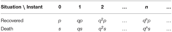
Table 1. Probabilistic model.

3.2.1. Standard Deviation

Here, we calculate the standard deviation for this probabilistic process in the number of time intervals n of infection, from the contamination until recovery or death. In order to achieve that, we have first to calculate the sum

$\begin{array}{ll}{F}_2(q)={\displaystyle \sum _{n=1}^{\infty }}{n}^2{q}^n.& (13)\end{array}$

We can calculate this sum by noting that

$\begin{array}{l}{q}^2{F}_2(q)={\displaystyle \sum _{n=2}^{\infty }}{(n-2)}^2{q}^n=F_2(q)+4{\displaystyle \sum _{n=1}^{\infty }}(1-n)q^n\\ =F_2(q)+\frac{4q}{1-q}-q-4F_1(q).\end{array}$

Hence, we find

$\begin{array}{ll}{F}_2(q)=\frac{q(1+q)}{{(1-q)}^3}.& (14)\end{array}$

We then obtain

$\overline{n^2}=(1-q)F_2(q)=\frac{q(1+q)}{{(1-q)}^2}$

and

${\overline{n}}^2=\frac{q^2}{{(1-q)}^2}.$

We can now write the standard deviation of n as

$\begin{array}{ll}\sigma =\sqrt{\overline{n^2}-{\overline{n}}^2}=\frac{\sqrt{q}}{1-q}.& (15)\end{array}$

This shows that the statistical fluctuations in the time duration of the infection as q grows to 1. By reducing q one not only decreases $\overline{n}$ but also σ.

3.3. Statistical Prediction of Active, Recovery, and Death Cases

It is very important for government officials to have estimates of the number of active (infected) cases in a given population, since these people are the ones who spread the disease. Based on knowledge of new daily infections (new confirmed cases), which we can obtain from COVID-19 databases that are updated at least every day with data from across the globe, we can make several estimates. One simple estimate of the number of active cases at time t_k is

$\begin{array}{ll}A(t_k)=C(t_k)-{R}(t_k)-D(t_k)\approx C(t_k)-C(t_k-\tau ),& (16)\end{array}$

where C(t_k) is the number confirmed cases, ${R}(t_k)$ is the number of recovered cases, D(t_k) represents the accumulated number of death cases at time t_k. Another approach is to make a statistical estimate for the number of active cases at time t_k that follows the probabilistic process described in Section 3.2, which is the following

$\begin{array}{ll}A(t_k)=-{\displaystyle \sum _{i=-1}^k}{q}^i{P}_0\Delta S(t_{k-i})={\displaystyle \sum _{i=0}^k}{q}^i\Delta C(t_{k-i}),& (17)\end{array}$

where A(t_k) = P₀I(t_k), ΔS(t_n) = S(t_n)−S(t_n−1) and, likewise, ΔC(t_n) = C(t_n)−C(t_n−1). The index k starts at 0. We also have the following probabilistic estimates for the daily increase of recovered and death cases at the k-th day

$\begin{array}{ll}\Delta {R}(t_k)={\displaystyle \sum _{i=0}^{k-1}}{q}^{i}p\Delta C(t_{k-1-i}),& (18)\end{array}$

$\begin{array}{ll}\Delta D(t_k)={\displaystyle \sum _{i=0}^{k-1}}{q}^{i}s\Delta C(t_{k-1-i}),& (19)\end{array}$

These probabilistic estimates complement the predictions from the epidemiological dynamical system model. The probabilistic aspect of the pandemic evolution can be most clearly seen when one considers short time variations, such as daily data on the number of new confirmed, recovered, or death cases. Also this allows us to make estimates of the evolution of the active, recovered, and death cases solely from the confirmed cases time series. This is most important where the recovered cases are not available or are less reliable, specially when one is counting the recovery of outpatients, since they may not take a second test to show they are actually free of the infection.

3.4. Estimates of the Parameters Used in the Model

We now make some estimates for the parameters ν, μ, ρ, and λ present in the dynamical system given in Equation (1).

3.4.1. Birth and Death Rates

In order to make our model more precise, we obtained the annual birth rate (ABR) and the annual mortality rate (AMR) from the most recently published data from Germany and from Brazil before the spread of the pandemic.

We also converted these annual rates into daily rates using the geometrical progression formulas

$\begin{array}{cc}\hfill {(1+\nu )}^{365}& =1+ABR,\hfill \\ \hfill {(1-\mu )}^{365}& =1-AMR.\hfill \end{array}$

Hence, we find the daily birth and mortality rates

$\begin{array}{l}\nu ={(1+ABR)}^{1/365}-1=e^{\frac{1}{365}\ln (1+ABR)}-1\\ \mu =1-{(1-AMR)}^{1/365}=1-e^{\frac{1}{365}\ln (1-AMR)}& (20)\end{array}$

The German data on birth and death rates were obtained from the Federal Statistical Office [28, 29]. The Brazilian data was obtained from the Brazilian Institute of Geography and Statistics (IBGE), which are from 2018. For the birth rate we divided the number of born alive infants by the population estimate for 2018 and, likewise, the number of deaths by the 2018 population estimate. The data on the born alive was collected from the site https://sidra.ibge.gov.br/tabela/2609, the number of deaths from the site https://sidra.ibge.gov.br/tabela/2654, and the population estimate from the site https://www.ibge.gov.br/estatisticas/sociais/populacao/9103-estimativas-de-populacao.html?edicao=22367&t=resultados. The birth and death rates used are shown in the Table 2 below. We provide Table 3 with information on the average total daily deaths (without the born dead) before the pandemic based on annual death rates from 2018. This should be compared with the average daily deaths due to COVID-19 as another way of assessing the severity of this pandemic.

TABLE 2

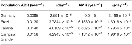
Table 2. Birth and death rates.

TABLE 3

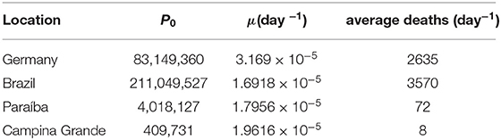
Table 3. Pre-pandemic populations and average daily deaths.

3.4.2. Contagion Rate

We use the following method to estimate the time-dependent contagion rate from the epidemiological data. From Equation (1), we can write

$\begin{array}{ll}\kappa (t)=\frac{1}{S(t)}\left[\frac{1}{I(t)}\frac{dI(t)}{dt}+\mu +\frac{1}{\tau }\right].& (21)\end{array}$

We would like to point out though, that this is not a definition of κ(t). It cannot depend on I(t), otherwise the ODE system of Equation (1) could not be integrated. This formal equation inspired us to write the following expression for the contagion rate as function of time

$\begin{array}{ll}{\kappa }_k=\kappa (t_k)\approx \frac{1}{S(t_k)}\left[\frac{1}{A(t_k)}\frac{\Delta A(t_k)}{\Delta t}+\mu +\frac{1}{\tau }\right],& (22)\end{array}$

where Δt = 1day. The daily approximation has too much fluctuation. A better approach is to replace the daily derivative by the slope of a linear regression of 7 consecutive active cases data points {A_k, A_k+1, ..., A_k+6}. One rolls this week-long window over the entire set of data points calculating κ_k. For the last 6 days of data, we use a backwards window with the data points {A_k, A_k−1, ..., A_k−6}. We chose the week interval, because all epidemiological data we have seen present weekly modulations. The most difficult part of this estimating method of κ(t) occurs at the beginning of the data sets, when the number of active cases is very small. From Equation (22), one can see that for small values of A(t_k), any errors in the derivative approximation $\frac{\Delta A(t_k)}{\Delta t}$ are amplified. Therefore, in most cases we discard the first days or weeks of epidemiological data, usually up to the day the first death occurred. In some cases, we also had to apply a cutoff to eliminate the highest values of κ(t) right at the beginning of the time series. Apart from the numerical errors described above, notice that any new imported infected case contributes strongly to the spread of the disease near the outbreak of the epidemic. Hence, at the beginning κ(t) tends to be very high. This also reflects the fact that at the start of the pandemic most populations did not keep social distancing nor used PPE such as masks.

3.4.3. Lethality and Recovery Rates

We use the following method to estimate the time-dependent lethality rate. Based on Equation (19), we can write the probability of dying for those infected with COVID-19 in a 1 day time interval as

$\begin{array}{ll}{s}_k=\frac{\Delta D(t_k)}{{\displaystyle {\sum }_{i=0}^{k-1}}{q}^i\Delta C(t_{k-1-i})}.& (23)\end{array}$

From this we obtain the daily lethality probability P_λ(k) from Equation (7). Afterwards, from Equation (12), we find the lethality rate λ_k for the k-th day. Consequently, from ρ_k + λ_k = 1/τ, we also find the recovery rate ρ_k at the k-th day. The simpler approach of estimating s_k with ΔD_k/A_k−1 introduces far more fluctuations.

3.5. Forecasting

We use a list with the last 3 weeks of κ(t) data to calculate the transition probabilities of a simple two-state Markov chain as shown in Figure 1. From this list, we obtain a list of differences Δκ_i = κ(t_i)−κ(t_i−1). Based one this, we make two probability distributions, one for increments in κ(t) and the other for decrements. If Δκ_i < 0, in the differences list, we replace it with 0, otherwise we replace it with 1. From this list of 0's and 1's, we obtain a list of lengths of the continuous sequences of 0's and 1's. We then obtain the average length of continuous stretches of 0's and 1's. We call the average length of increments of the contagion rate ${\bar{n}}_{+}$ and of decrements ${\bar{n}}_{-}$. Based on this we find the following transition probabilities

$\begin{array}{ll}\begin{array}{ccc}\hfill q_{++}& =\frac{{\bar{n}}_{+}}{1+{\bar{n}}_{+}},p_{+-}\hfill & \hfill =1-q_{++},\\ \hfill q_{--}& =\frac{{\bar{n}}_{-}}{1+{\bar{n}}_{-}},p_{-+}\hfill & \hfill =1-q_{--}.\end{array}& (24)\end{array}$

Now we use the Markov chain to decide between increasing or decreasing κ(t). The values of the increments or decrements are taken from the two probability distributions obtained as described above. We then randomly obtain predicted values of κ for 2 weeks based on a 3-week history of data. We repeat this process for 1,000 times and make an average of all these trajectories. From these trajectories we also obtain a 95% confidence interval. In the implementation of the forecasting method, we compare actual data with our predictions for the two most recent weeks. Using this same approach, we can forecast the lethality rate based on a list of daily variation of λ(t).

FIGURE 1

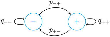
Figure 1. Markov chain diagram with transition probabilities given in Equation (24). In the − state κ(t) is decreasing in time, while in the + state, it is increasing.

4. Results and Discussion

We used the Odeint function of the Python's scientific library package SciPy [30] to integrate the ODE system of Equation (1) with the integration time-step dt = 1.0/24, which corresponds to an hour when the time unit is a day. In the cases investigated, we took τ 14 days. We chose the value that provided the best fit of the active cases with the delay estimate given in Equation (16) when the active cases data was available, such as in the cases of Germany and Brazil. When the active cases data was not available, we chose τ that would give the best fit between the theoretical prediction for the active cases and the corresponding estimate of Equation (16). We suppose this parameter does not change appreciably during the time scale of the outbreak of the pandemic until now, or at least until more efficient treatments are discovered. The initial values used are: S(0) = 1−C₀/P₀, I(0) = A₀/P₀, $R(0)={{R}}_0/P_0$, and M(0) = D₀/P₀, with P₀ being the population just before the outbreak of the pandemic, C₀ is the initial number of confirmed cases, A₀ is the initial number of active cases, ${{R}}_0$ is the initial number of recovered cases, and D₀ is the initial number of death cases, usually either 0 or 1. We now apply our model to the four cases of COVID-19 dissemination: in Germany, in Brazil, in the State of Paraíba, and in the City of Campina Grande.

In Figure 2, we show results of numerical simulation for a range of values of κ. Unlike the other results, κ is held constant during each time integration of the equations of motion given in Equation (1). This result is important in conveying the message of the paramount importance of the contagion rate on the possible outcomes of the pandemic. Not only we observe an increase in the number of deaths when the contagion rates increase, but we also see a sharp transition. When there is a growth in the contagion rate from 0.1 to 0.15, this gives rise to an extremely sharp increase in the number of deaths. This implies that there is a critical value of κ, around which there is a rapid increase in the total number of deaths due to the pandemic. Beyond the critical value, we see a saturation in the total number of deaths. The value of κ that corresponds to R₀ = 1 in our model is κ = μ+1/τ = 0.0714. We believe, this reinforces the great relevance of social distancing, since increasing the average distance between people, we will be decreasing the rate of contagion and, consequently, decreasing also the number of deaths due to COVID-19.

FIGURE 2

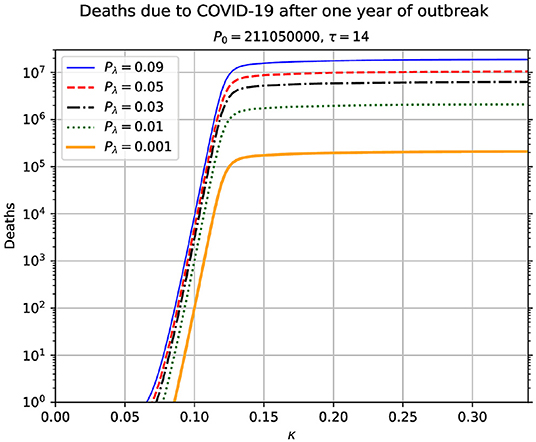
Figure 2. Total number of accumulated deaths due to the epidemic as a function of the contagion rate κ. The total time duration for each value of κ is 365 days. This result shows the high sensitivity of the model time evolution on the contagion rate. The used parameters in this simulation are indicated above the figure. In each case, it is assumed that κ remains constant during the time span of the simulation. The value of κ that corresponds to R₀ = 1 is κ^* = μ+1/τ = 0.0714.

4.1. Evolution of COVID-19 in Germany

We consider the case of Germany as a benchmark test for our epidemiological model. This is so because it is widely believed that the cases from Germany are better accounted for than in most other countries, with widespread testing of the population (https://www.labmate-online.com/news/laboratory-products/3/breaking-news/how-germany-has-led-the-way-on-covid-19-testing/52141). The initial population considered is P₀ = 83.14936 millions. The first contagion was registered on 01/27/2020 and the first death due to COVID-19 was registered on 03/09/2020. We chose this latter date as the initial point of our numerical integration.

In Figure 3A, we show the graph with the parameter estimation for the contagion rate function κ(t). At the beginning of the time series, the contagion rate is very high. To achieve the best fit between theory and the data in Figure 4, we had a cutoff at κ = 0.41, otherwise we used the estimation method described in Section 3.4.2 to obtain this time series. Note that we observe weekly modulations, likely reflecting the fact that in weekdays the contamination is higher than in weekends. The rapid decrease of κ(t) intensifies approximately around 03/22/2020, when strict social distancing rules were imposed by the German Government [18, 31]. This shows that these measures were very efficient in containing the spread of the epidemic. In Figure 4B, we show the corresponding reproduction number time series. Around April/09, the R₀(t) becomes below 1 and stays there until about June/13, when for a period of roughly 10 days it rose slightly above 1. In Figure 4C we show the time-dependent lethality and recovery probabilities, P_λ(t) and P_ρ(t), respectively. These estimates were obtained using the method described in Section 3.4.3. From early December/2020 to late March/2021, there was an increase in lethality, this might be due to the spread of COVID-19 variants, such as the alpha variant across Germany in that period. The decrease in R₀(t) from April/2021 to June/2021 is very likely due to the increased vaccination of the population. The subsequent increase in R₀(t) may be due to relaxing of preventive measures by the population and also due to spread of the delta variant.

FIGURE 3

Figure 3. Estimation of parameters of the epidemiological model applied to Germany. The initial date of the time series is the date in which the first death due to COVID-19 occurred in Germany. (A) the time variation of the contagion rate. The initial rate was very high, possibly due to exogenous cases in the early stages of the pandemic. To better fit the data with the predictions of our model we had to truncate κ(t) with values above 0.43 at the beginning of the series. (B) the reproduction number. (C) the lethality and recovery rates.

FIGURE 4

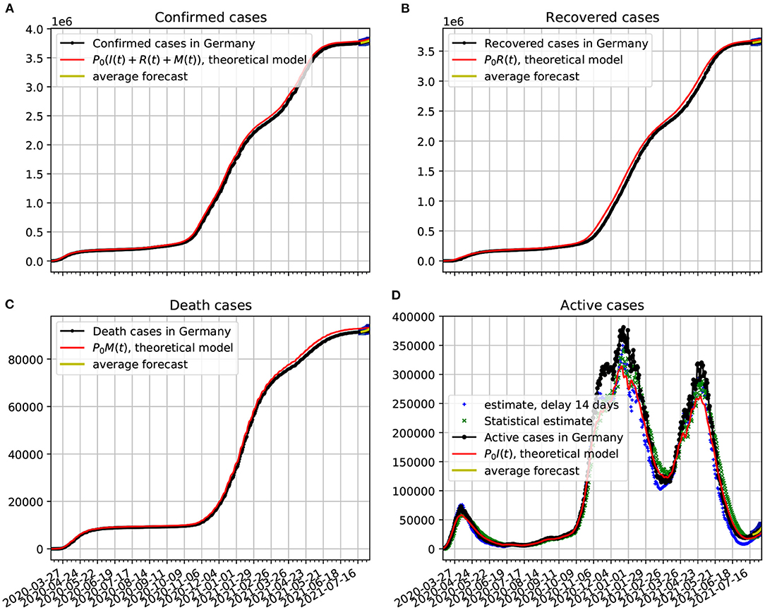
Figure 4. Comparison of epidemiological data from Germany with the best fit based on our theoretical model. Also shown near the end of the time series are the statistical forecasting 95% confidence intervals, as described in Section 3.5. The theoretical fit is obtained with τ = 14 and the parameters estimated in Figure 3. (A) Confirmed cases data from Germany compared with the theoretical prediction. (B) Recovered cases data in comparison with the theoretical prediction. (C) Death cases data compared with the theoretical prediction. (D) Active cases compared with delay estimate, statistical estimate, and the predicted theoretical curve. In all cases the functions κ(t), λ(t), and ρ(t) vary in time according to Figure 3.

In Figure 4A, we show the official data on the confirmed cases of COVID-19 plotted alongside the theoretical prediction, in which a very good agreement with the epidemiological data was obtained. The contagion rate function used is given in Figure 3. In frame Figure 4B, we plot the recovered cases data along with the theoretical predictions based on our model. In frame Figure 4C, we plot the death cases with respective theoretical curve. In frame Figure 4D, we plot the active cases data along with the theoretical predictions based on our model. The theoretical fit is not as good as in the previous figures, but it is still quite reasonable. We see a slow decline in the number of infected. Once the total number of confirmed cases basically saturates, the evolution of the active cases can be traced with a purely statistical model as the one we developed in Section 3.2. From the statistical point of view the slow decay of the active cases has to do with the large value of the dispersion in the duration of the infection, as shown in Section 3.2.1. We also plot two estimates of the active cases obtained solely from an analysis of the confirmed cases data. The delay estimate of active cases at a given time t is based on Equation 16. The statistical estimate is obtained from the probabilistic process given in Equation 17. This estimate came closer to the theoretical dynamical system model, what shows its consistency with the probabilistic model of Section 3.2. Both estimates came fairly close to the real data. Note also, that at the last 2 weeks of the time series we validate the forecasting model based on the Markov chain. Here, we show a 95% confidence band along 2 weeks. In this case the all epidemiological data fell within the predictions.

4.2. Evolution of COVID-19 in Brazil

We consider the initial time the day of the first death case in Brazil. We take Brazil's population to be approximately $P_0=211.050\times 10^6$. The initial date of the time series of the data sets used is 03/20/2020, 1 day after the first official death due to COVID-19 was recorded. We used the pre-pandemic birth and death rates shown in Table 2. The estimates of contagion, lethality and recovery rates are obtained according to the methods described in Sections 3.4.2 and 3.4.3, respectively. The time variation of the contagion rate reflects the fact that the population slowly took heed of the gravity of the pandemic and started adopting social distancing measures and using PPE.

In Figure 5A, we show the time evolution of the contagion rate κ(t). The sharp drop of this rate is likely due to the increase of isolation and social distancing that grew at the second half of March in Brazil. This is certainly due to better precautions by the population (isolation, social distancing, hand washing, and the increased use of PPE). In frame Figure 5B, we plot the reproduction number as a function of time. It is basically a scaled version of κ(t). In frame Figure 5C, we show the time evolution of the lethality and recovery probabilities, P_λ(t) and P_ρ(t), respectively. One sees more fluctuations near the beginning of the time series likely because there were less active cases then. Also, one sees that the lethality probability was very high on average in the early stages of the pandemic. This might be related with the small amount of testing in Brazil, specially in the early stages of the pandemic. Another possibility is that the medical treatment and procedures for the more severe cases of COVID-19 are being better treated since May/2020. In March/2021, there was an increase in lethality, this might be due to the gamma variants that spread from the city of Manaus across Brazil in that period.

FIGURE 5

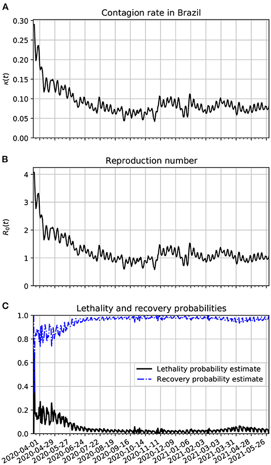
Figure 5. Estimation of the parameters of the epidemiological model applied to Brazil. (A) Time variation of the contagion rate in Brazil. This function was obtained from the statistically estimated active cases as described in Section 3.4.2. The oscillations reflect weekly variations that can be seen in the number of daily new cases. To better fit the data with the predictions of our model we had to truncate κ(t) with values above 0.29 at the beginning of the series. (B) Corresponding reproduction number evolution. (C) The lethality and recovery rates obtained with the method described in Section 3.4.3.

In Figure 6A, we compare the official data (black dotted line) of confirmed cases with the corresponding time series obtained from our proposed model (red line). In frame Figure 6B, we show a comparison between the number of recovered cases and the predicted number of recovered cases predicted by the theoretical model. The discrepancies in the fitting may have to do with delays in the confirmation of the recovered cases, as we can see in the jumps that occurred from around October/2020. One possible source of systematic error, toward sub-notification of recovered cases, could occur in mild cases, as recovered outpatients may fail to take another test to confirm their recoveries. In frame Figure 6C, we show a comparison between the number of death cases due to COVID-19 and the number of deaths predicted by the theoretical model. In frame Figure 6D, we plot the active cases data along with the theoretical predictions based on our model. The theoretical fit is not as good as in the previous figures, but it is still quite reasonable. We again validate our forecasting model with a 95% confidence interval based on Markov chain. In all cases the epidemiological data fell within the prediction range.

FIGURE 6

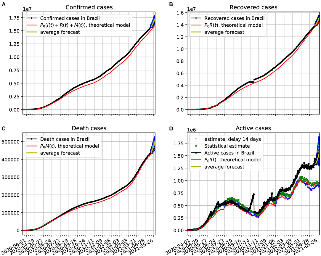
Figure 6. Comparison of epidemiological data from Brazil with the best fit based on our theoretical model. Also shown near the end of the time series are the statistical forecasting 95% confidence intervals, as described in Section 3.5. The theoretical fit is obtained with τ = 14 and the parameters estimated in Figure 5. (A) The number of official confirmed cases in Brazil compared with the theoretical prediction. (B) Time evolution of the official number of recovered cases in comparison with the theoretical prediction. (C) The number of official deaths compared with the theoretical prediction. (D) The time evolution of the official number of active cases in Brazil compared with the theoretical prediction. In all cases the functions κ(t), λ(t), and ρ(t) vary in time according to Figure 5.

4.3. Evolution of COVID-19 in Paraíba

The initial population of Paraíba is P₀ = 4, 018, 127. The first case of COVID-19 contamination was registered on 03/18/2020 and the first recorded death on 04/06/2020. We did not plot the number of recovered cases because we have not been able, so far, to obtain this data for Paraíba.

In Figure 7A, we show the time evolution of the contagion rate κ(t). Initially, the contagion rate is not as high as in Brazil's case. From about 04/06/20, the rate of contagion starts decreasing on average, although with a higher amplitude of modulation as in the case of Brazil. One sees also a decrease in the amplitude of the modulations from February to May 2021. The weekly modulations may be due to the use of public transportation during the work days of the week. In frame Figure 7B, we plot the reproduction number as a function of time. It is basically a scaled version of κ(t). In frame Figure 7C, we show the time evolution of the lethality and recovery probabilities, P_λ(t) and P_ρ(t), respectively. Again, one sees more fluctuations near the beginning of the time series likely because there were very few active cases then. Also, one sees that the lethality rate started decreasing on average after the first week of April. This might be related with the increased amount of testing in Paraíba after 2 months after the onset of the pandemic. The increase in lethality around March and April of 2021 may also be due to the spread of the gamma variants. The decreased lethality from June/2021 is likely due the vaccinations, specially of the older population.

FIGURE 7

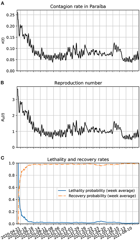
Figure 7. (A) Time variation of the contagion rate in Paraíba. This function was obtained from the statistically estimated active cases described in Section 3.3 and the method of Section 3.4.2. The initial cutoff value of κ(t) is 0.38. (B) Corresponding reproduction number evolution. (C) Estimates for the lethality and recovery rates based on Section 3.4.3.

In Figure 8A, we compare the official data (black dotted line) of confirmed cases with the corresponding time series obtained from our model (red line). In frame Figure 8B, we show a comparison between the number of death cases due to COVID-19 and the number of deaths predicted by the theoretical model. In frame Figure 8C, we show the estimated active cases. One result is based on delay and the other on the statistical method. Both methods are described in Section 3.3. We also show epidemiological model estimate (solid red line). Note also, that at the last 2 weeks of the time series we validate the forecasting model based on the Markov chain. Here, we show a 95% confidence band along 2 weeks. In this case the all epidemiological data fell well within the predictions.

FIGURE 8

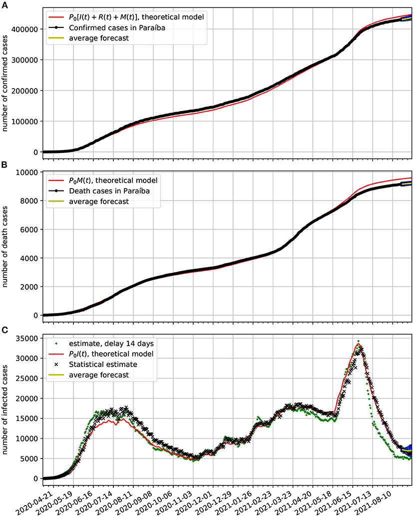
Figure 8. Comparison of epidemiological data from Paraíba with the best fit based on our theoretical model. Also shown near the end of the time series are the statistical forecasting 95% confidence intervals, as described in Section 3.5. The theoretical fit is obtained with τ = 13 and the parameters estimated in Figure 7. (A) Comparison of the number of official confirmed cases with the theoretical prediction. (B) Comparison of the number of official deaths due to COVID-19 infection with the theoretical prediction. (C) Comparison of the number of the estimated number of active cases with the theoretical prediction.

4.4. Evolution of COVID-19 in Campina Grande

The first case of COVID-19 contamination was registered on 03/27/20 and the first recorded death on 04/16/2020. We did not plot the number of recovered cases because we have not been able, so far, to obtain this data for Campina Grande.

In Figure 9A, we show the time evolution of the contagion rate κ(t). Initially, the contagion rate is not as high as in Brazil's case, but takes longer to drop. Only from about 06/07/20, the rate of contagion starts decreasing on average, although with a higher amplitude of modulation as in the case of Brazil or Paraíba. As time passes, one sees also a decrease in the amplitude of the modulations. This is certainly due to better precautions by the population (isolation, social distancing, hand washing, and the increased use of PPE). In frame Figure 9B, we plot the reproduction number as a function of time. It is basically a scaled version of κ(t). Since about the beginning of July, R₀(t) has been modulating around 1. Although, this is not enough to end the pandemic since the number of estimated active cases is still very high. In frame Figure 9C, we show the time evolution of the lethality and recovery probabilities, P_λ(t) and P_ρ(t), respectively. Again, one sees more fluctuations near the beginning of the time series likely because there were very few active cases then. Also, one sees that the lethality probability started decreasing on average after the first week of April. This might be related with the increased amount of testing in Campina Grande. The decreased lethality from June/2021 is also likely due the vaccinations, specially of the older population.

FIGURE 9

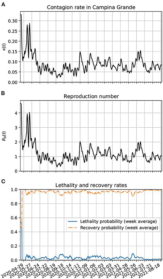
Figure 9. Parameter estimation of the theoretical model based on epidemiological data from Campina Grande. (A) Time variation of the contagion rate. This function was obtained from the statistically estimated active cases described in Section 3.3 and the method of Section 3.4.2. The initial cutoff value of κ(t) is 0.3. (B) Corresponding dynamic reproduction number evolution. (C) Estimates for the lethality and recovery rates based on Section 3.4.3.

In Figure 10A, we compare the epidemiological data (black dotted line) of confirmed cases with the corresponding time series obtained from our model (red line). In frame Figure 10B, we show a comparison between the number of death cases due to COVID-19 and the number of deaths predicted by the theoretical model. In frame Figure 10C, we show the estimated active cases. One result is based on delay (black x) and the other on the statistical method (green +). Both methods are described in Section 3.3. We also show the epidemiological model estimate (solid red line). Note also, that at the last 2 weeks of the time series we again validate the forecasting model based on the Markov chain. Here, we show a 95% confidence band along 2 weeks. In this case the all epidemiological data fell well within the predictions.

FIGURE 10

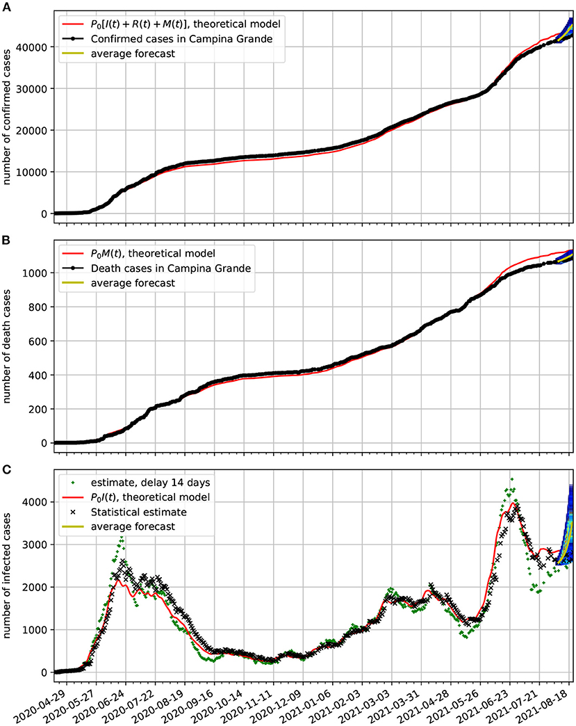
Figure 10. Comparison of epidemiological data from Campina Grande with the theoretical fit based on our model. Also shown near the end of the time series are the statistical forecasting 95% confidence intervals, as described in Section 3.5. In all cases, we used τ = 14 day and the parameters estimated in Figure 9. (A) Comparison of the number of official confirmed cases with the theoretical fit. (B) Comparison of the number of official deaths due to COVID-19 infection with the theoretical fit. (C) Comparison of the number of the estimated number of active cases with the theoretical fit.

5. Analysis of Curve Fitting of the Epidemiological Data

Although there are several papers that use root-mean-square error (RMSE) and RMSE-like measures of goodness-of-fit such as Fernandes [32], Kırbaş et al. [33], Uba et al. [34], Al-qaness et al. [35], and Gupta et al. [36], the populations are different to the ones we investigated or, as in the case of Germany, the datasets are very short compared with our datasets. The closest reference we found for comparison with our results is the work of Uba et al. [34] that only uses statistical fitting of confirmed cases data for the first 120 days of the Covid-19 epidemic in Brazil. And even then, our model is on par or better than their best fits for this time period. We also found that better measures of goodness-of-fit than RMSE are the normalized RMSE. The normalized RMSE allows comparisons of fits of different datasets and also different periods along the same dataset.

Below we provide results for the normalized RMSE, defined as

$NRMSE=\frac{RMSE}{ȳ},$

where

$RMSE=\sqrt{\frac{{\displaystyle {\sum }_{n=1}^{N_p}}{(f(t_n)-y(t_n))}^2}{N_p}},$

where N_p is the number of data points, f(t_n) is the estimate from the model, y(t_n) represents the data, and ȳ is the average of y on the same time interval of the measurement of RMSE. We show results for both the confirmed and the death cases. We used two ways to calculate the NRMSE, one is the running window NRMSE with a window length of N_w days. In the cases shown, we use N_w = 90. As a comparison, we also calculated the cumulative NRMSE starting from the first 90 days of pandemic data until a recent date.

In Figure 11, we show two different ways of measuring the NRMSE of our epidemiological data. Both the running-window and the cumulative NRMSE showed very similar results. Overall, the cumulative NRMSE values are slightly smaller for the cumulative case than the running-window case, assuming the window size of the running-window case is the initial length of the cumulative case dataset. We also notice that the cumulative case results are smoother (with broader peaks) than the running-window case. The best fitting was obtained with the data from Germany. We also notice a strong correlation between the Paraíba and Campina Grande data. This is to be unexpected because nearly the same non-farmaceutical measures were taken in both populations. In addition to that, Campina Grande is the second-largest city in Paraíba.

FIGURE 11

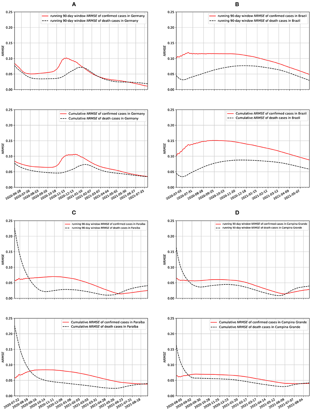
Figure 11. Running window and cumulative NRMSE data for: (A) Germany, (B) Brazil, (C) Paraíba, and (D) Campina Grande.

6. Noise in the Epidemiological Data

Here, we add noise to the epidemiological data to see if our model estimates are robust enough to the presence of uncertainties in the recording of epidemiological data. These uncertainties can arise from delays in reporting cases and also missed detection due to insufficient testing of the populations. One way to reproduce these uncertainties is to add a Gaussian noise to the epidemiological data. At each day, we add a random value obtained from a normal distribution with zero mean and standard deviation of 5% of the day's cases, which could be confirmed, death, and recovered cases. We add these statistically independent deviates to each one of these datasets, noticing that for the case of confirmed, death, and recovered cases the Gaussian deviate with zero mean and standard deviation of 5% of the day's confirmed, death, and recovered cases, respectively. From these modified epidemiological data, we obtain new time-dependent contagion, lethality, and recovery rates and integrate the equations of motion of the corresponding model. From Equation (22), we estimate that the noise effect on the contagion rate should be small. This is confirmed by our numerical results as one can see in Figure 12A, specifically in the inset.

FIGURE 12

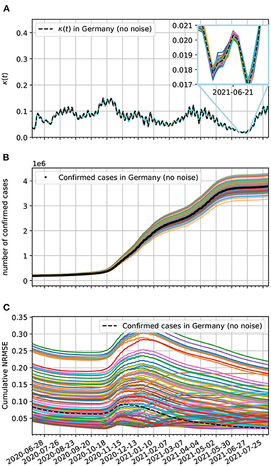
Figure 12. (A) Contagion rate estimation of the theoretical model based on epidemiological data from Germany with added noise. (B) Comparison of our theoretical model estimates with the epidemiological data from Germany. Here, the epidemiological data reporting uncertainties are accounted for by the added Gaussian noise with zero mean and a daily standard deviation of 5% on the data. All curves without labels are estimates for the epidemiological data with added Gaussian deviates. (C) Cumulative normalized NRMSE of confirmed cases with added Gaussian noise. The minimum time interval used was 90 days.

What is not usually small is the effect on the populations as can be seen in Figure 12B. In this figure, we generated 100 datasets (not plotted) with added Gaussian noise with zero mean and standard deviation on the n-th day given by σ_n = 0.05ΔC(t_n). To each of these datasets we plot the corresponding theoretical estimate (colored solid lines) For comparison, we also plot the confirmed cases data without noise (black dots).

In Figure 12C, we investigate the effect of added Gaussian noise to the curve fitting of the epidemiological data by our model via the cumulative normalized for confirmed cases. Observe that a large fraction of the time-series of the NRMSE have higher values than the the NRMSE without added noise. This likely reflects the fact that the contagion process of COVID-19 is not really random and requires contact between infected and susceptible people as assumed by compartmental epidemiological models such as the one we use. Nevertheless, even in the worst cases, the curve fitting of the data with noise is still very good, since the cumulative NRMSE is small, demonstrating that our model is robust to this sort of perturbation.

7. Conclusion

Here we summarize the main contributions of our epidemiological study of the evolution of the COVID-19 pandemic in four populations. The proposed model is an adaptation of the SIR model [4], a SIRD model [37], with some notable differences. In the SIRD model we replace the removed population by the recovered and the deceased. We allow that the contagion rate varies in time so that it reflects the fact that social distancing and isolation changes over time. We developed two ways to obtain the active population from the data on confirmed cases only. In the first approach, the number of active cases at time t is estimated simply by the difference between the confirmed population at time t minus the confirmed population at time t − τ, where τ denotes the average time span of infection. In the second approach, the number of active cases is estimated by the probabilistic model proposed here. Both approaches result in fairly accurate predictions of the active cases when the official data is available. In cases in which the data on recovered cases is not available, this approach could be the only way to estimate the number of active cases. Furthermore, we propose a simple method to track automatically the contagion rate based on the statistical estimate of active cases. We divided this data in weekly intervals and for each interval we made a linear regression to obtain the slope, and based on the equation in our model for the infected, we could obtain a daily contagion rate. This contagion rate was fed back into the equations of motion and we were able to fit the data with a minimum of or no ad hoc interventions. We noticed that the contagion rate could reach very high values at the initial stages of the spread of the epidemic in all populations investigated. This likely happens because of inherent numerical errors, as described in Section 3.4.2, and multiple infections that are imported from contaminated visitors or people returning from trips abroad. This type of dynamics is more relevant at the beginning, when the local contaminated population is small and before barriers on traveling were imposed by the governments. Here, we also take into account the contribution from the pre-pandemic birth and death rates to the evolution of the populations investigated. This could become relevant if the pandemic lasts for over a year and also it is important as a comparison for the lethality of the pandemic. According to the results exposed in the previous section, with our model we could fit the official case data from Germany, Brazil, the State of Paraíba, and city of Campina Grande quite well.

The modeling of the spread of the pandemic in Germany is very emblematic, since it clearly shows that the strict social distancing measures imposed by the government on 03/22/2020 were very effective in containing the disease, reducing the R₀(t) from 2.8 down to roughly 1 about 2 weeks later, and further down to approximately 0.5 in more 2 weeks, according to our model. The increase in lethality from December/2020 through March/2021 was probably due to the spread of COVID-19 variants, such as the alpha variant. The decrease in R₀(t) from April/2021 to June/2021 is very likely due to the increased vaccination of the population. The subsequent increase in R₀(t) may be due to relaxing of preventive measures by the population and also due to spread of the delta variant.

In the case of Brazil, we conclude that, based on the fit of the proposed model, the decrease of the reproduction number has been far more difficult and bumpier. This means the implanted social distancing measures are having an effect in thwarting the spread of the disease, but it has not been enough, since to control the pandemic R₀(t) has to remain consistently below 1 for several weeks, whereas in reality it has been oscillating around 1 for most of the time and the number of active cases is still very high. The increase in lethality after March/2021 has likely to do with the spread of gamma variants across the country.

The evolution of COVID-19 in the State of Paraíba has been similar to the national case. The amplitude of the weekly modulations of the contagion rate is considerably higher than in Brazil. This may be due to the smaller population involved. The higher lethality from February/2021 through May/2021 is probably due to the spread of the gamma variants, while the lower lethality after the last week of June/2021 is likely due to the increased anti-COVID-19 vaccination of the population. The decrease in the effective reproduction number after June/2021 may also be due to the vaccination.

As was commented in the Introduction, Campina Grande adopted a social distancing policy 1 week earlier than the report of the first confirmed case. Despite of this, the rate of contagion did not decrease as fast as it did in Germany, Brazil or Paraíba. It presents two major peaks in κ(t) spaced apart by a week since the outbreak of the disease here. Probably these could be linked to agglomeration events such as in-branch governmental relief payments to unemployed people. Also, one sees higher amplitude of the modulation of the contagion rate than in the other populations studied, this might be linked to the smaller size of the population involved. In a similar way to Paraíba, from mid June/2021 onward there is a substantial decrease in the lethality probably caused by the anti-COVID-19 vaccination campaign.

We also proposed and validated a simple forecasting method based on Markov chains and on our parameter estimation method for the evolution of the epidemiological data for up to 2 weeks. For the populations we investigated, the epidemiological data fell well within the 95% confidence interval of our predictions.

Furthermore, we calculated the NRMSE, which measures the fitting error of the differences between the epidemiological data and the estimates obtained from the evolution provided by our compartmental model with the time-dependent parameters. We use the NRMSE since it allows comparisons between curve fittings to data points at different time intervals or even between different datasets. In addition to that, we also analyzed the robusteness of our model when one introduces random errors in the epidemiological data. This mimics the fact that in real life, a fraction of the new cases of confirmed, deceased, and recovered, are reported with delays or are missed entirely.

Based on the results shown here, we conclude that the public health officials should look into the local dynamics of the spread of the disease as they compare with the theoretical predictions of models such as the one developed here. In this way, they will know where the social distancing and isolation is being more efficiently implemented. The models will be more relevant and accurate if there is more testing of the population. Even random testing should be considered, as one gains statistical information on the spread of the disease and discovers where there is more under-notification. Also, cellphone data of the motion of the population, as used by Peixoto et al. [38] and Linka et al. [19], should be considered as a means of predicting the contagion and of identifying hot spots of COVID-19. This could help identify where there are more contagions: bars, churches, supermarkets, offices, pharmacies, hospitals, bakeries, restaurants, public transportation, delivery services, or family visits, etc. Furthermore, by comparing different local strategies one could gain insight on what works better for slowing the spread of the disease. It would be interesting to see the amount of correlation in population mobility and contagion rate, this could be specially relevant at the city level. In a more refined work, one could couple several nearby cities into a network of populations.

8. Code Availability

The code used in this paper is publicly available at the gitHub repository https://github.com/aabatista/covid19_parameter_estimation. See also the Supplementary Material for a description of the code.

Data Availability Statement

All raw data supporting the conclusions of this article is publicly available. Covid-19 epidemiological data for Germany and Brazil was obtained from the site https://data.humdata.org/dataset/novel-coronavirus-2019-ncov-cases (accessed on 10/09/2021, with data collected until 09/09). The Covid-19 epidemiological data for the State of Paraíba and the City of Campina Grande was obtained from the site: https://brasil.io/dataset/covid19/files/ (accessed on 10/09/2021, with data collected until 09/09).

Author Contributions

AB designed research, developed compartmental model, statistical modeling, automated parameter estimation and forecasting, wrote and executed python code, wrote manuscript text, and made figures. SS designed research, developed compartmental model, wrote manuscript text, and wrote mathematical proofs. Both authors contributed to the article and approved the submitted version.

Conflict of Interest

The authors declare that the research was conducted in the absence of any commercial or financial relationships that could be construed as a potential conflict of interest.

Publisher's Note

All claims expressed in this article are solely those of the authors and do not necessarily represent those of their affiliated organizations, or those of the publisher, the editors and the reviewers. Any product that may be evaluated in this article, or claim that may be made by its manufacturer, is not guaranteed or endorsed by the publisher.

Acknowledgments

We would like to thank Francisco A. Brito, Antônio A. Lisboa de Souza, Michelli Barros, Joelson Campos, Pammela Queiroz, and Aldo Trajano for suggestions during the development of this work.

Supplementary Material

The Supplementary Material for this article can be found online at: https://www.frontiersin.org/articles/10.3389/fams.2022.645614/full#supplementary-material

References

1. Coronavirus disease 2019. (COVID-19) Situation Report-41 (2020). Available online at: https:www.who.int/docs/default-source/coronaviruse/situation-reports/20200301-sitrep-41-covid-19.pdf?sfvrsn=6768306d_2 (accessed on June 15, 2020).

2. Hui SD, I Azhar E, Madani TA, Ntoumi F, Kock R, Dar O, et al. The continuing 2019-nCoV epidemic threat of novel coronaviruses to global health: the latest 2019 novel coronavirus outbreak in Wuhan, China. Int J Infect Dis. (2020) 91:264–6. doi: 10.1016/j.ijid.2020.01.009

PubMed Abstract | CrossRef Full Text | Google Scholar

3. WHO. Director-General's opening remarks at the media briefing on COVID-19 - 11 March 2020 (2020). Available online at: https:www.who.int/dg/speeches/detail/who-director-general-s-opening-remarks-at-the-media-briefing-on-covid-19–11-march-2020 (accessed on May 27, 2020).

4. Kermack WO, McKendrick AG. A contribution to the mathematical theory of epidemics. Proc R Soc Lond A. (1927) 115:700–21. doi: 10.1098/rspa.1927.0118

CrossRef Full Text | Google Scholar

5. Alcaraz GG, Vargas-De-León C. Modeling control strategies for influenza A H1N1 epidemics: SIR models. Revista Mexicana de Física. (2012) 58:37–43. Available online at: https://www.redalyc.org/articulo.oa?id=57030391007

6. Bastos SB, Cajueiro DO. Modeling and forecasting the COVID-19 pandemic in Brazil. arXiv preprint arXiv:200314288. (2020) doi: 10.1038/s41598-020-76257-1

PubMed Abstract | CrossRef Full Text | Google Scholar

7. Isea R, Lonngren KE. On the mathematical interpretation of epidemics by Kermack and McKendrick. Gen Math Notes. (2013) 19:83–7. Available online at: https://www.emis.de/journals/GMN/yahoo_site_admin/assets/docs/6_GMN-3602-V19N2.32210220.pdf

PubMed Abstract | Google Scholar

8. Crokidakis N. Data analysis and modeling of the evolution of COVID-19 in Brazil. arXiv preprint arXiv:200312150. (2020).

PubMed Abstract | Google Scholar

9. Castilho C, Gondim JA, Marchesin M, Sabeti M. Assessing the efficiency of Differential control strategies for the COVID-19 epidemic. Electron J Diff Equat. (2020) 2020:1–17. Available online at: https://ejde.math.txstate.edu/Volumes/2020/64/castilho.pdf

10. Kolokolnikov T, Iron D. Law of mass action and saturation in SIR model with application to Coronavirus modelling. Infect Dis Model. (2021) 6:91–7. doi: 10.1016/j.idm.2020.11.002

PubMed Abstract | CrossRef Full Text | Google Scholar

11. Ndairou F, Area I, Nieto J, Torres DFM. Mathematical modeling of COVID-19 transmission dynamics with a case study of Wuhan. Chaos Solitons Fractals. (2020) 135:1–6. doi: 10.1016/j.chaos.2020.109846

PubMed Abstract | CrossRef Full Text | Google Scholar

12. Tang B, Wang X, Li Q, Bragazzi NL, Tang S, Xiao Y, et al. Estimation of the transmission risk of the 2019-nCoV and its implication for public health interventions. J Clin Med. (2020) 9:462. doi: 10.3390/jcm9020462

PubMed Abstract | CrossRef Full Text | Google Scholar

13. Gatto M, Bertuzzo E, Mari L, Miccoli S, Carraro L, Casagrandi R, et al. Spread and dynamics of the COVID-19 epidemic in Italy: Effects of emergency containment measures. Proc Natl Acad Sci USA. (2020) 117:10484–10491. doi: 10.1073/pnas.2004978117

PubMed Abstract | CrossRef Full Text | Google Scholar

14. Smirnova A, deCamp L, Chowell G. Forecasting epidemics through nonparametric estimation of time-dependent transmission rates using the SEIR model. Bull Math Biol. (2019) 81:4343–65. doi: 10.1007/s11538-017-0284-3

PubMed Abstract | CrossRef Full Text | Google Scholar

15. Fang Y, Nie Y, Penny M. Transmission dynamics of the COVID-19 outbreak and effectiveness of government interventions: a data driven analysis. J Med Virol. (2020) 92:645–59. doi: 10.1002/jmv.25750

PubMed Abstract | CrossRef Full Text | Google Scholar

16. Zhong L, Mu L, Li J, Wang J, Yin Z, Liu D. Early prediction of the 2019 novel coronavirus outbreak in the mainland China based on simple mathematical model. IEEE Access. (2020) 8:51761–9. doi: 10.1109/ACCESS.2020.2979599

PubMed Abstract | CrossRef Full Text | Google Scholar

17. Chen YC, Lu PE, Chang CS. A Time-dependent SIR model for COVID-19. arXiv preprint arXiv:200300122. (2020).

18. Dehning J, Zierenberg J, Spitzner FP, Wibral M, Neto JP, Wilczek M, et al. Inferring change points in the spread of COVID-19 reveals the effectiveness of interventions. Science. (2020) 369. doi: 10.1126/science.abb9789

PubMed Abstract | CrossRef Full Text | Google Scholar

19. Linka K, Goriely A, Kuhl E. Global and local mobility as a barometer for COVID-19 dynamics. Biomech Model Mechanobiol. (2021) 20:651–69. doi: 10.1007/s10237-020-01408-2

PubMed Abstract | CrossRef Full Text | Google Scholar

20. Bertozzi AL, Franco E, Mohler G, Short MB, Sledge D. The challenges of modeling and forecasting the spread of COVID-19. Proc Natl Acad Sci USA. (2020) 117:16732–16738. doi: 10.1073/pnas.2006520117

PubMed Abstract | CrossRef Full Text | Google Scholar

21. Hale JK. Ordinary Differential Equations. Dover, VA: Dover Corporation (2009).

22. Da Silva SH. Asymptotic behavior for a non-autonomous model of neural fields with variable external stimuli. J Differ Equ. (2020) 2020:1–16. Available online at: https://ejde.math.txstate.edu/Volumes/2020/92/silva.pdf

23. Diekmann O, Getto P. Boundedness, global existence and continuous dependence for nonlinear dynamical systems describing physiologically structured populations. J Diff Equat. (2005) 215:268–319. doi: 10.1016/j.jde.2004.10.025

CrossRef Full Text | Google Scholar

24. Murray JD. Mathematical Biology: I. An Introduction. vol. 17. Springer Science Business Media;. (2007).

25. Diekmann O, Heesterbeek JA, Metz JA. On the definition and the computation of the basic reproduction ratio R0 in models for infectious diseases in heterogeneous populations. J Math Biol. (1990) 28:365–82. doi: 10.1007/BF00178324

PubMed Abstract | CrossRef Full Text | Google Scholar

26. van den Driessche PJW. Reproduction numbers and sub-threshold endemic equilibria for compartmental models of disease transmission. Math Biosci. (2002) 180:29–48. doi: 10.1016/S0025-5564(02)00108-6

PubMed Abstract | CrossRef Full Text | Google Scholar

27. Ghosh S, Senapati A, Chattopadhyay J, Hens C, Ghosh D. Optimal test-kit-based intervention strategy of epidemic spreading in heterogeneous complex networks. Chaos. (2021) 31:071101. doi: 10.1063/5.0053262

PubMed Abstract | CrossRef Full Text | Google Scholar

28. Bundesamt S. Daten der Lebendgeborenen, Totgeborenen, Gestorbenen und der Gestorbenen im 1. Lebensjahr. Available online at: https:www.destatis.de/DE/Themen/Gesellschaft-Umwelt/Bevoelkerung/Geburten/Tabellen/lebendgeborene-gestorbene.html (accessed on June 15, 2020).

29. Bundesamt S. Sterbefälle und Lebenserwartung. Available online at: https:www.destatis.de/DE/Themen/Gesellschaft-Umwelt/Bevoelkerung/Sterbefaelle-Lebenserwartung/_inhalt.html;jsessionid=CE8082CB6507F3C8C4A7C93E1AEEB3FC.internet8721 (accessed on June 15, 2020).

30. Virtanen P, Gommers R, Oliphant TE, Haberland M, Reddy T, Cournapeau D, et al. SciPy 1.0: fundamental algorithms for scientific computing in python. Nat Methods. (2020) 17:261–72. doi: 10.1038/s41592-020-0772-5

PubMed Abstract | CrossRef Full Text | Google Scholar

31. Welle D. What are Germany's New Coronavirus Social Distancing Rules? (2020). Available online at: https:www.dw.com/en/what-are-germanys-new-coronavirus-social-distancing-rules/a-52881742 (accessed on July 23, 2020.).

32. Fernandes R. Compartmental epidemiological models for COVID-19: sources of uncertainty, goodness-of-fit and goodness-of-projections. IEEE Latin Am Trans. (2021) 19:1024–32. doi: 10.1109/TLA.2021.9451248

CrossRef Full Text | Google Scholar

33. Kırbaş I, Sözen A, Tuncer AD, Kazancıoğlu FŞ. Comparative analysis and forecasting of COVID-19 cases in various European countries with ARIMA, NARNN and LSTM approaches. Chaos Solitons Fractals. (2020) 138:110015. doi: 10.1016/j.chaos.2020.110015

PubMed Abstract | CrossRef Full Text | Google Scholar

34. Uba G, Yakasai H, Abubakar A, Abd Shukor MY. Predictive mathematical modelling of the total number of COVID-19 cases for Brazil. J Environ Microbiol Toxicol. (2020) 8:16–20. doi: 10.1038/s41598-021-95815-9

PubMed Abstract | CrossRef Full Text | Google Scholar

35. Al-qaness MAA, Saba AI, Elsheikh AH, Elaziz MA, Ibrahim RA, Lu S, et al. Efficient artificial intelligence forecasting models for COVID-19 outbreak in Russia and Brazil. Process Safety Environm Protect. (2021) 149:399–409. doi: 10.1016/j.psep.2020.11.007

PubMed Abstract | CrossRef Full Text | Google Scholar

36. Gupta M, Jain R, Taneja S, Chaudhary G, Khari M, Verdú E. Real-time measurement of the uncertain epidemiological appearances of COVID-19 infections. Appl Soft Comput. (2021) 101:107039. doi: 10.1016/j.asoc.2020.107039

PubMed Abstract | CrossRef Full Text | Google Scholar

37. Hethcote HW. The mathematics of infectious diseases. SIAM Rev. (2000) 42:599–653. doi: 10.1137/S0036144500371907

CrossRef Full Text | Google Scholar

38. Peixoto PS, Marcondes D, Peixoto C, Queiroz L, Gouveia R, Delgado A, et al. Potential dissemination of epidemics based on Brazilian mobile geolocation data. Part I: Population dynamics and future spreading of infection in the states of São Paulo and Rio de Janeiro during the pandemic of COVID-19. medRXiv. (2020) doi: 10.1101/2020.04.07.20056739

CrossRef Full Text | Google Scholar

Appendix

Here we summarize the proofs of proposition II.1, Proposition II.3 and Remark II.4.

A. Proof of Proposition II.1

Proof: Initially we will denote

${\kappa }_{max}=\underset{t\in [0,T]}{\sup }\kappa (t) \text{and} {\rho }_{max}=\underset{t\in [0, T]}{\sup }\rho (t)$

and we will consider ℝ⁴ with the sum norm, that is, for ξ = (S, I, R, M),

$\Vert \xi \Vert =\left|S\right|+\left|I\right|+\left|R\right|+\left|M\right|,$

where |S| ≤ S_max, |I| ≤ I_max, |R| ≤ R_max and |M| ≤ M_max.

Hence, it is easy to see that

$\begin{array}{l}|g_1(t, {\xi }_1)-g_1(t, {\xi }_2)\le |\nu -\mu \Vert S_1-S_2|+\nu |I_1-I_2|+\nu |R_1-R_2|+\kappa (t)|S_1{I}_1-S_2{I}_2|\\ \le |\nu -\mu \Vert S_1-S_2|+\nu |I_1-I_2|+\nu |R_1-R_2|+\kappa (t)|S_1\Vert I_1-I_2|\\ +\kappa (t)|I_2\Vert S_2-S_1|\\ \le |\nu -\mu \Vert S_1-S_2|+\nu |I_1-I_2|+\nu |R_1-R_2|+{\kappa }_{max}{S}_{max}|I_1-I_2|\\ +{\kappa }_{max} I_{max}|S_1-S_2|\\ \le (|\nu -\mu |+{\kappa }_{max}{I}_{max})|S_1-S_2|+(\nu +{\kappa }_{max}{S}_{max})|I_1-I_2|\\ +\nu |R_1-R_2|.\end{array}$

Hence, by writing L₁ = sup{|ν - μ| +κ_maxI_max, ν +κ_maxS_max}, we obtain

$\begin{array}{l}|g_1(t, {\xi }_1)-g_1(t, {\xi }_2)|\le L_1(|S_1-S_2|+|I_1-I_2|+|R_1-R_2|)\\ \le L_1\Vert {\xi }_1-{\xi }_2\Vert .\end{array}$

Similarly,

$\begin{array}{l}\left|g_2\right(t, {\xi }_1)-g_2(t, {\xi }_2\left)\right|\le (\mu +\frac{1}{\tau })|I_2-I_1|+\kappa \left(t\right)|S_1{I}_1-S_2{I}_2|\\ \le (\mu +\frac{1}{\tau })|I_2-I_1|+\kappa \left(t\right)|S_1\Vert I_2-I_1|+\kappa (t)|I_2\Vert S_1-S_2|\\ \le {\kappa }_{max}{I}_{max}|S_1-S_2|+{\kappa }_{max}{S}_{max}|I_1-I_2|+(\mu +\frac{1}{\tau })|I_2-I_1|;\end{array}$

thus, writing $L_2=\max \{{\kappa }_{max}{I}_{max}, {\kappa }_{max}{S}_{max}+ \mu +\frac{1}{\tau }\}$ we have

$\begin{array}{l}|g_2(t, {\xi }_1)-g_2(t,{\xi }_2)|\le L_2(|S_1-S_2|+|I_1-I_2|)\\ \le L_2\Vert {\xi }_1-{\xi }_2\Vert ;\end{array}$

$\begin{array}{l}|g_3(t, {\xi }_1)-g_3(t,{\xi }_2)|\le \rho (t)|I_1-I_2|+\mu |R_2-R_1|\\ \le {\rho }_{max}|I_1-I_2|+\mu |R_1-R_2|\\ \le L_3(|I_1-I_2|+|R_1-R_2|)\\ \le L_3\Vert {\xi }_1-{\xi }_2\Vert ,\end{array}$

where L₃ = max{ρ_max, μ} and

$|g_4(t, {\xi }_1)-g_4(t, {\xi }_2)|\le \lambda (t)|I_1-I_2|.$

Since $\frac{1}{\tau }=\rho (t)+\lambda (t)$, it follows that $\lambda (t)=\frac{1}{\tau }-\rho (t)$. Thus

${\lambda }_{max}=\underset{t\in [0,T]}{\sup }(\frac{1}{\tau }-\rho (t))<{\tau }^{-1}$

Hence,

$|g_4(t, {\xi }_1)-g_4(t, {\xi }_2)|\le \frac{1}{\tau }|I_1-I_2|\le \frac{1}{\tau }\Vert {\xi }_1-{\xi }_2\Vert .$

Therefore,

$\Vert g(t,{\xi }_1)-g(t,{\xi }_2)\Vert \le L\Vert {\xi }_1-{\xi }_2\Vert ,$

where $L=\max \{L_1,L_2,L_3, \frac{1}{\tau }\}$. This concludes the proof.

B. Proof of Proposition II.3

Proof: Define θ:[0, T] → ℝ³ by

$\theta (t)=(\kappa (t),\rho (t),\lambda (t))$

Consider the metric defined on space of the continuous functions of [0, T] in ℝ³, ℂ([0, T], ℝ³), given by

$dist(\theta ,{\theta }_0)=\underset{t\in [0,T]}{\sup }|\kappa (t)-{\kappa }_0(t)|+\underset{t\in [0,T]}{\sup }|\rho (t)-{\rho }_0(t)|+\underset{t\in [0,T]}{\sup }|\lambda (t)-{\lambda }_0(t)|.$

Now, we denote by ξ_θ(t) the solutions of Equation (1) with respect to parameter θ(t) = (κ(t), ρ(t), λ(t)) such that ξ_θ(0) = ξ₀ and we denote by ξ_θ0(t) the solutions with respect to parameter θ₀(t) = (κ₀(t), ρ₀(t), λ₀(t)) such that ξ_θ0(0) = ξ₀.

We need to show that

$\Vert {\xi }_{\theta }(t)-{\xi }_{{\theta }_0}(t)\Vert \to 0, \text{as} dist(\theta ,{\theta }_0)\to 0.$

For this, note that

$\begin{array}{ll}\Vert {\xi }_{\theta }(t)-{\xi }_{{\theta }_0}(t)\Vert \le {\displaystyle {\int }_0^t}\Vert g(s, {\xi }_{\theta }(s))-g(s, {\xi }_{{\theta }_0}(s))\Vert ds.& (25)\end{array}$

Now

$\begin{array}{l}|g_1(s, {\xi }_{\theta }(s))-g_1(s, {\xi }_{{\theta }_0}(s))|=|\nu [S(s)-S_0(s)]+\nu [I(s)-I_0(s)]+\nu [R(s)-R_0(s)]\\ +\mu [S_0(s)-S(s)]+\kappa (s)S(s)I(s)-{\kappa }_0(s)S_0(s)I_0(s)|\\ \le (\nu +\mu )|S(s)-S_0(s)|+\nu |I(s)-I_0(s)|+\nu |R(s)-R_0(s)|\\ +|\kappa (s)S(s)I(s)-{\kappa }_0(s)S(s)I(s)|\\ +|{\kappa }_0(s)S(s)I(s)-{\kappa }_0(s)S_0(s)I_0(s)|.\end{array}$

But

$|\kappa (s)S(s)I(s)-{\kappa }_0(s)S(s)I(s)|=|S(s)I(s)\Vert \kappa (s)-{\kappa }_0(s)|$

and

$\begin{array}{l}|{\kappa }_0(s)S(s)I(s)-{\kappa }_0(s)S_0(s)I_0(s)|=|{\kappa }_0(s)\Vert S(s)I(s)-S_0(s)I_0(s)|\\ \le |{\kappa }_0(s)|(|S(s)\Vert I(s)-I_0(s)|+|I_0(s)\Vert S(s)-S_0(s)|).\end{array}$

Hence,

$\begin{array}{l}|g_1(s, {\xi }_{\theta }(s))-g_1(s, {\xi }_{{\theta }_0}(s))|\%\le (\nu +\mu )|S(s)-S_0(s)|+\nu |I(s)-I_0(s)|+\nu |R(s)-R_0(s)|\\ +S_{max}{I}_{max}\underset{s\in [0,T]}{\sup }|\kappa (s)-{\kappa }_0(s)|\\ +{\kappa }_0{}_{max}(S_{max} |I(s)-I_0(s)|+I_0{}_{max}\Vert S(s)-S_0(s)|)\\ \le (\nu +\mu +{\kappa }_0{}_{max} I_0{}_{max})|S(s)-S_0(s)|\\ +(\nu +{\kappa }_0{}_{max}{S}_{max})|I(s)-I_0(s)|+\nu |R(s)-R_0(s)|\\ +S_{max}{I}_{max}dist(\theta ,{\theta }_0).\end{array}$

Thus, by writing G₁ = {ν + μ +κ_0max I_0max, ν + κ_0maxS_max}, we obtain

$\begin{array}{ll}|g_1(s, {\xi }_{\theta }(s))-g_1(s, {\xi }_{{\theta }_0}(s))|\le G_1\Vert {\xi }_{\theta }(s)-{\xi }_{{\theta }_0}(s)\Vert +S_{max}{I}_{max}dist(\theta ,{\theta }_0).& (26)\end{array}$

$\begin{array}{l}|g_2(s, {\xi }_{\theta }(s))-g_2(s, {\xi }_{{\theta }_0}(s))|=\left|\right(\mu +\frac{1}{\tau })(I_0-I)+\kappa (s)S(s)I(s)-{\kappa }_0(s)S_0(s)I_0(s)|\\ \le (\mu +\frac{1}{\tau })|I_0-I|+|S(s)I(s)\Vert \kappa (s)-{\kappa }_0(s)|\\ +|{\kappa }_0(s)\Vert S(s)I(s)-S_0(s)I_0(s)|\\ \le (\mu +\frac{1}{\tau })|I_0-I|+S_{max}{I}_{max}|\kappa (s)-{\kappa }_0(s)|\\ +{\kappa }_0{}_{max}(|S(s)\Vert I(s)-I_0(s)|+|I_0(s)\Vert S(s)-S_0(s)|)\\ \le {\kappa }_0{}_{max} I_0{}_{max}|S(s)-S_0(s)|+(\mu +\frac{1}{\tau }+{\kappa }_0{}_{max}{S}_{max})|I_0-I|\\ +S_{max}{I}_{max}dist(\theta , {\theta }_0)\\ \le G_2\Vert {\xi }_{\theta }-{\xi }_{\theta }\Vert +S_{max}{I}_{max}dist(\theta , {\theta }_0)& (27)\end{array}$

where $G_2=\max \{{\kappa }_0{}_{max} I_0{}_{max}, \mu +\frac{1}{\tau }+{\kappa }_0{}_{max}{S}_{max}\}$.

$\begin{array}{l}|g_3(s, {\xi }_{\theta }(s))-g_3(s,{\xi }_{{\theta }_0}(s))|=|\rho (s)I(s)-{\rho }_0(s)I_0(s)+\mu [R_0(s)-R(s)]|\\ \le |I(s)\Vert \rho (s)-{\rho }_0(s)|+|{\rho }_0(s)\Vert I(s)-I_0(s)|\\ +\mu [R_0(s)-R(s)]|\\ \le I_{max}\underset{s\in [0,T]}{\sup }|\rho (s)-{\rho }_0(s)|+(\underset{s\in [0,T]}{\sup }{\rho }_0(s))|I(s)-I_0(s)|\\ +\mu |R_0(s)-R(s)|\\ \le I_{max}dist(\theta ,{\theta }_0)+{\rho }_0{}_{max}|I(s)-I_0(s)|\\ +\mu |R_0(s)-R(s)|\\ \le G_3\Vert {\xi }_{\theta }(s)-{\xi }_{{\theta }_0}(s)\Vert +I_{max}dist(\theta ,{\theta }_0),& (28)\end{array}$

where G₃ = max{_ρ0max, μ}. Now,

$\begin{array}{l}|g_4(s, {\xi }_{\theta }(s))-g_4(s, {\xi }_{{\theta }_0}(s))|=|\lambda (s)I(s)-{\lambda }_0(s)I_0(s)|\\ \le |I(s)\Vert \lambda (s)-{\lambda }_0(s)|+{\lambda }_0(s)|I(s)-I_0(s)|\\ \le I_{max} (\underset{s\in [0,T]}{\sup }|\lambda (s)-{\lambda }_0(s)|)+(\frac{1}{\tau }-{\rho }_0(s)) |I(s)-I_0(s)|\\ \le \frac{1}{\tau } \Vert {\xi }_{\theta }(s)-{\xi }_{{\theta }_0}(s)\Vert +I_{max}dist(\theta ,{\theta }_0).& (29)\end{array}$

Thus, by using Equations (26), (27), (28) and (29) in (25), we find

$\begin{array}{l}\Vert {\xi }_{\theta }(t)-{\xi }_{{\theta }_0}(t)\Vert \le {\displaystyle {\int }_0^t}\{2(S_{max}{I}_{max}+I_{max})dist(\theta ,{\theta }_0)+(G_1+G_2+G_3+\frac{1}{\tau })\Vert {\xi }_{\theta }(s)-{\xi }_{{\theta }_0}(s)\Vert \}ds\\ \le 2T(S_{max}{I}_{max}+I_{max})dist(\theta ,{\theta }_0)+{\displaystyle {\int }_0^t}(G_1+G_2+G_3+\frac{1}{\tau })\Vert {\xi }_{\theta }(s)-{\xi }_{{\theta }_0}(s)\Vert ds.\end{array}$

Therefore, from Gronwall Lemma, it follows that

$\Vert {\xi }_{\theta }(t)-{\xi }_{{\theta }_0}(t)\Vert \le 2T(S_{max}{I}_{max}+I_{max})dist(\theta ,{\theta }_0)e^{(G_1+G_2+G_3+\frac{1}{\tau })T}\to 0,$

as dist(θ, θ₀) → 0.

C. Positivity of Solutions

Here we develop a constructive proof. For a more abstract alternative proof, see the supplementary material. Notice that, in the system of Equation (1), κ, ρ, and λ are non-negative continuous functions and μ and ν are positive constants. Furthermore, we have the following initial data $S(0)=1-\frac{1}{P_0}>0,I(0)=\frac{1}{P_0}>0,$ R(0) = 0 and M(0) = 0.

From the second line of the ODE system of Equation (1), we have

$I^{\prime }(t)=[-(\mu +\frac{1}{\tau })+\kappa (t)S(t)]I(t)$

Then

$\frac{I^{\prime }(t)}{I(t)}=-(\mu +\frac{1}{\tau })+\kappa (t)S(t)$

Integrating from 0 to t, we obtain

$\ln =\frac{I(t)}{I(t_0)}={\displaystyle {\int }_{t_0}^t[-\left(\mu +\frac{1}{\tau }\right)}+\kappa (s)S(s)]ds$

Thus, since I₀ > 0, we have

$\begin{array}{ll}I(t)=I_0{e}^{{\int }_{t_0}^t}{}^{[-\left(\mu +\frac{1}{\tau }\right)+\kappa (s)S(s)]ds}& (30)\end{array}$

From third equation in (1), we have

$R^{\prime }(t)+\mu R(t)=\rho (t)I(t)$

Multiplying both members of the last equation by e^μt, it follows that

$e^{\mu t}{R}^{\prime }(t)+\mu e^{\mu t}R(t)=e^{\mu t}\rho (t)I(t)$

or equivalently

$\frac{d}{dt}(e^{\mu t}R(t))=e^{\mu t}\rho (t)I(t)$

Integrating from 0 to t, we obtain

$e^{\mu t}R(t)-e^{\mu t}R(t_0)={\displaystyle {\int }_0^t{e}^{\mu s}}\rho (s)I(s)ds.$

Hence

$R(t)=e^{-\mu (t-t_0)}{R}_0+{\displaystyle {\int }_0^t{e}^{\mu s}}\rho (s)I(s)ds.$

Since R(t₀) = R₀ = 0

$\begin{array}{ll}R(t)={\displaystyle {\int }_0^t{e}^{\mu s}}\rho (s)I(s)ds>0,& (31)\end{array}$

because ρ(s) > 0 and, from (30), I > 0.

Now, from fourth equation in (1), we have

$M^{\prime }(t)=\lambda (t)I(t)$

Thus

$M(t)=M(t_0)+{\displaystyle {\int }_{t_0}^t\lambda }(s)I(s)ds$

Since M(t₀) = 0, λ > 0 and from (8), I > 0, it follows that M(t) > 0 for all t ∈ [0, T].

Finally, from first equation in (1), it follows that

$S^{\prime }(t)+(\kappa (t)I(t)+\mu -\nu )S(t)=\nu I(t)+\nu R(t)$

Let $w(t)={\int }_{t_0}^t\kappa (s)I(s)ds$ be. Then, multiplying both members by e^{w(t) + (μ-ν)t}, we obtain

$\frac{d}{dt}[e^{w(t)+(\mu -\nu )t}S(t)]=\nu (I(t)+R(t))e^{w(t)+(\mu -\nu )t}$

Integrating from 0 to t, we obtain

$e^{w(t)+(\mu -\nu )t}S(t)-e^{w(t_0)+(\mu -\nu )t_0}S(t_0)={\displaystyle {\int }_{t_0}^t{e}^{w(s)+(\mu -\nu )s}}\nu (I(s)+R(s))ds.$

Since w(t₀) = 0, it follows that

$S(t)=e^{-w(t)}{e}^{-(\mu -\nu )(t-t_0)}S(t_0)+{\displaystyle {\int }_{t_0}^t{e}^{-(w(t)-w(s))-(\mu -\nu )(t-s)}}\nu (I(s)+R(s))ds.$

As $S(t_0)=\frac{1}{P_0}>0$, ν > 0 and from (30) and (31) we have that I > 0 and R > 0, it follows that S(t) > 0 for all t ∈ [0, T].

D. Boundedness of Trajectories

If μ = ν, then, from Equation (1),

$\begin{array}{ll}\frac{d}{dt}(S+I+R+M)=0.& (32)\end{array}$

Hence, S(t) + I(t) + R(t) + M(t) = S₀+I₀+R₀+M₀ = 1. As the initial condition is S₀ = 1 - 1/P₀ and I₀ = 1/P₀, R₀ = M₀ = 0 and state variables are all non-negative, as shown above, we obtain that 0 ≤ S(t), I(t), R(t), M(t) ≤ 1. In the case of μ ≠ ν, from Equation (1), we can write

$\begin{array}{ll}\frac{d}{dt}(S+I+R+M)=(\nu -\mu )(S+I+R)\le (\nu -\mu )(S+I+R+M),& (33)\end{array}$

assuming ν > μ. Hence, we obtain S(t) + I(t) + R(t) + M(t) ≤ e^(ν-μ)t. Therefore, as S(t), I(t), R(t), and M(t) are positive, they are all bounded in any given finite time interval. If μ > ν, we obtain S(t) + I(t) + R(t) + M(t) ≤ 1.