Classification of Codimension-1 Singular Bifurcations in Low-Dimensional DAEs

1. Introduction

Differential-algebraic equations (DAEs) play an important role in dynamical system modeling such as power systems (cf. [1, 2]), nonlinear-circuits [3–7], robotics (cf. [8]), flight control systems [9], multi-body systems [10], numeric PDEs ([11] and references in Kunkel and Mehrmann [12]).

We consider quasilinear DAEs of form

$\begin{array}{ll}A(x,\alpha )\stackrel{.}{x}=f(x,\alpha ),(x,\alpha )\in {ℝ}^n\times {ℝ}^m,& (1)\end{array}$

for smooth functions A : ℝⁿ × ℝ^m → ℝ^{n × n}, f : ℝⁿ × ℝ^m → ℝⁿ of the phase variable x ∈ ℝⁿ and the parameter α ∈ ℝ^m.

In the presence of singularities, that is, points (x, α) such that det A(x, α) in Equation (1) vanishes, it is not possible to describe the local behavior of a DAE in terms of an explicit ODE. Regularization of such a singular DAE often leads to an ODE with higher dimensional manifolds of equilibria in phase space, which can manifest bifurcations without parameters (cf. [13]). System with singularities possessing the Hamiltonian structure were studied in [14–18].

In parametrized problems, a stability change due to the divergence of an eigenvalue was first analyzed by Venkatasubramanian [19, 20] and later addressed by many others [9, 20–25]. The change of stability, termed singularity-induced bifurcations (SIB), occurs when an equilibrium branch intersects a singular manifold, which results in the divergence of at least one eigenvalue through infinity.

Main efforts in studying such singularity-crossing equilibria have been given by trying to characterize the SIBs in terms of the linearized problems, such as using the matrix pencils $\left\{A(x^{*},{\alpha }^{*}),-D_{x}f(x^{*},{\alpha }^{*})\right\}$ associated to Equation (1) at the point of singularity (x^*, α^*) (cf. [20, 26]). Different sufficient conditions have been given in the framework of the tractability index (cf. [27, 28]) and the geometric index [26, 29, 30] among others. However, they may not provide a necessary and sufficient characterization of the local flow around such singularity-crossing sequilibria.

Besides SIBs, there can be other singular behavior induced by the presence of singularities such as the change of the singularity surface itself (fold) or bifurcations of singular equilibria that change significantly the dynamics near the singularity.

Quasilinear DAEs (Equation 1) have a strong connection to another important class of dynamical systems–fast-slow systems. Indeed, a system

$\epsilon \stackrel{.}{x}=f(x,y),\stackrel{.}{y}=g(x,y)$

is a fast-slow system for small ε. Setting ε to zero we obtain the so-called slow system:

$\begin{array}{ll}0=f(x,y),\stackrel{.}{y}=g(x,y),& (2)\end{array}$

in which the first equation defines the slow manifold and the second one determines the dynamics, restricted onto it. System (2) is a DAE that can be brought to the form of an ODE system via time-differentiation of the algebraic equation and the substitution of ẏ from the second one:

$\begin{array}{ll}{f}_x(x,y)\stackrel{.}{x}=-f_y(x,y)g(x,y),\stackrel{.}{y}=g(x,y).& (3)\end{array}$

That is, the slow system can be reduced to the form (Equation 1), so our research here contributes also to the studies of bifurcations in slow-fast systems (see [31]). The correspondence between the terms and notions can be viewed in the following way:

• A singularity set in DAEs corresponds to a fold set of a slow manifold;

• a fold of the singularity surface corresponds to a cusp of a slow manifold.

In this paper, we will call bifurcations that are caused by the presence of singularities singular bifurcations, which is a more general consideration of possible scenarios, which may or may not involve equilibria directly. That is, we consider bifurcations caused by singularities including SIBs but not exclusively so.

To make a clear impression of the realm of all possible bifurcations, we focus on low-dimensional quasilinear DAEs of form (Equation 1) for which x ∈ ℝ or x ∈ ℝ². Our goal is to provide a list of all possible singular bifurcations of codimension 1 in such systems.

The paper is organized as follows. In Section 2 the basic notions for the study of one-dimensional quasilinear DAEs are given, all possible codimension-one bifurcations are studied and the behavior in higher-codimension bifurcations is described. In Section 3 the main notions are given for a two-dimensional case, for which the full list of possible codimension-one bifurcations is provided. Section 4 contains the rigorous derivation of the dynamical behavior near some local singular bifurcations from Section 3.

2. Quasilinear DAEs: One-Dimensional Case

Consider a quasilinear DAE (Equation 1) for n = 1, it is given by

$\begin{array}{ll}g(x,\alpha )\stackrel{.}{x}=f(x,\alpha ),(x,\alpha )\in ℝ\times {ℝ}^m,& (4)\end{array}$

for smooth functions f : ℝ × ℝ^m → ℝ and g : ℝ × ℝ^m → ℝ. Note that in this case, the singular set is precisely the set of zeros of g given by

$\begin{array}{ll}{\Sigma }_{\alpha }=\left\{x\in ℝ:g(x,\alpha )=0\right\},& (5)\end{array}$

which under a regularity assumption on g, is composed of isolated points. We will call every such point a singularity. The set of zeros of f that are not zeros of g

$\begin{array}{ll}{E}_{\alpha }=\left\{x\in ℝ:f(x,\alpha )=0,g(x,\alpha )\ne 0\right\},& (6)\end{array}$

will be called the equilibrium set. Under a similar regularity assumption, this set is also composed of isolated points. Each such point is an equilibrium of system (Equation 4).

Definition 2.1. A point x ∈ ℝ is called a singular equilibrium if it lies in the intersection of the singular set Σ_α given by Equation (5) with the zeros set of f(x, α) for some α ∈ ℝ^m.

Definition 2.2. For a fixed parameter value α = α₀, we will call the point x₀ a simple equilibrium if it is a simple zero of f and not a zero of g:

$f(x_0,{\alpha }_0)=0,f_x^{\prime }(x_0,{\alpha }_0)\ne 0,g(x_0,{\alpha }_0)\ne 0.$

Analogously, we will call x₀ a simple singularity if it is a simple zero of g and not a zero of f:

$f(x_0,{\alpha }_0)\ne 0,g(x_0,{\alpha }_0)=0,g_x^{\prime }(x_0,{\alpha }_0)\ne 0.$

Definition 2.3. A simple singularity point x₀ is called incoming (outgoing), if there exists a small neighborhood U of x₀ such that for any initial condition x ∈ U the solution x(t) reaches x₀ in finite forward (backward) time.

Remark 2.4. The incoming or outgoing simple singularities are known in the DAE literature as the standard singular points which was introduced in [32]. They behave like an impasse point, where solutions are no longer defined being either attractive or repelling (cf. [32, 33]).

For a simple equilibrium point x₀ there exists a small neighborhood |x − x₀| < ε such that g(x, α₀) ≠ 0, and the system (Equation 4) can be rewritten as

$\begin{array}{ll}\stackrel{.}{x}=\frac{f(x,{\alpha }_0)}{g(x,{\alpha }_0)}:=\tilde{f}(x,{\alpha }_0),\text{ where }\tilde{f}(x_0,{\alpha }_0)=0.& (7)\end{array}$

Thus, the stability type of the equilibrium (x₀, α₀) is completely determined by the sign of the derivative

$\begin{array}{ll}\lambda :={\partial }_x\tilde{f}{|}_{(x_0,{\alpha }_0)}=\frac{g{\partial }_{x}f-f{\partial }_{x}g}{g^2}{|}_{(x_0,{\alpha }_0)}=\frac{{\partial }_{x}f}{g}{|}_{(x_0,{\alpha }_0)}\ne 0,& (8)\end{array}$

which is non-zero by the assumption that x₀ is a simple equilibrium for α = α₀. If λ < 0, then the equilibrium x₀ is stable; if λ > 0, then it is unstable (see Figure 1).

FIGURE 1

Figure 1. The local flow around a simple equilibrium for λ > 0 (unstable, left) and for λ < 0 (stable, right), where λ is given by Equation (8).

For a simple singularity x₀, there exists a small neighborhood in which f(x, α₀) ≠ 0 and the system (Equation 4) can be rewritten as

$\begin{array}{ll}\tilde{g}\stackrel{.}{x}=1,\text{ for }\tilde{g}=\frac{g(x,\alpha )}{f(x,\alpha )}\text{ with }\tilde{g}(x_0,{\alpha }_0)=0.& (9)\end{array}$

Thus, the following derivative

$\begin{array}{ll}\lambda ={\tilde{g}}_x{|}_{(x_0,{\alpha }_0)}=\frac{g_{x}f-g{f}_x}{f^2}{|}_{(x_0,{\alpha }_0)}=\frac{g_x}{f}{|}_{(x_0,{\alpha }_0)}\ne 0,& (10)\end{array}$

determines the type of the singularity at (x₀, α₀). More precisely, if λ > 0, then the simple singularity point x₀ is outgoing; if λ < 0, then it is incoming. See Figure 2, we put here and further below the double arrow to reflect the fact that the trajectory reaches the singularity in finite time, and the velocity grows to infinity.

FIGURE 2

Figure 2. The local flow around a simple singularity point for λ > 0 (left) and for λ < 0 (right), where λ is given by Equation (10).

It is clear from Definition 2.2, that simple equilibria and simple singularities persist under generic parametric perturbations. Indeed, the condition $f_x^{\prime }(x_0,{\alpha }_0)\ne 0$ implies that by the Implicit Function Theorem, there exists locally a unique function x^*(α) with $x^{*}({\alpha }_0)=x_0$, which fulfills the equation f(x, α) = 0. Moreover, this equilibrium maintains the same stability type, as the exponent λ in Equation (8) preserves its sign. In a similar way, one can deduct the corresponding property for a simple singularity.

Theorem 2.5. If in an open set U ⊂ ℝ system (Equation 4) possesses a finite set of equilibria and a finite set of singularities and all of them are simple, then the system is structurally stable in U.

Proof: Under sufficiently small perturbations, every simple equilibrium and every simple singularity stays in a small neighborhood of its initial position, remain simple, are distributed in the same order on the line and keep their stability types. Also, neither of these points reaches the boundary of U. The intervals bounded by these equilibria and singularities can be homeomorphically conjugated, with the direction of motion preserved.

However, when the conditions of Theorem 2.5 are violated, one may encounter bifurcations. There are three such possibilities of singular bifurcations¹:

A1. A non-simple equilibrium: f(x, α) = 0, $f_x^{\prime }(x,\alpha )=0$;

A2. A non-simple singularity: g(x, α) = 0, $g_x^{\prime }(x,\alpha )=0$;

A3. A singular equilibrium: f(x, α) = 0, g(x, α) = 0.

These cases are not exclusive to each other. They can happen simultaneously, either at the same or different points, which increases the codimension of the problem. In the following, we assume that the bifurcation conditions occur at a₀ = 0 and x₀ = 0, which can be achieved by appropriate translation of coordinates and parameters.

We start with formulating the simplest possible cases, i.e. the cases of codimension-1.

A1.1. A codimension one non-simple equilibrium: f(0, 0) = 0, $f_x^{\prime }(0,0)=0$, ${f^{″}}_x(0,0)\ne 0$, g(0, 0) ≠ 0;

A2.1. A codimension one non-simple singularity: g(0, 0) = 0, $g_x^{\prime }(0,0)=0$, ${g^{″}}_x(0,0)\ne 0$, f(0, 0) ≠ 0;

A3.0,0. A transcritical singularity (codimension-1 singular equilibrium²): f(0, 0) = 0, g(0, 0) = 0, $f_x^{\prime }(0,0)\ne 0$, $g_x^{\prime }(0,0)\ne 0$.

The case A1.1 is completely analogous to the usual fold bifurcation in dynamical systems without singularities. Indeed, since g(x, α) ≠ 0 in a small neighborhood of (x₀, α₀) = (0, 0), we can rewrite the system (Equation 4) using the function $\tilde{f}$ as defined in Equation (7), where

$\tilde{f}(0,0)={\tilde{f}}_x^{\prime }(0,0)=0,{{\tilde{f}}^{″}}_{xx}(0,0)=\frac{{f^{″}}_{xx}}{g}{|}_{(0,0)}\ne 0.$

Proposition 2.6. Assume that for system (Equation 4) the conditions of case A1.1 are fulfilled for α = 0 at x = 0, and $f_{\alpha }^{\prime }(0,0)\ne 0$. Then for all small α by an invertible change of coordinate and parameter, the system can be brought near the origin to the following normal form:

$\begin{array}{ll}\stackrel{.}{\eta }=\beta +s{\eta }^2+O({\eta }^3),& (11)\end{array}$

where $s=sign\frac{f_{xx}^{″}}{g}{|}_{(0,0)}$ (cf. Figure 3 left).

FIGURE 3

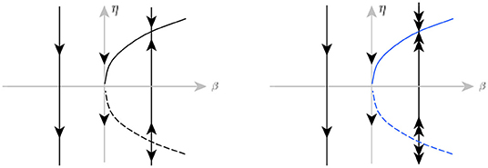
Figure 3. The equilibrium fold bifurcation (left) and the singularity fold bifurcation (right) in normal form (Equations 11, 12), respectively, where we have taken s = −1 in both cases.

This result immediately follows from Kuznetsov [34], Theorem 3.2. Similarly, one can derive the normal form for the non-simple singularity in case A2.1.

Proposition 2.7. Assume that for the system (Equation 4) the conditions of case A2.1 are fulfilled for α = 0 at x = 0, and $g_{\alpha }^{\prime }(0,0)\ne 0$. Then, for all small α by an invertible change of coordinate and parameter, the system can be brought near the origin to the following normal form:

$\begin{array}{ll}(\beta +s{\eta }^2+O({\eta }^3))\stackrel{.}{\eta }=1,& (12)\end{array}$

where $s=sign\frac{g_{xx}^{″}}{f}{|}_{(0,0)}$ (cf. Figure 3 right).

Proof: In some small neighborhood of the origin, we have f(x, α) ≠ 0 for all small α. Then, the system can be rewritten in the form (Equation 9) with

$\tilde{g}(0,0)={\tilde{g}}_x^{\prime }(0,0)=0,{{\tilde{g}}^{″}}_{xx}(0,0)=\frac{{g^{″}}_{xx}}{f}{|}_{(0,0)}\ne 0.$

We expand $\tilde{g}$ in Taylor series in x as $\tilde{g}=g_0(\alpha )+g_1(\alpha )x+g_2(\alpha )x^2+O(x^3)$ with g₀(0) = g₁(0) = 0 and g₂(0) = a ≠ 0. Using a parameter-dependent coordinate shift of the form x = y + δ(α) with δ(0) = 0, we can rewrite $\tilde{g}$ as:

$\begin{array}{l}\begin{array}{l}\tilde{g}(y+\delta (\alpha ),\alpha )=(g_0(\alpha )+g_1(\alpha )\delta (\alpha )+O({\alpha }^2))+(g_1(\alpha )\\ +2g_2(\alpha )\delta (\alpha )+O({\alpha }^2))y+(g_2(\alpha )+O(\alpha ))y^2\\ +O(y^3),\end{array}\end{array}$

where the linear term can be neglected by an appropriate choice of δ. Indeed, the coefficient of the linear term vanishes at α = δ = 0, and its derivative with respect to δ at zero is given by 2a ≠ 0. By the Implicit Function Theorem, there exists a function $\delta (\alpha )={\delta }_1\alpha +O({\alpha }^2)$ with ${\delta }_1=-\frac{g_{1,\alpha }^{\prime }(0)}{2a}$. Thus, we have

$\left[g_{0,\alpha }^{\prime }(0)\alpha +O({\alpha }^2)+a(\alpha )y^2+O(y^3)\right]\stackrel{.}{y}=1$

with a(0) = a, which becomes (12) using the scaling

$y=\frac{1}{|a(\alpha ){|}^{1/3}}\eta ,\beta =\frac{1}{|a(\alpha ){|}^{1/3}}(g_{0,\alpha }^{\prime }(0)\alpha +O({\alpha }^2)).$

Moreover, as $g_{0,\alpha }^{\prime }(0)=\frac{g_{\alpha }^{\prime }}{f}(0,0)\ne 0$, all the transformations are invertible.

The bifurcation occurs in the following way, if s = −1: for β = 0 there exists a locally unique non-simple singularity point, which disappears when β < 0 and is replaced by a pair of incoming and outgoing simple singularity points when β > 0 [see Figure 3 (right)].

The following Proposition states the normal form of the transcritical singularity bifurcation in case A3.0,0.

Proposition 2.8. If the system (Equation 4) satisfies the conditions of transcritical singularity, case A3.0.0, at (x, α) = (0, 0), and

$A:=(g_x^{\prime }{f}_{\alpha }^{\prime }-f_x^{\prime }{g}_{\alpha }^{\prime }){|}_{(0,0)}\ne 0,$

then there exists an invertible change of coordinate and parameter, which brings system (Equation 4) near the origin to the normal form

$\begin{array}{ll}\eta \stackrel{.}{\eta }=\beta +s\eta +O({\eta }^2),& (13)\end{array}$

where

$s=sign\frac{f_x^{\prime }}{g_x^{\prime }}{|}_{(0,0)}.$

(cf. Figure 4).

FIGURE 4

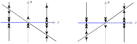
Figure 4. Transcritical singularity bifurcation of Equation (13): s > 0 (left); s < 0 (right). Both feature a transition from an incoming to an outgoing singularity as β changes from the negative to the positive, where β changes according to Equation (17). The dashed (solid) lines indicate unstable (stable) equilibrium and singularity points.

Proof: As $g_x^{\prime }(0,0)\ne 0$, the implicit equation g(x, α) = 0 can be locally uniquely resolved with respect to x for small x and α. That is, there exists a smooth function x^*(α) such that g(x^*(α), α) ≡ 0 with x^*(0) = 0 and $x^{*}(\alpha )=-\frac{g_{\alpha }^{\prime }}{g_x^{\prime }}{|}_{(0,0)}\alpha +O({\alpha }^2)$. Consider a parameter-dependent shift of coordinate x = x^*(α) + y. Then, the left-hand side of Equation (4) is transformed as

$\begin{array}{l}g(x^{*}(\alpha )+y,\alpha )=g_x^{\prime }(x^{*}(\alpha ),\alpha )y+O(y^2)=(g_1+O(\alpha ))y+O(y^2)\\ =(g_1+O(\alpha ))y(1+O(y)),& (14)\end{array}$

where $g_1=g_x^{\prime }(0,0)\ne 0$. The right-hand side function f becomes

$\begin{array}{l}f(x^{*}(\alpha )+y,\alpha )=f(x^{*}(\alpha ),\alpha )+f_x^{\prime }(x^{*}(\alpha ),\alpha )y+O(y^2)\\ =\frac{A}{g_1}\alpha +O({\alpha }^2)+(f_1+O(\alpha ))y+O(y^2),& (15)\end{array}$

where $f_1=f_x^{\prime }(0,0)$.

We choose the neighborhood small enough for term (1 + O(y)) in formula (Equation 14) to stay always positive. Then, we reparametrize time by formula dt/(1 + O(y)) = dτ, and also divide by a non-zero coefficient (g₁ + O(α)), system (Equation 4) is transformed as:

$\begin{array}{ll}y\stackrel{.}{y}=\frac{A}{g_1^2}\alpha +O({\alpha }^2)+\left(\frac{f_1}{g_1}+O(\alpha )\right)y+O(y^2).& (16)\end{array}$

It leads to Equation (13) by scaling $y\to |\frac{f_1}{g_1}+O(\alpha )|\eta$ and setting

$\begin{array}{ll}\beta =\frac{A}{f_1^2}\alpha +O({\alpha }^2).& (17)\end{array}$

Notice that as A ≠ 0, the new small parameter β diffeomorphically depends on α.

Example 2.9. The following systems demonstrate examples of cases A1.1, A2.1 and A3.0,0, respectively.

$\begin{array}{ll}(x+1)\stackrel{.}{x}=x^2+\alpha ,x,\alpha \in ℝ& (18)\end{array}$

$\begin{array}{ll}(x^2+\alpha )\stackrel{.}{x}=x+1,x,\alpha \in ℝ& (19)\end{array}$

$\begin{array}{ll}(x+x^2+\alpha )\stackrel{.}{x}=x-x^2+2\alpha ,x,\alpha \in ℝ.& (20)\end{array}$

More precisely, consider the system (Equation 18) with f(x, α) = x² + α and g(x, α) = x + 1 at (x, α) = (0, 0). It satisfies the non-simple equilibrium conditions, case A1.1:

$\begin{array}{l}f(0,0)=f_x^{\prime }(0,0)=0,{f^{″}}_{xx}(0,0)=2\ne 0,g(0,0)=1\ne 0,\\ f_{\alpha }^{\prime }(0,0)=1\ne 0.\end{array}$

By Proposition 2.6, the normal form of this bifurcation is given by Equation (11) with $s=\mathrm{\text{sign}}\frac{f_{xx}^{″}}{g}{|}_{(0,0)}=1$.

For the system (Equation 19) at the non-simple singularity point (x, α) = (0, 0), one has

$\begin{array}{l}g(0,0)=g_x^{\prime }(0,0)=0,{g^{″}}_{xx}(0,0)=2\ne 0,f(0,0)=1\ne 0,\\ g_{\alpha }^{\prime }(0,0)=1\ne 0.\end{array}$

By Proposition 2.7, the normal form here is (12) with $s=\mathrm{\text{sign}}\frac{g_{xx}^{″}}{f}{|}_{(0,0)}=1$.

The system (Equation 20) at point (x, α) = (0, 0) satisfies the conditions of the transcritical singularity:

$\begin{array}{l}f(0,0)=g(0,0)=0,f_x^{\prime }(0,0)=1\ne 0,g_x^{\prime }(0,0)=1\ne 0,\\ |\begin{array}{cc}{g}_x^{\prime }& g_{\alpha }^{\prime }\\ f_x^{\prime }& f_a^{\prime }\end{array}{|}_{(0,0)}=1\ne 0.\end{array}$

By Proposition 2.8, the normal form of this bifurcation is Equation (13) with $s=\mathrm{\text{sign}}\frac{f_x^{\prime }}{g_x^{\prime }}{|}_{(0,0)}=1$.

Besides the codimension-1 bifurcations listed by A1.1–A3.0,0, one can describe generic unfoldings of bifurcations of higher codimension in a similar way. These bifurcations admit invertible changes of coordinates (shifts), that bring them to the corresponding normal forms. We do not give a proof here, because it is straightforward: similar to cases A1.1 and A2.1 there always exists the parameter-dependent shift of coordinates x → y + δ(α) such that the term that vanishes at α = 0 and has the highest power in the Taylor expansion (y^m or yⁿ below), is eliminated for all small α. We distinguish the following bifurcations:

A1.m. A codimension-m equilibrium: f(0, 0) = 0, $f_x^{(i)}(0,0)=0$ for 1 ≤ i ≤ m and $f_x^{(m+1)}(0,0)\ne 0$, g(0, 0) ≠ 0. The normal form is:

$\begin{array}{ll}\stackrel{.}{y}={\beta }_0+{\beta }_{1}y+{\beta }_2{y}^2+\dots +{\beta }_{m-1}{y}^{m-1}+s{y}^{m+1}+O(y^{m+2})& (21)\end{array}$

A2.n. A codimension-n singularity: g(0, 0) = 0, $g_x^{(i)}(0,0)=0$ for 1 ≤ i ≤ n and $g_x^{(n+1)}(0,0)\ne 0$, f(0, 0) ≠ 0. The normal form of this bifurcation is:

$\begin{array}{ll}({\alpha }_0+{\alpha }_{1}y+{\alpha }_2{y}^2+\dots +{\alpha }_{n-1}{y}^{n-1}+s{y}^{n+1}+O(y^{n+2}))\stackrel{.}{y}=1& (22)\end{array}$

A3.m, n. A codimension-(1 + m + n) singular equilibrium: f(0, 0) = 0, $f_x^{(i)}(0,0)=0$ for 1 ≤ i ≤ m, g(0, 0) = 0, $g_x^{(j)}(0,0)=0$ for 1 ≤ j ≤ n and $f_x^{(m+1)}(0,0)\ne 0$, $g_x^{(n+1)}(0,0)\ne 0$. Its normal form is:

$\begin{array}{l}({\alpha }_0+{\alpha }_{1}y+\cdots +{\alpha }_{n-1}{y}^{n-1}+s{y}^{n+1})\stackrel{.}{y}={\beta }_0+{\beta }_{1}y+\cdots \\ +{\beta }_m{y}^m+y^{m+1}.& (23)\end{array}$

In the formulas above coefficient s is equal to either +1 or −1, and all α_i and β_i are small unfolding parameters.

Lemma 2.10. In one-dimensional system (Equation 4) the higher-order bifurcations occur in the way that under small perturbations the following dynamics is observed, depending on the case A1–A3.

Case A1.m: For any combination of integers {a₁, a₂, …, a_k}, such that $A={\displaystyle \sum _{i=1}^k}{a}_i\le m+1$ and A has the same parity with m + 1, there exists a small perturbation of normal form (21), such that it has locally k equilibria with coordinates x₁ < x₂ < … < x_k, and every x_i is simple if a_i = 1 or non-simple of codimension a_i − 1, if a_i > 1.

Case A2.n: For any combination of integers {b₁, b₂, …, b_l}, such that $B={\displaystyle \sum _{j=1}^l}{b}_i\le n+1$ and A has the same parity with n, there exists a small perturbation of normal form (22), such that it has locally l singularities with coordinates y₁ < y₂ < … < y_l, and every y_j is simple if b_j = 1 or non-simple of codimension b_j − 1, if b_j > 1.

Case A3.m, n: For any two combinations of integers {a₁, a₂, …, a_k} and {b₁, b₂, …, b_l} described above, and any two sets of local coordinates: x₁ < x₂ < … < x_k and y₁ < y₂ < … < y_l, there exists a small perturbation of normal form (23), such that it has:

1) an equilibrium at the point x_i, if x_i does not coincide with any of y_j; the equilibrium is simple if a_i = 1 or non-simple of codimension a_i − 1, if a_i > 1.

2) a singularity at the point y_j, if y_j does not coincide with any of x_i; the singularity is simple if b_j = 1 or non-simple of codimension b_j − 1, if b_j > 1.

3) a singular equilibrium at point x_i if x_i = y_j for some j; this point is degenerate of codimension a_i + b_j + 1.

Proof: First, we consider cases A1.m and A2.n. Take a set of integers {a₁, a₂, …, a_k} as described above in the respective case, and select small x₁ < x₂ < … < x_k (this means, that |x_i| < ε for some ε). Then, construct the following polynomial:

$\begin{array}{ll}P(y)={(y-x_1)}^{a_1}{(y-x_2)}^{a_2}\dots {(y-x_k)}^{a_k}.& (24)\end{array}$

It has k roots at coordinates x_i with multiplicity a_i each. If we open the parentheses in formula (24), the resulting polynomial will be a small perturbation of the order-(m + 1) polynomial standing in the right-hand side of normal form (21) or the order-(n + 1) polynomial in the left-hand side of normal form (22). The statement of Lemma on equilibria or singularities respectively, directly follows.

Now take case A3.m, n and the respective sets of integers {a₁, a₂, …, a_k} and {b₁, b₂, …, b_l} and coordinates: x₁ < x₂ < … < x_k and y₁ < y₂ < … < y_l. We construct two polynomials:

$\begin{array}{ll}\begin{array}{l}P(y)={(y-x_1)}^{a_1}{(y-x_2)}^{a_2}\dots {(y-x_k)}^{a_k},\\ Q(y)={(y-y_1)}^{b_1}{(y-y_2)}^{b_2}\dots {(y-y_l)}^{b_l}.\end{array}& (25)\end{array}$

Polynomial P(y) is the small perturbation of the right-hand side and polynomial Q(y) is the small perturbation of the left-hand side of normal form (23). At the same time, this system possesses equilibria, singularities and singular equilibria exactly as described in the Lemma.

3. Quasilinear DAEs: Two-Dimensional Case

Consider the two-dimensional quasilinear DAEs of form (Equation 1), where A is everywhere nonsingular except on the singular set Σ_α. The simplest possible form of such DAEs is given by (cf. [35])

$\begin{array}{ll}\{\begin{array}{l}g(x,y,\alpha )\stackrel{.}{x}=f_1(x,y,\alpha )\\ \stackrel{.}{y}=f_2(x,y,\alpha ),\end{array}& (26)\end{array}$

for (x, y) ∈ ℝ², α ∈ ℝ^m and g:ℝ² × ℝ^m → ℝ, $f_1,f_2:{ℝ}^2\times {ℝ}^m\to ℝ$ are smooth functions.

In this case, the singular set

$\Sigma =\left\{(x,y):g(x,y,\alpha )=0\right\}$

is the zero curve of g. This curve is the boundary of two domains:

${\Sigma }^{+}=\left\{(x,y):g(x,y,\alpha )>0\right\},{\Sigma }^{-}=\left\{(x,y):g(x,y,\alpha )<0\right\}.$

We assume that g is such that g_x has finitely many zeros on Σ. This means that ∇g is zero also at finitely many points of Σ. Every point of Σ with ∇g ≠ 0 belongs to the closure of both Σ⁺ and Σ⁻.

In order to describe the dynamics of such a two-dimensional system, we introduce the basic dynamical elements, such as special points and cycles.

Definition 3.1. A point (x, y) is called

• an equilibrium if f₁(x, y, α) = f₂(x, y, α) = 0; and g(x, y, α) ≠ 0;

• a singular equilibrium if g(x, y, α) = f₁(x, y, α) = 0.

• a fold point or a fold, if g(x, y, α) = g_x(x, y, α) = 0;

Remark 3.2. The fold points given by Definition 3.1 are also referred to as non-standard algebraic singular points in DAE terminology (cf. [32, 33]). The singular equilibria are also called as non-standard in some literature, e.g., in [32], or standard (as extended in [33]) geometric singular points.

Making time transformation $d\tau :=\frac{dt}{g}$ for g ≠ 0 in Equation (26), one obtains the desingularized system:

$\begin{array}{ll}\{\begin{array}{l}\stackrel{.}{x}=f_1(x,y,\alpha )\\ \stackrel{.}{y}=f_2(x,y,\alpha )g(x,y,\alpha ).\end{array}& (27)\end{array}$

The correspondence between the systems is the following: every trajectory Γ of system (Equation 27) contains one or more trajectories of system (Equation 26). The intersection points of Γ with singularity curve g = 0 (if any) split Γ into connected pieces Γ₁, Γ₂, … that are trajectories of Equation (26) with the same direction of time as Γ for every ${\Gamma }_i\subset {\Sigma }^{+}$ and with the opposite direction of time if ${\Gamma }_i\subset {\Sigma }^{-}$. It is clear that both equilibria and singular equilibria of system (Equation 26), given by Definition 3.1, are equilibria of the ODE system (Equation 27) in the usual sense.

Remark 3.3. Transforming the time by formula $d\tau :=\frac{dt}{-g}$ creates another desingularized system, in which the time flows in the opposite direction on every trajectory of Equation (27). The trajectories of system (Equation 26) follow the trajectories of this system in Σ⁻ and flow in the opposite direction in Σ⁺.

Consider a point M ∈ Σ and trajectory Γ ∋ M of ODE system (Equation 27), see [36] for details. The trajectory will intersect Σ transversely if it is not an equilibrium state and if its tangent vector ${(f_1,f_2·g)}^{\top }{|}_M={(f_1,0)}^{\top }$ is not orthogonal to $\nabla g={(g_x,g_y)}^{\top }$, i.e. f₁ · g_x ≠ 0. Locally, Γ is split by M into two components, Γ₁ and Γ₂ such that M = Γ(0), Γ₁ ⊂ Γ(t) for t < 0 and Γ₂ ⊂ Γ(t) for t > 0. If f₁ · g_x > 0, then Γ crosses Σ from Σ⁻ to Σ⁺, ${\Gamma }_2\subset {\Sigma }^{+}$ is the trajectory of Equation (26), and ${\Gamma }_1\subset {\Sigma }^{-}$ is the trajectory of Equation (26) with time reversal. In this case we call point M outgoing. When f₁ · g_x < 0, the direction of time is preserved on ${\Gamma }_1\subset {\Sigma }^{+}$ and reversed on ${\Gamma }_2\subset {\Sigma }^{-}$, and point M is called incoming. Inequalities f₁ · g_x > 0 and f₁ · g_x < 0 are open conditions, thus curve Σ consists of incoming Σ^inc and outgoing Σ^out zones, separated by points where f₁ · g_x = 0, those are either singular equilibria f₁ = 0 or fold points g_x = 0.

Definition 3.4. A limit cycle of system (Equation 27) is called a limit cycle of system (Equation 26), if it has no intersections with the singularity curve Σ. Otherwise, it is called a folded limit cycle.

The limit cycle is a periodic orbit of system (Equation 26). A folded limit cycle consists of more than one orbit of system (Equation 26).

3.1. Structurally Stable Objects

Definition 3.5. An equilibrium of system (Equation 26) is called simple or hyperbolic, if the linearization matrix of desingularized system (Equation 27) in this point does not have eigenvalues on the imaginary axis.

Definition 3.6. A singular equilibrium (x₀, y₀) of system (Equation 26) is called simple, if the following inequalities are fulfilled:

$\begin{array}{ll}{f}_2(x_0,y_0,\alpha )\ne 0,g_x(x_0,y_0,\alpha )\ne 0,det\frac{\partial (f_1,g)}{\partial (x,y)}{|}_{(x_0,y_0,\alpha )}\ne 0,& (28)\end{array}$

and the linearization matrix of desingularized system (Equation 27) in this point does not have eigenvalues on the imaginary axis.

Definition 3.7. A fold (x₀, y₀) of system (Equation 26) is called simple, if the following inequalities are fulfilled in it:

$\begin{array}{ll}{f}_1(x_0,y_0,\alpha )\ne 0,g_y(x_0,y_0,\alpha )\ne 0,g_{xx}(x_0,y_0,\alpha )\ne 0.& (29)\end{array}$

3.1.1. Simple Equilibria

Simple equilibria lie outside the singularity curve. A topological type of an equilibrium M is determined by eigenvalues λ₁ and λ₂ of the linearization matrix

$\begin{array}{ll}{A}_{EQ}=\left(\begin{array}{cc}{f}_{1x}& f_{1y}\\ g{f}_{2x}& g{f}_{2y}\end{array}\right).& (30)\end{array}$

For real λ₁ and λ₂, M is saddle if λ₁λ₂ < 0 and node if λ₁λ₂ > 0. If the eigenvalues are a complex-conjugate pair, the equilibrium is a focus. A node or a focus M is stable if

$\begin{array}{ll}M\in {\Sigma }^{+},Re{\lambda }_{1,2}<0\text{or}M\in {\Sigma }^{-},Re{\lambda }_{1,2}>0,& (31)\end{array}$

and unstable if

$\begin{array}{ll}M\in {\Sigma }^{+},Re{\lambda }_{1,2}>0\text{or}M\in {\Sigma }^{-},Re{\lambda }_{1,2}<0.& (32)\end{array}$

Simple equilibria persist under small perturbations, because they remain equilibria and retain their topological type in the desingularized system. Thus, in the original system, they lie outside the singularity curve Σ, and their topological type also does not change.

3.1.2. Simple Singular Equilibria

In a similar way we classify simple singular equilibria using eigenvalues λ_1,2 of linearization matrix

$\begin{array}{ll}{A}_{sEQ}=\left(\begin{array}{cc}{f}_{1x}& f_{1y}\\ g_x{f}_2& g_y{f}_2\end{array}\right).& (33)\end{array}$

Definition 3.8. Let λ_1,2 be the eigenvalues of A_sEQ in Equation (33) evaluated at a simple singular equilibrium M of Equation (26). Then, M is called a folded node, if λ_1,2 ∈ ℝ and λ₁λ₂ > 0; a folded saddle, if λ_1,2 ∈ ℝ and λ₁λ₂ < 0; and a folded focus, if λ_1,2 ∉ ℝ.

The dynamics near a folded node and a folded saddle is determined by eigendirections corresponding to eigenvalues λ_1,2 and respective invariant manifolds. The following lemma states that these eigendirections are never tangent to Σ at simple singular equilibria.

Lemma 3.9. In a folded node and a folded saddle, the eigendirections, corresponding to eigenvalues λ_1,2 are transverse to the singularity curve Σ.

Proof: We prove the lemma by contradiction. Assume that for some eigenvalue λ₁ its eigenvector is tangent to Σ. Then, tangent to Σ vector ${(g_y,-g_x)}^{\top }$ is the eigenvector of matrix A_sEQ:

$\left(\begin{array}{cc}{f}_{1x}-{\lambda }_1& f_{1y}\\ g_x{f}_2& g_y{f}_2-{\lambda }_1\end{array}\right)\left(\begin{array}{c}{g}_y\\ -g_x\end{array}\right)=\left(\begin{array}{c}{f}_{1x}{g}_y-f_{1y}{g}_x-{\lambda }_1{g}_y\\ g_x{\lambda }_1\end{array}\right)=0,$

which implies either g_x = 0 or λ₁ = 0, both conditions contradict the assumption that the considered singular equilibrium is simple.

To describe the dynamical properties of all three types of singular equilibria, we consider a small neighborhood U of M. Locally, U is divided by curve Σ into two disconnected parts given by ${\Sigma }_{loc}^{+}\subset {\Sigma }^{+}$ and ${\Sigma }_{loc}^{-}\subset {\Sigma }^{-}$.

Folded node. Consider a folded node M with λ₂ < λ₁ < 0 (for the case 0 < λ₁ < λ₂ the statement will be the same with Σ⁺ and Σ⁻ interchanged). It has a leading direction e^L defined by the eigenvector corresponding to λ₁ and a non-leading direction e^nL defined by the eigenvector corresponding to λ₂. There exists a semi-stable smooth invariant manifold W^nL(M) tangent to e^nL at point M. Its existence follows from the desingularized system (Equation 27), this system has at M a stable or a completely unstable node equilibrium, that possesses a smooth strong stable (unstable) manifold. After coming back to the original system, a part of this manifold lying in Σ⁻ changes the direction of time, so that the manifold becomes a semi-stable manifold W^nL(M).

Manifold W^nL(M) and Σ intersect transversely according to Lemma 3.9. They divide neighborhood U into four sectors, we will call them incoming, stable, outgoing and unstable. The incoming sector lies in ${\Sigma }_{loc}^{+}$ every initial condition from this sector reaches Σ^inc in forward time and leave U in backward time. The stable sector also lies in ${\Sigma }_{loc}^{+}$ and contains the leading direction e^L. The trajectories from this sector reach M tangent to e^L in forward time and reach Σ^out in backward time.

In a similar way, we describe the dynamics in ${\Sigma }_{loc}^{-}$: it is divided by W^nL(M) into unstable and outgoing sectors. In the outgoing sector trajectories leave U in forward time and reach Σ^out in backward time. In the unstable sector the trajectories reach Σ^inc in forward time and point M in backward time. All four types of behavior are illustrated at Figure 5.

FIGURE 5

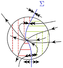
Figure 5. Dynamics around a simple singular equilibrium: the case of a folded node. The solid green and red lines mark the incoming and outgoing sectors, respectively. The dashed green and red lines mark the stable and unstable sectors, respectively.

Folded saddle. In a folded saddle M the eigenvalues of the desingularized linearization matrix are λ₁ < 0 < λ₂. Point M belongs to two smooth invariant manifolds: W⁻ tangent to eigendirection e⁻ corresponding to λ₁ and W⁺ tangent to eigendirection e⁺ corresponding to λ₂. They divide Σ⁺ into three sectors: incoming, saddle and outgoing. The incoming sector is bounded by Σ^inc and W⁻, all orbits from it reach Σ^inc in forward time and leave U in backward time. The saddle sector is bounded by W⁺ and W⁻, all orbits leave U in both directions of time. The outgoing sector is bounded by Σ^out and W⁺, the orbits in it leave U in forward time and reach Σ^out in backward time. All above describes the dynamics also in Σ⁻, where the outgoing sector is bounded by Σ^out and W⁻ and the incoming sector is bounded by Σ^inc and W⁺. The stable manifold of M is W^s(M) = M ∪ (W⁻ ∩ Σ⁺) ∪ (W⁺ ∩ Σ⁻), the unstable is W^u(M) = M ∪ (W⁺ ∩ Σ⁺) ∪ (W⁻ ∩ Σ⁻), both manifolds are C⁰ in M (see Figure 6).

FIGURE 6

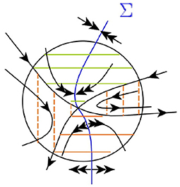
Figure 6. Dynamics around a simple singular equilibrium: the case of a folded saddle. The solid green and red lines mark the incoming and outgoing sectors, respectively. The dashed red lines mark the unstable sector.

Folded focus. Near a folded focus all orbits reach Σ^out in backward time and Σ^inc in forward time (see Figure 7).

FIGURE 7

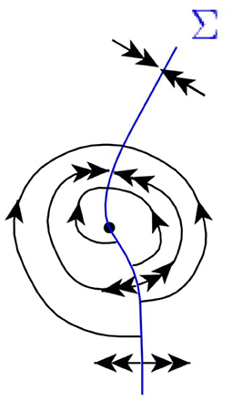
Figure 7. Dynamics around a simple singular equilibrium: the case of a folded focus.

Under small (smooth) perturbations, simple singular equilibria persist and retain their topological type. The reasons of it are that matrix (Equation 33) is non-degenerate at such point, and by the Implicit Function Theorem equation g = 0, f₁ = 0 has a unique solution for small α, provided that it exists for α = 0. Also, as the topological type of such an equilibrium persists in the desingularized system, it also persists in the original one.

3.1.3. Simple Fold

Near the simple fold point M(x₀, y₀), where (g = g_x = 0, g_xx ≠ 0, g_y ≠ 0), equation g(x, y) = 0 of the singularity curve Σ can be locally explicitly resolved as a function $y=\psi (x)=-\frac{g_{xx}(M)}{g_y(M)}{x}^2+O(x^3)$, y₀ = ψ(x₀). The fold point is a local maximum or minimum of this function. Consider the desingularized system (Equation 27) and its solution with initial condition (x₀, y₀). At the point M its y component f₂(x₀, y₀)g(x₀, y₀) vanishes, thus the trajectory is tangent to Σ, see Figure 8.

FIGURE 8

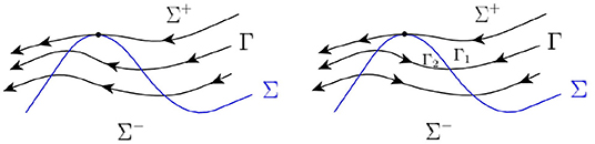
Figure 8. Left: the flow of desingularized ODE system (Equation 27); Right: the flow of the original system. The part of Γ lying in Σ⁻ reverses time. The solid points indicate simple fold points where no change of flow direction is detected.

The simple fold is either Σ⁺-convex, when g_xx(M)g_y(M) > 0 and Σ⁻-convex, when g_xx(M)g_y(M) < 0. Also, it persists under small perturbations. Indeed, for system of equations g = g_x = 0 we have

$\begin{array}{ll}\frac{\partial (g,g_x)}{\partial (x,y)}(x_0,y_0)=\left(\begin{array}{cc}0& g_y\\ g_{xx}& g_{xy}\end{array}\right)(x_0,y_0)=-g_{xx}(x_0.y_0)g_y(x_0,y_0)\ne 0& (34)\end{array}$

so that by the Implicit Function Theorem the system can be uniquely solved with respect to (x, y) for all small α. This solution gives a unique fold point in a small neighborhood of point M. In addition, condition f₁(x, y) ≠ 0 is fulfilled in some small neighborhood of the fold point, also for small α, thus no other objects (regular or singular equilibria) appear there under small perturbations.

3.1.4. Regular and Folded Limit Cycles

The limit cycles, regular and folded, both correspond to limit cycles of the desingularized system (Equation 27). By standard methods (the Poincaré crossection) one defines the multiplier μ > 0 of such an orbit. A regular cycle is simple (structurally stable), if its multiplier differs from one. A folded cycle is structurally stable also if μ ≠ 1, and, in addition, it intersects the singularity curve only transversely. The possible types of simple limit cycles are illustrated in Figure 9.

FIGURE 9

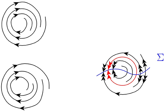
Figure 9. Dynamics around a stable limit cycle (top left), an unstable limit cycle (bottom left) and a folded limit cycle (right) of Equation (26).

3.2. Bifurcations

The bifurcations in two-dimensional DAEs are divided in three main groups: geometric (bifurcations of the singularity set), local and global bifurcations.

3.2.1. Geometric Bifurcations

Geometric bifurcations are related to the reconstruction of the topology of the singularity set Σ. It means that after arbitrary small perturbations the set Σ is topologically not equivalent to itself at the initial parameter value. This happens when its branches appear, disappear or interact with each other. Among codimension-one bifurcations, there are those, related to failure of local existence of a unique branch of Σ, i.e. existence of a point (x, y), where ∇g(x, y) = 0. At the same time, the Hessian should be non-zero at the bifurcation moment, so that the codimension is not higher than one:

$\begin{array}{ll}\nabla g(x,y)=0,det{D}^{2}g(x,y)\ne 0& (35)\end{array}$

Depending on the sign of the Hessian, two cases are possible [37]:

T1. Hyperbolic bifurcation. g_x = g_y = 0 and D²g(x, y) < 0. For example, g(x, y, α) = x² − y² − α at (0, 0, 0) (see Figure 10).

FIGURE 10

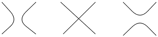
Figure 10. Hyperbolic singularity curve bifurcation of Equation (26).

T2. Elliptic bifurcation. g_x = g_y = 0 and D²g(x, y) > 0. For example, g(x, y, α) = x² + y² − α (see Figure 11).

FIGURE 11

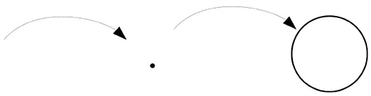
Figure 11. Elliptic singularity curve bifurcation of Equation (26).

3.2.2. Local Bifurcations

Local bifurcations occur to simple objects described in subsection 3.1, when they lose their simple properties. From the list below, bifurcations L1, L6, L8 occur outside the singularity curve Σ and thus they are unfolded as in regular ODEs. Bifurcations L2, L7, L9 involve the curve Σ, but after the desingularization procedure, they become bifurcations L1, L6, L8 respectively, in the ODE system (Equation 27) and their unfolding can be described accordingly. The rest, bifurcations L3–L5, either are unfolded in a different way in regular systems or do not have regular analogs at all. The latter are studied in detail in Section 4.

L1. Saddle-node. This bifurcation occurs when at the equilibrium point M the eigenvalues of the linearization matrix (30) are λ₁ = 0 and λ₂ ≠ 0, i.e. when f_1xf_2y − f_1yf_2x = 0. Like in a regular ODE system, a codimension-one saddle-node under small perturbations either disappears so that in some small neighborhood there are no equilibria, or splits into two simple equilibria, a saddle and a node.

L2. Singular saddle-node of type I. According to the classification by C. Kuehn [38]. This bifurcation corresponds to the existence of a singular equilibrium, for which linearization matrix (33) has eigenvalues λ₁ = 0 and λ₂ ≠ 0. This happens when f_1xg_y − f_1yg_x = 0. A codimension-one singular equilibrium of type I under small perturbations either disappears or splits into two simple singular equilibria – a folded saddle and a folded node, see Figure 12.

FIGURE 12

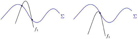
Figure 12. Singular saddle-node type 1: g = f₁ = 0, f_1xg_y − f_1yg_x = 0, g_x ≠ 0.

L3. Singular saddle-node of type II. According to the classification by C. Kuehn [38]. This bifurcation occurs when a singular equilibrium point M (f₁ = g = 0) also satisfies regular equilibrium condition f₂ = 0. A small perturbation of a codimension-one singular saddle-node of type II leads to the appearance of a simple equilibrium and a simple singular equilibrium. They appear in combinations either node + folded saddle, or saddle + folded node. For the derivation of the normal form refer to Lemma 4.1 below. The bifurcation is illustrated on Figure 13, see also [9, 20–23, 39], where such a bifurcation was studied.

FIGURE 13

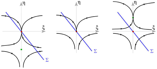
Figure 13. The singular saddle-node bifurcation of type II at (ξ^*, η^*, α^*) = (0, 0, 0) for Δ₄ > 0 and f_1x > 0. As α changes from negative to positive, the local flow changes from the left figure to right figure.

L4. Cubic fold. A fold point g = g_x = 0, g_y ≠ 0, is non-simple of codimension one (a cubic fold) if g_xx = 0 and g_xxx ≠ 0. Under small perturbations the cubic fold generically either disappears or splits into a pair of simple folds with the opposite convexity, as stated by Lemma 4.3. The bifurcation is illustrated in Figure 14.

FIGURE 14

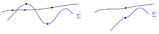
Figure 14. A cubic fold bifurcation g = g_x = g_xx = 0, f₁ ≠ 0.

L5. Singular equilibrium-fold This bifurcation occurs when at a point M both conditions of a fold and a singular equilibrium are fulfilled, i.e. g = g_x = f₁ = 0 and f₂ ≠ 0, f_1x ≠ 0, g_xx ≠ 0, g_y ≠ 0. Under small perturbations, a singular equilibrium-fold splits into a simple fold and a simple singular equilibrium, see Lemma 4.4 for details. The bifurcation is illustrated at Figure 15.

FIGURE 15

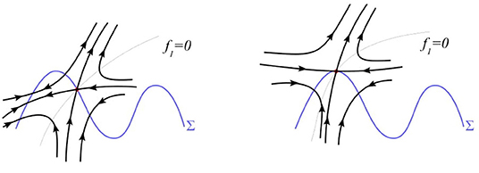
Figure 15. A singular equilibrium-fold bifurcation g = g_x = f₁ = 0, g_xx ≠ 0.

L6. Transition between folded node and folded focus. This bifurcation occurs at a singular equilibrium, when the two eigenvalues of the linearization matrix (Equation 33) coincide. In small perturbations they either become a real (folded node) or a complex-conjugated (folded focus) pair of different eigenvalues. Note that the similar transition for a regular equilibrium is not considered a bifurcation—the local flows around a node and a focus can be topologically conjugated. However, in the case of a singular equilibrium, the local flows near a folded node and a folded focus are not similar: near the folded node there exists a subset of points such that their trajectories reach the singular equilibrium in forward or backward time, while in the neighborhood of a folded focus there are no such orbits (see Subsection 3.1.2 for details).

L7. Andronov-Hopf bifurcation. This standard bifurcation occurs when a stable (unstable) focus equilibrium has a pair of pure imaginary eigenvalues (of matrix Equation 30). Under small perturbations such a weak focus either becomes a simple stable (unstable) focus, or unstable (stable) focus and a stable (unstable) limit cycle is born.

L8. Folded Andronov-Hopf bifurcation. This bifurcartion takes place, when linearisation matrix (Equation 33) has a pair of pure imaginary eigenvalues [40]. This bifurcation corresponds to a regular Andronov-Hopf in the desingularized system (Equation 27), in which a limit cycle is born from a focus equilibrium. In the original system (Equation 26) under small perturbations a folded limit cycle is born from a folded focus.

L9. Double limit cycle. Existence of a limit cycle with multiplier equal to +1. Under small perturbations this cycle either disappears or is split into stable and unstable simple limit cycles, see Figure 16.

FIGURE 16

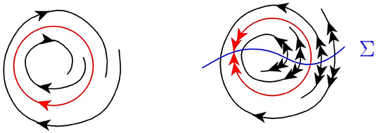
Figure 16. Dynamics around a double limit cycle (left) and a folded double limit cycle (right) of Equation (26).

L10. Folded double limit cycle. This bifurcation corresponds to the existence of a double limit cycle in the desingularized system (Equation 27), that intersects the singularity curve. Under small perturbations such a cycle either disappears or is split into a pair of simple folded limit cycles.

3.2.3. Global Bifurcations

This is the class of bifurcations, in which special orbits (homoclinic or heteroclinic) exist in the system. They are usually destroyed by small perturbations. Such orbits can be regular, when they have no intersections with the singularity curve Σ, or folded if such an intersection point exist.

G1. A homoclinic orbit to a saddle. In the desingularized system (Equation 27) there exists a homoclinic loop Γ to a saddle equilibrium, that is also an equilibrium in system (Equation 26).

G1a. Regular. This is the standard homoclinic bifurcation, when the image of Γ does not intersect Σ. Upon small perturbations it either just disappears, or disappears with the creation of a limit cycle.

G1b. Folded. The image of Γ in Equation (26) has intersections with Σ. Under small pertubations, such a homoclinic loop gives rise to a folded limit cycle.

G2. A homoclinic orbit to a folded saddle a homoclinic orbit Γ exists in the desingularized system (Equation 27). In the original system (Equation 26) this equilibrium lies at Σ.

G2a. Regular. In the original system (Equation 26) the image of Γ does not intersect Σ. Under small perturbations, when the folded saddle disappears, a regular limit cycle is born.

G2b. Folded. In the original system (Equation 26) the image of Γ has intersections with Σ. Under small perturbations, when the folded saddle disappears, a folded limit cycle is born.

G3. A homoclinic orbit to a fold point. In the desingularized system (Equation 27) there exists a simple limit cycle L. In the original system (Equation 26) the image of curve L is tangent to Σ at a simple fold point F.

G3a. Regular. The image of curve L does not have common points with Σ other than F. Under small perturbations, cycle L in system (Equation 27) persists, and in system (Equation 26) this curve becomes either a regular or a folded limit cycle.

G3b. Folded. The image of curve L have intersections with Σ other than F. Under small perturbations, cycle L in system (Equation 27) persists, and in system (Equation 26) it becomes a folded limit cycle.

G4. A homoclinic orbit to a saddle-node. In the desingularized system (Equation 27) there exists a homoclinic orbit L to a saddle-node equilibrium M. In system (Equation 26) point M does not belong to singularity curve Σ. Upon the disappearance of the equilibrium a limit cycle is born in system (Equation 27).

G4a. Regular. The image of L in system (Equation 26) does not intersect the singularity curve Σ. Upon the disappearance of the equilibrium a limit cycle is born also in the original system (Equation 26).

G4b. Folded. The image of L in system (Equation 26) intersects transversely the singularity curve Σ. Upon the disappearance of the equilibrium a folded limit cycle is born.

G5. A homoclinic orbit to a singular saddle-node of type I. In the desingularized system (Equation 27) there exists a homoclinic orbit L to a saddle-node equilibrium M. In system (Equation 26) point M is a singular equlibrium (a singular saddle-node of type I). Upon the disappearance of the equilibrium a periodic orbit is born in system (Equation 27).

G5a. Regular. The image of L in system (Equation 26) does not intersect the singularity curve Σ. Upon the disappearance of the singular equilibrium a limit cycle is born in the original system (Equation 26).

G5b. Folded. The image of L in system (Equation 26) intersects transversely the singularity curve Σ. Upon the disappearance of the singular equilibrium a folded limit cycle is born.

G6. A heteroclinic connection. This bifurcation corresponds to the existence of such an orbit L in system (Equation 27) that

• passes through two different fold points of system (Equation 26). In system (Equation 26) a piece of L that lies between the fold points, is a heteroclinic connection of two folds (see Figure 17).

• passes through one fold point F of system (Equation 26) and tends to an equilibrium in forward or backward time, without passing through other fold points that differ from F. This is a heteroclinic connection of a fold and a regular or singular equilibrium in system (Equation 26)

• tends to different equilibria in both forward and backward time, without passing through any of folds of system (Equation 26). This is a heteroclinic connection between two equilibria, two singular equilibria or between an equilibrium and a singular equilibrium.

FIGURE 17

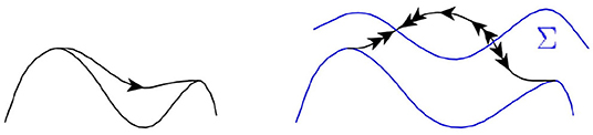
Figure 17. Dynamics around a regular heteroclinic connection (left) and a folded heteroclinic connection (right) of Equation (26).

All the heteroclinic connections listed above can be either regular, when they do not intersect the singularity curve, or folded, when such an intersection exists. Under small perturbations heteroclinic connections are generically broken.

4. Local Bifurcations L3–L5

In this section the character of those local bifurcations, that do not have analogs in regular ODEs is studied in detail. These bifurcations are L3: Singular saddle-node of type II, L4: Cubic fold and L5: Singular equilibrium-fold from subsection 3.2.2.

We introduce the following notations:

$\begin{array}{ll}\begin{array}{c}{\Delta }_1=det\frac{\partial (f_1,f_2)}{\partial (x,y)}{|}_{(0,0,0)},{\Delta }_2=det\frac{\partial (f_1,g)}{\partial (x,y)}{|}_{(0,0,0)},\\ {\Delta }_3=det\frac{\partial (g,g_x)}{\partial (y,\alpha )}{|}_{(0,0,0)},{\Delta }_4=\frac{\partial (f_1,f_2,g)}{\partial (x,y,\alpha )}{|}_{(0,0,0)},\\ {\Delta }_5=\frac{\partial (f_1,g,g_x)}{\partial (x,y,\alpha )}{|}_{(0,0,0)}.\end{array}& (36)\end{array}$

4.1. L3: Singular Saddle-Node of Type II

This bifurcation occurs at point M(0, 0) when both conditions for an equilibrium and a singular equilibrium are fulfilled in it for α = 0. This means that g(0, 0, 0) = f₁(0, 0, 0) = f₂(0, 0, 0) = 0. We assume that the following inequalities also hold, so that the codimension is equal to one and that the parametric family is transversal:

$\begin{array}{ll}\begin{array}{c}{f}_{1x}(0,0,0)\ne 0,g_x(0,0,0)\ne 0,{\Delta }_1\ne 0,{\Delta }_2\ne 0,{\Delta }_4\ne 0.\end{array}& (37)\end{array}$

Lemma 4.1. Assume that genericity (codimension one + transversality) conditions (37) are fulfilled at a singular saddle-node type II point M. Then in a generic unfolding point M splits into a pair of structurally stable points, a regular and a singular equilibria. They are either a saddle and a folded node or a node and a folded saddle.

Proof: First of all, we note that equations f₁ = f₂ = g = 0 have a solution x = y = α = 0, and by the transversality condition Δ₄ ≠ 0 no other solution exists nearby, thus for small α ≠ 0 no other singular saddle-nodes of type II exist in some small neighborhood of the origin.

Condition Δ₁ ≠ 0 implies that for all small α equations f₁ = f₂ = 0 have a unique equilibrium solution

$\begin{array}{l}(x_e(\alpha ),y_e(\alpha ))=\frac{1}{{\Delta }_1}\left(det\frac{\partial (f_1,f_2)}{\partial (y,\alpha )}{|}_{(0,0,0)},-det\frac{\partial (f_1,f_2)}{\partial (x,\alpha )}{|}_{(0,0,0)}\right)\alpha \\ +O({\alpha }^2).& (38)\end{array}$

Similarly, as Δ₂ ≠ 0, equations f₁ = g = 0 have a unique singular equilibrium solution:

$\begin{array}{l}(x_s(\alpha ),y_s(\alpha ))=\frac{1}{{\Delta }_2}\left(det\frac{\partial (f_1,g)}{\partial (y,\alpha )}{|}_{(0,0,0)},-det\frac{\partial (f_1,g)}{\partial (x,\alpha )}{|}_{(0,0,0)}\right)\alpha \\ +O({\alpha }^2).& (39)\end{array}$

At the bifurcation moment α = 0 the linearization matrix (33) at the singular saddle node has eigenvalues λ₁ = f_1x ≠ 0 and λ₂ = 0. Upon a small perturbation, linearization matrices (30) and (33) of, respectively, the equilibrium and the singular equilibrium, will have real eigenvalues λ₁ = f_1x(0, 0, 0) + O(α) and λ₂ = O(α), so they have either node or saddle type. The sign of the first eigenvalue at each point is given for small α by the sign of derivative f_1x(0, 0, 0). The product of eigenvalues is equal to the determinant of the linearization matrix. At the equilibrium the determinant is:

$det{A}_{EQ}=g(x^e(\alpha ),y^e(\alpha ),\alpha )({\Delta }_1+O(\alpha ))={\Delta }_4\alpha +O({\alpha }^2),$

and at the singular equilibrium:

$det{A}_{sEQ}=f_2(x^s(\alpha ),y^s(\alpha ),\alpha )({\Delta }_2+O(\alpha ))=-{\Delta }_4\alpha +O({\alpha }^2).$

Thus, the bifurcation occurs in the following way:

When Δ₄α > 0, the equilibrium is a node (stable if f_1x < 0 and unstable if f_1x > 0), and the singular equilibrium is a folded saddle;

When Δ₄α < 0, the equilibrium is a saddle, and the singular equilibrium is a folded node.

Example 4.2. Consider

$\begin{array}{ll}\{\begin{array}{l}(x-x^3)\stackrel{.}{x}=y-x+\alpha \\ \stackrel{.}{y}=y\end{array}.& (40)\end{array}$

Then, for α = 0 we have f₁ = f₂ = g = 0, i.e. a singular saddle-node of type II at the origin (x, y) = (0, 0). By formulas (36), it follows that f_1x = −1, g_x = 1, Δ₁ = −1, Δ₂ = −1 and Δ₄ = −1, the conditions (37) are fulfilled. For small α this bifurcation point unfolds into an equilibrium EQ: (x^e, y^e) = (α, 0) + O(α²) and a singular equilibrium sEQ: (x^s, y^s) = (0, −α) + O(α²). For α > 0 EQ is a stable node and sEQ is a folded saddle. For α < 0, EQ is a saddle and sEQ is a folded node.

4.2. L4: Cubic Fold

The cubic fold bifurcation occurs at point M(0, 0) for α = 0 if conditions g = g_x = g_xx = 0 are fulfilled at it. In addition, to keep the codimension of the problem equal to one and to construct a transversal parametric family, we assume the following inequalities to hold:

$\begin{array}{ll}{f}_1\ne 0,g_y\ne 0,g_{xxx}\ne 0,{\Delta }_3\ne 0& (41)\end{array}$

Lemma 4.3. Assume that genericity (codimension one + transversality) conditions (Equation 41) are fulfilled at a cubic fold point M. Then in a generic unfolding point M splits into a pair of simple folds, or disappears.

Proof: For system of equations g = g_x = 0 the Implicit Function Theorem are not fulfilled, because $\frac{\partial (g,g_x)}{\partial (x,y)}{|}_{(0,0,0)}=0$. Then we look for a solution of this system in the form

$x={\beta }_1{\alpha }^{{\delta }_1}+o({\alpha }^{{\delta }_1}),y={\beta }_2{\alpha }^{{\delta }_2}+o({\alpha }^{{\delta }_2})$

for positive α, and

$x={\beta }_1{(-\alpha )}^{{\delta }_1}+o({(-\alpha )}^{{\delta }_1}),y={\beta }_2{(-\alpha )}^{{\delta }_2}+o({(-\alpha )}^{{\delta }_2})$

for negative α. The equations take form

$\begin{array}{ll}\begin{array}{l}0=g_y{\beta }_2{\alpha }^{{\delta }_2}+g_{\alpha }\alpha +\frac{1}{6}{g}_{xxx}{\beta }_1^3{\alpha }^{3{\delta }_1}+h.o.t.\\ 0=g_{xy}{\beta }_2{\alpha }^{{\delta }_2}+g_{x\alpha }\alpha +\frac{1}{2}{g}_{xxx}{\beta }_1^2{\alpha }^{2{\delta }_1}+h.o.t.\end{array}& (42)\end{array}$

and respectively

$\begin{array}{ll}\begin{array}{l}0=g_y{\beta }_2{(-\alpha )}^{{\delta }_2}-g_{\alpha }(-\alpha )+\frac{1}{6}{g}_{xxx}{\beta }_1^3{(-\alpha )}^{3{\delta }_1}+h.o.t.\\ 0=g_{xy}{\beta }_2{(-\alpha )}^{{\delta }_2}-g_{x\alpha }(-\alpha )+\frac{1}{2}{g}_{xxx}{\beta }_1^2{(-\alpha )}^{2{\delta }_1}+h.o.t.\end{array}& (43)\end{array}$

For them to be solvable it is required that δ₁ = 1/2, δ₂ = 1. Then for α > 0 from (42) we have

$\begin{array}{ll}{\beta }_1^2=\frac{2{\Delta }_3}{g_y{g}_{xxx}},{\beta }_2=-\frac{g_{\alpha }}{g_y}& (44)\end{array}$

and for α < 0 from (43):

$\begin{array}{ll}{\beta }_1^2=-\frac{2{\Delta }_3}{g_y{g}_{xxx}},{\beta }_2=\frac{g_{\alpha }}{g_y}.& (45)\end{array}$

Then, two simple folds exist for perturbations $\frac{2{\Delta }_3}{g_y{g}_{xxx}}\alpha >0$, and the cubic fold disappears, and no folds exist locally, when $\frac{2{\Delta }_3}{g_y{g}_{xxx}}\alpha <0$.

4.3. L5. Singular Equilibrium-Fold

The singular equilibrium-fold bifurcation occurs at point M(0, 0) for α = 0 if conditions g = g_x = f₁ = 0 are fulfilled at it. In addition, to keep the codimension of the problem equal to one and to construct a transversal parametric family, we assume the following inequalities to hold:

$\begin{array}{ll}{g}_y\ne 0,g_{xx}\ne 0,{\Delta }_2\ne 0,{\Delta }_3\ne 0,{\Delta }_5\ne 0& (46)\end{array}$

Lemma 4.4. Assume that genericity (codimension one + transversality) conditions (Equation 46) are fulfilled at a singular equilibrium-fold point M. Then in a generic unfolding point M splits into a simple folds and a simple singular equilibrium.

Proof: By the transversality condition Δ₅ ≠ 0, system of equations g = g_x = f₁ = 0 has locally no solutions for α ≠ 0, then the singular equilibrium-fold disappears under such small perturbations.

The genericity condition Δ₂ ≠ 0 implies that system of equations f₁ = g = 0 has locally a unique singular equilibrium solution for small α:

$\begin{array}{l}(x_s(\alpha ),y_s(\alpha ))=\frac{1}{{\Delta }_2}\left(det\frac{\partial (f_1,g)}{\partial (y,\alpha )}{|}_{(0,0,0)},-det\frac{\partial (f_1,g)}{\partial (x,\alpha )}{|}_{(0,0,0)}\right)\alpha \\ +O({\alpha }^2).& (47)\end{array}$

Also, the genericity condition Δ₃ ≠ 0 implies that a unique fold solution of system g = g_x = 0 exists for small α:

$\begin{array}{l}(x_f(\alpha ),y_f(\alpha ))=\frac{1}{{\Delta }_3}\left(det\frac{\partial (g,g_x)}{\partial (y,\alpha )}{|}_{(0,0,0)},-det\frac{\partial (g,g_x)}{\partial (x,\alpha )}{|}_{(0,0,0)}\right)\\ \alpha +O({\alpha }^2).& (48)\end{array}$

Data Availability Statement

The original contributions presented in the study are included in the article/supplementary material, further inquiries can be directed to the corresponding author.

Author Contributions

HR wrote the Introduction section, prepared the figures and the examples. IO contributed to the basic definitions and explanation of the dynamics, as well as the preparation of the list of bifurcations. Both authors contributed to the conception, design of the study, computation of the normal forms, manuscript revisions, read, and approved the submitted version.

Funding

This article is a contribution to the project M7 (Dynamics of Geophysical Problems in Turbulent Regimes) of the Collaborative Research Centre TRR 181 Energy Transfer in Atmosphere and Ocean funded by the Deutsche Forschungsgemeinschaft (DFG, German Research Foundation)–Projektnummer 274762653. The article is also supported by the grant of the Russian Science Foundation 19-11-00280.

Conflict of Interest

The authors declare that the research was conducted in the absence of any commercial or financial relationships that could be construed as a potential conflict of interest.

Publisher's Note

All claims expressed in this article are solely those of the authors and do not necessarily represent those of their affiliated organizations, or those of the publisher, the editors and the reviewers. Any product that may be evaluated in this article, or claim that may be made by its manufacturer, is not guaranteed or endorsed by the publisher.

Footnotes

1. ^We do not consider cases of infinite sets of equilibria or singularities, as it violates the assumption that functions f and g are smooth.

2. ^Two zeros represent that the left- and right-hand sides of the equation are not degenerate. One codimension is added, because both functions vanish at the same point. The generalization of this case, case A3.m, n is given at Page 5.

References

1. Kundur P. Power System Stability and Control. New York, NY: McGraw-Hill (1994).

Google Scholar

2. Anderson PM. Power System Control and Stability. Hoboken: Wiley-IEEE Press (2003). p. 38–39.

3. Smale S. On the mathematical foundations of electrical circuit theory. J Diff Geom. (1972) 7:193–210. doi: 10.4310/jdg/1214430827

PubMed Abstract | CrossRef Full Text | Google Scholar

4. Riaza R. Differential-algebraic systems. In: Analytical Aspects and Circuit Applications. Singapore: World Scientific (2008).

Google Scholar

5. Kleiman DL, del Rosario M, Puleston EP. A simple method for impasse points detection in nonlinear electrical circuits. Math Prob Eng. (2018) 2018:2613890. doi: 10.1155/2018/2613890

CrossRef Full Text | Google Scholar

6. Shapere A, Wilczek F. Classical time crystals. Phys Rev Lett. (2012) 109:160402. doi: 10.1103/PhysRevLett.109.160402

PubMed Abstract | CrossRef Full Text | Google Scholar

7. Itoh M, Chua LO. Parasitic effects on memristor dynamics. Internat J Bifur Chaos Appl Sci Engrg. (2016) 26:1630014. doi: 10.1142/S0218127416300147

PubMed Abstract | CrossRef Full Text | Google Scholar

8. Burger M, Gerdts M. DAE aspects in vehicle dynamics mobile Robotics. In: Campbell S, Ilchmann A, Mehrmann V, Reis T. editors. In: Applications of Differential-Algebraic Equations: Examples and Benchmarks. Differential-Algebraic Equations Forum. Cham: Springer (2019).

Google Scholar

9. Venkatasubramanian V, Schättler H, Zaborszky J. Local bifurcations and feasibility regions in differential-algebraic systems. IEEE Trans Automat Control. (1995) 40:1992–2013. doi: 10.1109/9.478226

CrossRef Full Text | Google Scholar

10. Eich-Soellner E, Führer C. Numerical Methods in Multibody Systems. Stuttgart: Teubner Verlag (1998).

Google Scholar

11. Arnold M, Simeon B. Pantograph and catenary dynamics: a benchmark problem and its numerical solution. Appl Numer Math. (2000) 34:345–62. doi: 10.1016/S0168-9274(99)00038-0

CrossRef Full Text | Google Scholar

12. Kunkel P, Mehrmann V. Differential-Algebraic Equations: Analysis and Numerical Solution. Zürich: European Mathematical Society (2006).

Google Scholar

13. Riaza R. Transcritical bifurcation without parameters in memristive circuits. SIAM J Appl Math. (2018) 78:395–417. doi: 10.1137/16M1076009

CrossRef Full Text | Google Scholar

14. Ruan H, Zanelli J. Degeneracy index and Poincaré–Hopf Theorem. (2019). Available online at: https://arxiv.org/abs/1907.01473.

Google Scholar

15. Teitelboim C, Zanelli J. Dimensionally continued topological gravitation theory in Hamiltonian form. Class Quant Grav. (1987) 4:L125. doi: 10.1088/0264-9381/4/4/010

CrossRef Full Text | Google Scholar

16. de Micheli F, Zanelli J. Quantum degenerate systems. J Math Phys. (2012) 53:102112. doi: 10.1063/1.4753996

CrossRef Full Text | Google Scholar

17. Henneaux M, Teitelboim C, Zanelli J. Quantum mechanics for multivalued Hamiltonians. Phys Rev A. (1987) 36:4417. doi: 10.1103/PhysRevA.36.4417

PubMed Abstract | CrossRef Full Text | Google Scholar

18. Saavedra J, Troncoso R, Zanelli J. Degenerate dynamical systems. J Math Phys. (2001) 42:4383. doi: 10.1063/1.1389088

CrossRef Full Text | Google Scholar

19. Venkatasubramanian V. Singularity induced bifurcation and the van der Pol oscillator. IEEE Trans Circ Syst I Regul Pap. (1994) 41:765–9. doi: 10.1109/81.331534

CrossRef Full Text | Google Scholar

20. Beardmore R. The singularity-induced bifurcation and its Kronecker normal form. SIAM J Matrix Anal Appl. (2001) 23:126–37. doi: 10.1137/S089547989936457X

CrossRef Full Text | Google Scholar

21. Beardmore R. Stability and bifurcation properties of index-1 DAEs. Numer Algorithms. (1998) 19:43–53. doi: 10.1023/A:1019166725822

CrossRef Full Text | Google Scholar

22. Beardmore R. Double singularity-induced bifurcation points and singular Hopf bifurcations. Dyn Stab Syst. (2000) 15:319–42. doi: 10.1080/713603759

CrossRef Full Text | Google Scholar

23. Riaza R. On the singularity-induced bifurcation theorem. IEEE Trans Automat Control. (2002) 47:1520–3. doi: 10.1109/TAC.2002.802757

PubMed Abstract | CrossRef Full Text | Google Scholar

24. Sotomayor J, Zhitomirskii M. Impasse singularities of differential systems of the form A(x)x′ = F(x). J Diff Eqns. (2001) 169:567–87. doi: 10.1006/jdeq.2000.3908

CrossRef Full Text | Google Scholar

25. Reiβig G, Boche H. On singularities of autonomous implicit ordinary differential equations. IEEE CAS I. (2003) 50:922–31. doi: 10.1109/TCSI.2002.805739

CrossRef Full Text | Google Scholar

26. Riaza R. Stability loss in quasilinear DAEs by divergence of a pencil eigenvalue. SIAM J Math Anal. (2010) 41:2226–45. doi: 10.1137/08072557X

CrossRef Full Text | Google Scholar

27. März R. Differential algebraic equations anew. Appl Numer Math. (2002) 42:315–35. doi: 10.1016/S0168-9274(01)00158-1

CrossRef Full Text

28. Tischendorf C. Coupled Systems of Differential Algebraic and Partial Differential Equations in Circuit and Device Simulation: Modeling and Numerical Analysis. Berlin: Habilitationsschrift, Institute of Mathematics, Humboldt University (2003).

Google Scholar

29. Rabier PJ, Rheinboldt WC. Theoretical Numerical Analysis of Differential- Algebraic Equations. Handbook of Numerical Analysis Vol. VIII. New York, NY: Elsevier Science (2002).

Google Scholar

30. Reich S. On the local qualitative behavior of differential-algebraic equations. Circ Syst Signal Process. (1995) 14:427–43. doi: 10.1007/BF01260330

CrossRef Full Text | Google Scholar

31. Nyman KHM, Ashwin P, Ditlevsen PD. Bifurcation of critical sets and relaxation oscillations in singular fast-slow systems. Nonlinearity. (2020) 33:2853–904. doi: 10.1088/1361-6544/ab7292

CrossRef Full Text | Google Scholar

32. Rabier PJ, Rheinboldt WC. On impasse points of quasilinear differential-algebraic equations. Math Anal Appl. (1994) 181:429–54. doi: 10.1006/jmaa.1994.1033

CrossRef Full Text | Google Scholar

33. Riaza R, Zufiria PJ. Stability of singular equilibria in quasilinear implicit differential equations. Diff Equ. (2001) 171:24–53. doi: 10.1006/jdeq.2000.3832

CrossRef Full Text | Google Scholar

34. Kuznetsov YA. Elements of Applied Bifurcation Theory. New York, NY: Springer (2004).

Google Scholar

35. Beardmore R, Laister R. The flow of a DAE near a singular equilibrium. SIAM J Matrix Anal Appl. (2002) 24:106–20. doi: 10.1137/S0895479800378660

CrossRef Full Text | Google Scholar

36. Rabier PJ. Implicit differential equations near a singular point. J Math Anal Appl. (1989) 144:425–49. doi: 10.1016/0022-247X(89)90344-2

CrossRef Full Text | Google Scholar

37. Golubitsky M, Schaeffer D. Singularities Groups in Bifurcation Theory Volume I. Applied Mathematical Sciences, Vol. 51. New York, NY: Springer (1985).

Google Scholar

38. Kuehn C. Multiple Time Scale Dynamics. Applied Mathematical Sciences (2015).

Google Scholar

39. Venkatasubramanian V. A taxonomy of the dynamics of large differential algebraic systems such as the power system (Ph.D. thesis). Washington University, St. Louis (1992).

40. Beardmore R, Webster K. A Hopf bifurcation theorem for singular differential–algebraic equations. Math Comput Simulat. (2008) 79:1383–95. doi: 10.1016/j.matcom.2008.03.009

CrossRef Full Text | Google Scholar