CPD-Structured Multivariate Polynomial Optimization

1. Introduction

Many problems in data science, signal processing, machine learning and artificial intelligence (AI) can be thought of determining the nonlinear relationship between input and output data. Several strategies have been developed to efficiently model these nonlinear interactions. However, due to the higher-order nature of input and output data, developing scalable algorithms to model these nonlinear interactions is a challenging research direction. Another major issue is the large number of system parameters needed to model the physical phenomena under consideration. For example, large numbers of layers and neurons are needed in deep neural networks (DNNs). Multivariate polynomials are also utilized to model nonlinear continuous functions. However, this approach suffers from an exponential increase in the number of coefficients with the degree of the polynomial. This is known as the curse of dimensionality and is a major drawback that inhibits the development of efficient algorithms.

Tensor decompositions such as canonical polyadic decomposition (CPD) and tensor trains (TT) are promising tools for breaking the curse of dimensionality. Tensors are multi-indexed arrays. They preserve the higher-order structure which is inherent in data, are able to model nonlinear interactions, and can be decomposed uniquely under mild conditions [1–3]. Efficient numerical optimization algorithms have been developed for tensor decompositions. In the context of CPD, the Gauss–Newton algorithm using both line search and trust-region frameworks have been effectively implemented by exploiting the CPD structure [4–6]. A low complexity damped Gauss-Newton algorithm has also been proposed [7]. Moreover, a randomized block sampling approach has been proposed which achieves linear time complexity for the CPD of large tensors by utilizing the Gauss–Newton algorithm [8]. Many data science problems such as latent factor analysis have been solved by reformulating them as tensor decomposition problems [9–12]. An inexact Gauss–Newton algorithm has been proposed for scaling the CPD of large tensors with non-least-squares cost functions [13]. Moreover, generalized Gauss–Newton algorithm with its efficient parallel implementation has been proposed for tensor completion with generalized loss functions [14]. Our aim in this work is to extend the efficient numerical approaches to a broader class of problems that includes not only tensor decompositions but also the optimization of multilinear/polynomial cost functions. Examples include, but are not limited to matrix and tensor eigenvalue problems, nonlinear dimensionality reduction, nonlinear blind source separation, multivariate polynomial regression, and classification problems.

In this study, we develop a framework called Tensor-Based Multivariate Polynomial Optimization (TeMPO) to deal with nonlinear optimization problems commonly encountered in signal processing, machine learning and artificial intelligence. A preliminary version, where only rank-1 CPD is considered with application in blind identification, appeared as the conference paper [15]. In the TeMPO framework, these nonlinear functions are approximated or modeled by multivariate polynomials. Then, low-rank tensors are used to represent the polynomial under consideration. This approach reduces the number of parameters that define the system, and hence enables us to develop efficient numerical optimization algorithms. To further elaborate on the proposed methodology, let us consider the optimization problem

$\begin{array}{ll}{\displaystyle \underset{p}{min}}l(p(z),\theta ),& (1)\end{array}$

where $l:{R}\times {{R}}^M\to {{R}}^{+}$ denotes a loss function such as the mean squared error, $p:{{R}}^I\to {R}$ denotes an unknown multivariate polynomial, $z\in {{R}}^I$ denotes input data, and $\theta \in {{R}}^M$ denotes output data. We compactly represent the polynomial $p(z)$ through low-rank tensors. One possible way to do this is to write the polynomial as a sum of homogeneous polynomials as follows:

$\begin{array}{ll}p(z):={\displaystyle \sum _{j=0}^d}{{T}}_j{z}^j,& (2)\end{array}$

where ${{T}}_j$ denotes a low-rank tensor of order j, and ${{T}}_j{z}^j$ denotes the mode-n product (see Section 2.1) of a tensor ${{T}}_j$ and the vector $z$ for all modes. As by convention, ${{T}}_0$ is assumed to be scalar and $z^0$ is assumed to be scalar 1. From now on, we call (2) a type I model. We can represent a multivariate polynomial with a single tensor by utilizing a process called homogenization, and augmenting the independent variable $z$ by a constant 1 as

$\begin{array}{ll}p(\tilde{z}):={W}{\tilde{z}}^d,& (3)\end{array}$

where ${W}$ is a tensor of order d, and $\tilde{z}=\left[1;z\right]$. Hereafter, we call (3) a type II model.

An n-variate polynomial of degree d has ${O}(n^d)$ coefficients. This exponential dependence on d is the so-called curse of dimensionality. In the TeMPO framework, we break the curse of dimensionality by assuming low-rank structure in the coefficient tensors. For example, when rank- R symmetric CPD structure is used, the number of parameters needed to represent the n-variate polynomial of degree d is ndR which is linear in the number of variables. Several low-rank structures for tensors have been introduced in the literature [1, 2, 16], e.g., canonical polyadic decomposition (CPD), Tucker decomposition, hierarchical Tucker decomposition (HT) [17], tensor train decomposition (TT) [18]. All of these structures can be incorporated into the TEMPO framework; however, in this paper we restrict ourselves to symmetric CPDs. Note that different types of low-rank structure allow us to represent different sub-classes of polynomials. Of course, different representations differ in storage space, and computational complexity. A more detailed exposition will be given in Section 3.2. Note also that the type I model allows us to constrain each term separately while the type II model does not. Therefore, the type I model is a more general representation of multivariate polynomials which may provide better results depending on the applications.

Besides breaking the curse of dimensionality, exploiting low-rank representations of tensors enables us to derive efficient expressions for objective function and gradient evaluations. These then lead us to develop scalable algorithms. We apply our framework for image classification by adapting the second-order Gauss–Newton algorithm and exploiting the symmetric CPD structure in two different tensor representations of multivariate polynomials. We show that the TeMPO framework with symmetric CPD structure achieves similar or better accuracy than various methods such as MLPs, and tensor networks with different structures for the classical MNIST and Fashion MNIST datasets while using fewer parameters and therefore less memory.

Related Work

Several tensor-based methods have been reported in the literature for regression and classification, two problems that are in the class of problems (1). In most of these approaches, a linear model

$\begin{array}{ll}y=\langle {W},{X}\rangle +b,& (4)\end{array}$

is used where ${W}$ denotes a weight tensor and ${X}$ represents nonlinear features of the input data. This model corresponds to the type II model when a symmetric CPD structure is imposed on the weight tensor ${W}$ and ${X}$ is composed of polynomial features of input data. Clearly, imposing different structures to the weight tensor ${W}$ and using different nonlinear features in the tensor ${X}$ leads to a different representation of the nonlinear interaction between input data and output data. For example, exponential machines utilize the tensor train format in the weight tensor with a norm regularization term in the optimization [19]. In this approach, the Riemannian gradient descent algorithm is used for solving the optimization problem. In a similar approach, tensor trains is used with the feature map $\varphi (x_j)=\left[cos\left(\frac{\pi x_j}{2}\right),sin\left(\frac{\pi x_j}{2}\right)\right]$, by using the density matrix renormalization group (DMRG) algorithm and the first-order ADAM algorithm for the optimization of different cost functions [20, 21]. The same feature map is also used for the linear model (4) by imposing projected entangled pair states (PEPS) structure on the weight tensor ${W}$ [22]. The CPD format in model (4) has also been studied in the realm of tensor regression with the Frobenius norm and group sparsity norm regularization terms while using a coordinate-descent approach [23]. A similar model is also considered by utilizing the symmetric CPD format and the second-order Gauss–Newton algorithm with algebraic initialization for multivariate polynomial regression [24]. Several approaches have been proposed that utilize CPD or Tucker formats in tensor regression that use different regularization strategies to prevent the overfitting [25, 26]. Also, the hierarchical Tucker (HT) format has been used in the tensor regression context for the generalized linear model (GLM) $y={\alpha }^{\mathrm{\text{T}}}x+\langle {W},{X}\rangle$. This approach was successfully applied to brain imaging data sets and uses a block relaxation algorithm, which solves a sequence of lower dimensional optimization problems [27].

Similarly, several models related to the type I model are considered in various settings. For example, Kar and Karnick use random polynomial features and parameterize the coefficients of the polynomial under consideration [28]. The parameterization used in this approach has been shown to be equivalent to imposing the CPD format to the weight tensor ${W}$ [29]. Another approach is factorization machines which use a multivariate polynomial kernel in the realm of support vector machines (SVM) [30]. For second-order factorization machines a first-order stochastic gradient descent algorithm has been proposed. This approach has a linear time complexity. Higher-order factorization machines use the ANOVA kernel to achieve a linear time complexity and have been successfully applied to link prediction models using stochastic gradient descent [31]. The ANOVA kernel does not use symmetric tensors in the representation and instead only considers combinations of distinct features [31]. Also, factorization machines in the symmetric CPD format have been considered using first-order and BFGS type algorithms [32]. Tensor machines generalize both the Kar-Karnick random features approach and factorization machines. It has been shown that these approaches correspond to specific types of tensor machines in the CPD format. Further, it has been shown that empirical risk minimization is an efficient method for finding locally optimal tensor machines if the optimization algorithm avoids saddle points [29].

As can be seen from the literature summary above, one of the differences between our approach and the above methods is the model used. The type I model (2) has not been examined with the symmetric CPD structure in the weight tensors, to the best of our knowledge. Another difference of our approach from the above methods is the algorithm used. While first-order algorithms are used in most of these approaches, we utilize the second-order batch Gauss–Newton (GN) algorithm. Although first-order methods have the advantage of lower per-iteration complexity, second-order GN algorithms generally require fewer iterations to converge and fewer hyperparameters to be optimized. Moreover, the GN algorithm using trust-region is more robust in the sense that it converges to a (local) minimum for any starting point under mild conditions and it is less prone to swamps (many iterations with little to no improvement) [5, 6, 33].

We summarize our contributions as follows:

• We develop a TeMPO framework that is able to solve many nonlinear problems with ubiquitous applications in signal processing, machine learning and artificial intelligence. Moreover, we develop an efficient second-order Gauss–Newton algorithm for optimizing multivariate polynomials in the CPD format.

• We determine the conditions where the tensorized linear model (4) with polynomial features and the multivariate polynomial model (2) coincide when the symmetric CPD format is used in their representations.

• We show that TeMPO achieves similar or better accuracy than various methods such as multilayer perceptrons (MLPs), tensor networks with different architectures including tensor trains (TT), tree tensor networks, and projected entangled pair states (PEPS). We also show that TeMPO requires the optimization for fewer parameters and less memory than these methods for the classification of the MNIST and Fashion MNIST datasets.

• Last but not least, our framework can be interpreted as an advancement of higher-order factorization machines; we introduce an efficient second-order Gauss–Newton algorithm for higher-order factorization machines.

The remaining part of this article is organized as follows. In Section 2, we describe notation and background information concerning tensors. In Section 3, we describe the TeMPO framework in a more detailed manner. Section 3 also covers the details of representation of polynomials by symmetric CPD structured tensors. In Section 3, we also show how to exploit the symmetric CPD structure to obtain efficient expressions for the gradient and Jacobian-vector products which are necessary for the Gauss–Newton algorithm. The formulation of the image classification problem in the context of TeMPO, numerical experiments and related discussions will be covered in Section 4. We conclude our paper with future remarks in the last section.

2. Preliminaries

2.1. Notation

A tensor is a higher-order generalization of a vector (first-order) and a matrix (second-order). Following established conventions, we denote scalars, vectors, matrices, and tensors by a, $a$, A, and ${A}$, respectively. The transpose of a matrix A is denoted as A^T. The ith column vector of a matrix A is denoted as $a_i$, i.e., $\text{A}=(a_1,a_2\dots )$. The entry with row index i and column index j in a matrix A, i.e., (A)_ij, is denoted by a_ij. Similarly, ${({A})}_{i_1{i}_2\dots i_N}$ is denoted by a_{i1i2 … iN}. $\mathrm{\text{Diag}}(a)$ denotes the diagonal matrix whose entries are composed from the vector $a$. On the other hand, diag(A) denotes a vector composed from the diagonal elements of A. The vectorization operator vec(A) for A ∈ 𝕂^I×J stacks all the columns of A into a column vector $a\in {𝕂}^{IJ}$. The reverse operation $\mathrm{\text{unvec}}(a)$ reshapes a vector $a$ into a matrix A ∈ 𝕂^I×J. The identity matrix of size (K×K) is denoted by I_K. A vector of length K with all entries equal to 1 is denoted by 1_K. The l₂ norm of a vector $a$ is denoted by $\left|\right|a|{|}_2$. The row-wise and column-wise concatenation of two vectors $a$ and $b$ is denoted by $\left[a,b\right]$ and $\left[a;b\right]$, respectively. The outer product, Kronecker product, Khatri–Rao product, and Hadamard product are denoted by ⊗, ⊗, ⊙, and *, respectively. The nth power of a vector $x$ with respect to Kronecker product is defined as $x^{\otimes n}=x\otimes x^{\otimes (n-1)}$, with $x^{\otimes 0}=1$. Similarly, $x^{\odot n}$ and $x^{*n}$ denotes the nth power of vector $x$ with respect to Khatri–Rao product and Hadamard product, respectively. The mode-n product of a tensor ${A}\in K^{I_1\times I_2\times \dots \times I_N}$ (with K meaning either ${R}$ or ℂ) and a vector $x\in K^{I_n}$, denoted by ${A}{·}_n{x}^{\mathrm{\text{T}}}$, is defined element-wise as ${({A}{·}_n{x}^{\mathrm{\text{T}}})}_{i_1{i}_2\cdots i_{n-1}{i}_{n+1}\cdots i_N}=\sum _{i_n=1}^{I_N}{a}_{i_1{i}_2\cdots i_n\cdots i_N}{x}_{i_n}$. The mode-n product of a tensor ${A}\in {𝕂}^{I\times I\times \dots \times I}$ of order k and a vector $x\in {𝕂}^I$ for all modes is defined as

$\begin{array}{l}{A}{x}^k\stackrel{\text{def}}{=}{A}{·}_1{x}^{\text{T}}{·}_2{x}^{\text{T}}\dots {·}_k{x}^{\text{T}}.\end{array}$

A mode-n vector or mode-n fiber of a tensor ${A}\in {𝕂}^{I_1\times I_2\times \dots \times I_N}$ is a vector obtained by fixing every index except the nth. The mode-n matricization of ${A}$ is a matrix A_{[n; N, N−1, …, n + 1, n − 1, …, 1]} collecting all the mode-n vectors as its columns. For example, an entry a_i1i2i3 of a tensor ${A}\in {𝕂}^{I\times J\times K}$ is mapped to the (i₂, q) entry of the matrix A_[2;3,1] with q = i₁ + (i₃ − 1)I. The binomial coefficient is denoted by $C_n^k=\frac{n!}{(n-k)!k!}$. Some useful definitions are listed below.

Definition 1 (Symmetric Tensor). A tensor ${A}\in {𝕂}^{I\times I\times \dots \times I}$ of order k is called symmetric if its entries are invariant under the permutation of its indices.

As a consequence of this definition, the matrix representations of symmetric tensors in different modes are all equal.

Definition 2 (Rank of a Tensor). A rank-1 tensor of order N is the outer product of N nonzero vectors. The rank of a tensor is equal to the minimal number of rank-1 terms that yield the tensor as their sum.

Definition 3 (Kronecker Product). Given two matrices A ∈ 𝕂^I×J and B ∈ 𝕂^K×L, their Kronecker product is

$\begin{array}{l}A\otimes B=\left[\begin{array}{ccc}{a}_{1,1}B& \cdots & a_{1,J}B\\ ⋮& \ddots & ⋮\\ a_{I,1}B& \cdots & a_{I,J}B\end{array}\right]\in {𝕂}^{IK\times JL}.\end{array}$

Definition 4 (Khatri–Rao Product). Given two matrices A ∈ 𝕂^I×K and B ∈ 𝕂^J×K with the same number of columns, their Khatri–Rao product, also known as columnwise Kronecker product, is

$\begin{array}{l}A\odot B=\left[a_1\otimes b_1,a_2\otimes b_2,\dots ,a_K\otimes b_K\right]\in {𝕂}^{IJ\times K},\end{array}$

where $a_i$ and $b_i$ denote the ith column of the matrices A and B, respectively.

Definition 5 (Hadamard Product). Given two matrices A ∈ 𝕂^I×J and B ∈ 𝕂^I×J with the same size, their Hadamard product is the elementwise product, i.e.,

$\begin{array}{l}A*B=\left[\begin{array}{ccc}{a}_{1,1}{b}_{1,1}& \cdots & a_{1,J}{b}_{1,J}\\ ⋮& \ddots & ⋮\\ a_{I,1}{b}_{I,1}& \cdots & a_{I,J}{b}_{I,J}\end{array}\right]\in {𝕂}^{I\times J}.\end{array}$

The following properties will be useful for our derivations.

Property 1. Let A ∈ 𝕂^I×J, X ∈ 𝕂^J×K, B ∈ 𝕂^K×L. Then

$\begin{array}{l}\text{vec}(AXB)=(B^{\text{T}}\otimes A)\text{vec}(X)\in {𝕂}^{IL}.\end{array}$

Moreover, if X ∈ 𝕂^J×J is a diagonal matrix and B ∈ 𝕂^J×L, then

$\begin{array}{l}\text{vec}(AXB)=(B^{\text{T}}\odot A)\text{diag}(X)\in {𝕂}^{IL}.\end{array}$

Property 2. Let A ∈ 𝕂^I×J, B ∈ 𝕂^K×J, C ∈ 𝕂^I×L, and D ∈ 𝕂^K×L. Then

$\begin{array}{l}{(A\odot B)}^{\text{T}}(C\odot D)=(A^{\text{T}}C)*(B^{\text{T}}D)\in {𝕂}^{J\times L}.\end{array}$

Property 3. For matrices $\text{A}\in {{R}}^{I\times J}$ and $\text{B}\in {{R}}^{J\times K}$, and for the function f(A, B) = AB, the following equations hold:

$\begin{array}{l}\frac{\partial \text{vec}(f(A,B))}{\partial \text{vec}(A)}=B^{\text{T}}\otimes I_I,\frac{\partial \text{vec}(f(A,B))}{\partial \text{vec}(B)}=I_K\otimes A.\end{array}$

2.2. Canonical Polyadic Decomposition

Here, we will briefly describe the canonical polyadic decomposition. A more detailed description of CPD can be found in [1] and references therein. The CPD writes a tensor ${T}\in {𝕂}^{I_1\times I_2\times \dots \times I_N}$ as a sum of R rank-1 tensors and is denoted by 〚U⁽¹⁾, …, U^(N)〛, with its factor matrices ${\text{U}}^{(n)}\in {𝕂}^{I_n\times R}$, where R equals the rank of the tensor. This is a shortcut notation for

$\begin{array}{l}{T}={\displaystyle \sum _{r=1}^R}{u}_r^{(1)}\otimes u_r^{(2)}\otimes \dots \otimes u_r^{(N)},\end{array}$

where $u_r^{(n)}$ denotes the rth column of the factor matrix U⁽ⁿ⁾. CPD is essentially unique under mild conditions [34–37], and has found many applications in signal processing and machine learning [1].

For symmetric tensors, all the factor matrices are equal, i.e.,

$\begin{array}{l}{T}={\displaystyle 〚U,U\dots ,U;c^{\text{T}}〛}={\displaystyle \sum _{r=1}^R}{c}_r(u_r\otimes u_r\otimes \dots \otimes u_r)\in {𝕂}^{I\times I\times \dots \times I},\end{array}$

where U ∈ 𝕂^I×R, and $c\in {𝕂}^R$ is a vector of weights which allows us to give minus signs to the factors for even-degree symmetric tensors, see Figure 1. The matrix unfolding of a symmetric CPD is given by

$\begin{array}{l}T=U\text{Diag}(c){(U\odot U\odot \cdots \odot U)}^{\text{T}}.\end{array}$

FIGURE 1

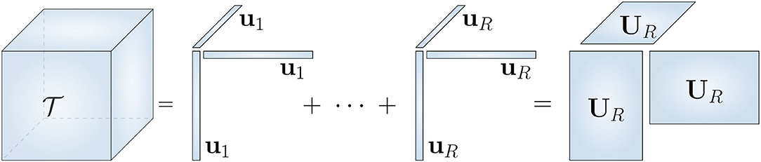
Figure 1. Polyadic decomposition of a third order symmetric tensor ${T}$. It is called canonical (CPD) if R is equal to the rank of ${T}$, i.e., R is minimal. It allows compact representation of polynomials.

3. Tensor-Based Multivariate Polynomial Optimization

The primary aim of the TeMPO framework is to develop efficient algorithms for modeling nonlinear phenomena commonly encountered in the areas of signal processing, machine learning, and artificial intelligence [15]. To achieve this, we assume structure in the nonlinear function $f:{{R}}^I\to {{R}}^N$ that maps the input data to output data. In our framework, we first assume smoothness in f and approximate it as multivariate polynomial $p:{{R}}^I\to {{R}}^N$. Then, we approximate p with low-rank tensors. This allows us to achieve efficiency both in storing the coefficients of the approximation and in performing computations with those coefficients. Although any continuous function on a compact domain can be approximated by polynomials arbitrarily well according to the Stone–Weierstrass theorem, polynomial approximations used in practice can pose several numerical issues such as the Runge phenomenon. Several strategies have been proposed to overcome these numerical issues, such as using different polynomial bases and Tikhonov regularization [38, 39]. In this work, we will focus more on computational issues of the TeMPO framework; however, it is possible to incorporate these strategies with TeMPO using slight modifications. In the remaining part of this section, we describe the scope of TeMPO. Then we will describe two types of tensor representations of multivariate polynomials where the symmetric CPD structure is imposed on the coefficient tensors. Next we will briefly describe the Gauss–Newton algorithm using the dogleg trust-region method and show how to exploit the symmetric CPD structure in the computation of Jacobian and Jacobian-vector products that are necessary for the Gauss–Newton algorithm.

3.1. Scope of the TeMPO Framework

The TeMPO framework concerns optimization problems with continuous cost functions on compact domains, namely multilinear/polynomial cost functions with or without additional constraints, which is a more general setting than tensor decomposition or retrieval of a tensor factorization. To better describe the scope, let us consider the following class of objective functions:

$\begin{array}{ll}l(\theta ,p(z)),& (5)\end{array}$

where $l:{R}\times {{R}}^M\to {{R}}^{+}$ denotes the performance measure of the model to be optimized, $p:{{R}}^I\to {R}$ denotes a multivariate polynomial represented by low-rank tensors, $z\in {{R}}^I$ denotes input data, and $\theta \in {{R}}^M$ denotes output data. A broad range of objective functions are in the class of (5). For example, the objective function for the estimation of the CPD of a third-order tensor ${T}$ can be written as

$\begin{array}{l}\frac{1}{2}\left|\right|\theta -p(A,B,C)|{|}_2^2,\text{where }p(A,B,C)=\text{vec}([A,B,C]).\end{array}$

Other tensor decomposition problems, such as block term decomposition (BTD), also fit into TeMPO. The symmetric best rank-1 approximation problem [40], which can also be formulated as

$\begin{array}{ll}{\displaystyle \underset{z\in {{R}}^I}{max}}{T}{z}^d,\text{subject to}\left|\right|z\left|\right|=1,& (6)\end{array}$

is another example problem that fits into the framework. Note that (6) is expressed as the maximization of an objective function, rather than as the decomposition of a tensor; indeed TeMPO allows one to address more general problems. For the symmetric best rank-1 approximation problem, several approaches such as higher-order power method [40], generalized Rayleigh–Newton iteration and the alternating least squares methods [41], SVD-based algorithms [42], semi-definite relaxations [43] have been proposed. Problems from unsupervised learning such as nonlinear dimensionality reduction, manifold learning, nonlinear blind source separation, and nonlinear independent component analysis also fit into TeMPO. Similarly, problems from supervised learning fit into TeMPO as well. In this work, we will focus on the regression and classification problem and derive expressions for Jacobian and Jacobian-vector products, which are necessary for the Gauss–Newton algorithm. However, the derivations here can be extended to the other problems without much effort.

Given data points $(y_k,z_k)$, the regression problem can be formulated within the TeMPO framework for the type I model as

$\begin{array}{l}{\displaystyle \underset{{{T}}_0,\dots ,{{T}}_d}{min}}p({{T}}_0,\dots ,{{T}}_d,Z)\\ ={\displaystyle \underset{{{T}}_0,\dots ,{{T}}_d}{min}}\frac{1}{2}{\displaystyle \sum _{k=1}^K}{\left(y_k-{{T}}_0-{\displaystyle \sum _{j=1}^d}{{T}}_j{z}_k^j\right)}^2,\\ \text{subject to}\text{rank}({{T}}_j)=R_j& (7)\end{array}$

where $R_j\in {\mathbb{N}}^{+}$ is a small integer, ${{T}}_j\in {{R}}^{I\times I\times \dots \times I}$ denotes the low-rank structured coefficient tensor of order j to be optimized, ${{T}}_0\in {R}$ denotes a scalar, $\text{Z}\in {{R}}^{I\times K}$ denotes the data matrix, $z_k$ denotes the kth column of Z and K is the number of available data points. For the type II model, the regression problem takes the form

$\begin{array}{l}{\displaystyle \underset{{T}}{min}}p({T},\tilde{z})={\displaystyle \underset{{T}}{min}}\frac{1}{2}{\displaystyle \sum _{k=1}^K}{\left(y_k-{T}{\tilde{z}}_i^d\right)}^2,\\ \text{subject to}\text{rank}({T})=R& (8)\end{array}$

where ${T}$ denotes the low-rank structured coefficient tensor of order d to be optimized, $\tilde{\text{Z}}\in {{R}}^{(I+1)\times K}$ denotes the augmented input data matrix, and $\widetilde{z_k}$ denotes the kth column of $\tilde{\text{z}}$, i.e., ${\tilde{z}}_k=\left[1;z_k\right]$.

3.2. Tensor Representation of Polynomials

In this subsection, we examine the type I and type II model in detail. A (symmetric) tensor ${T}$ of order d and dimension n can be associated with a homogeneous n-variate polynomial $p(z)$ of degree d [44], as shown in Equation (3).

Type I: Since any polynomial can be written as a sum of homogeneous polynomials of increasing degrees, any polynomial of degree d can be written by using tensors of order up to d, as shown in Equation (2). Note that in the tensor representation of polynomials, any tensor can be assumed to be symmetric without loss of generality. Indeed, any homogeneous polynomial $p(z)$ of degree d ∈ ℕ can be represented by a multilinear form ${T}{z}^d$, where ${T}\in {𝕂}^{I\times I\times \dots \times I}$ is a symmetric tensor of order d and $z\in {𝕂}^I$.

To see this, suppose a homogeneous polynomial $p(z)$ is represented as

$\begin{array}{l}p(z)=\tilde{{T}}{z}^d={\displaystyle \sum _{i_1,i_2.\dots ,i_d=1}^I}{\tilde{t}}_{i_1{i}_2\dots i_d}{z}_{i_1}{z}_{i_2}\dots z_{i_d},\end{array}$

where $\tilde{{T}}\in {𝕂}^{I\times I\times \dots \times I}$ is a tensor of order d. Since the terms z_i1z_i2…z_id are invariant under the permutation of indices, we may write

$\begin{array}{l}\hfill p(x)={\displaystyle \sum _{i_1,i_2.\dots ,i_d=1}^I}{t}_{i_1{i}_2\dots i_d}{z}_{i_1}{z}_{i_2}\dots z_{i_d},\hfill \\ \hfill \text{where}{t}_{i_1{i}_2\dots i_d}=\frac{1}{d!}{\displaystyle \sum _{(i_1,i_2,\dots ,i_d)\in \Pi (i_1{i}_2\dots i_d)}}{\tilde{t}}_{i_1{i}_2\dots i_d},\hfill \end{array}$

here Π(i₁i₂ … i_d) denotes the collection of all permutation of indices (i₁, i₂, …, i_d). Since the entries of ${T}$ are invariant under the permutation of indices, we can conclude that ${T}$ is symmetric.

The above discussion reveals the fact that there are infinitely many representations of a given polynomial. Indeed two representations with tensors ${T}$ and ${W}$ are equal so long as the summation of the corresponding entries over the permutation of indices remains the same, i.e.,

$\begin{array}{l}{\displaystyle \sum _{(i_1,i_2,\dots ,i_d)\in \Pi (i_1{i}_2\dots i_d)}}{t}_{i_1{i}_2\dots i_d}={\displaystyle \sum _{(i_1,i_2,\dots ,i_d)\in \Pi (i_1{i}_2\dots i_d)}}{w}_{i_1{i}_2\dots i_d}\end{array}$

In the ANOVA kernel used in higher-order factorization machines, all t_{Π(i1i2…id)} are set to zero except t_{(i1<i2 < … < id)} [31], which leads to a sparse representation. In this paper, we use symmetric tensors for two reasons. The first reason is that the CPD of a symmetric tensor can be expressed by a single factor matrix. Therefore, the symmetric CPD representation of multivariate polynomial requires fewer number of parameters in comparison with a non-symmetric representation. The second reason is that there is a rich history of the representation of polynomials with symmetric tensors in the field of algebraic geometry under the name of the Waring problem [45].

Type II: Augmenting the independent variable vector $z$, by a constant 1¹, i.e., $\tilde{z}=\left[1;z^{\mathrm{\text{T}}}\right]$ leads to a different representation of non-homogeneous polynomials that uses a single dth order symmetric tensor for the inhomogeneous multivariate polynomial of degree d, as shown in Equation (3). This process is called homogenization [46] and is graphically illustrated in Figure 2. If we just use full tensors, the type I and II models are interchangeable. However, it is important to note that when low-rank structure is imposed on the coefficient tensors, both representations yield different classes of low-rank multivariate polynomial. Hence, these approaches may lead to different results depending on the application. The former approach requires more parameters since it uses more factor matrices. The difference in the number of parameters should be taken into account to prevent underfitting and overfitting. A more detailed description for storage complexity is given in Section 3.5. Moreover, the type I model allows us to constrain each term in the representation separately. In modeling multivariate polynomials, one might not wish the terms of different order to have some shared structure, in which case one should choose the type I model to work with. Similarly, the type II model should be chosen, if some shared structure is desired in the terms of different order. To further elaborate on the effects of homogenization on the rank of a tensor, let us consider the following proposition.

FIGURE 2

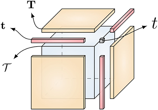
Figure 2. By applying the homogenization process, symmetric tensors can represent the coefficients of non-homogeneous polynomials. For example, by stacking the coefficients t, t, T, and ${T}$ of the third degree polynomial into a tensor as shown above, we can represent it with a symmetric third-order tensor. Image reproduced from Debals [46].

Proposition 1. Let $p(z):{{R}}^I\to {R}$ be a multivariate polynomial of order d defined as in equation (2) by a scalar ${{T}}_0$ and symmetric tensors ${{T}}_j\in {{R}}^{I\times I\times \dots \times I}$ for j = 1, 2, …, d. Moreover, let ${W}\in {{R}}^{(I+1)\times \dots \times (I+1)}$ be the corresponding tensor obtained from the homogenization process. The tensors ${W}$ and ${{T}}_j$ have the same rank R if and only if the tensors ${{T}}_j$ admit unique CPDs with shared factor matrices and a weight vector $c$, i.e.,

$\begin{array}{l}{\displaystyle {{T}}_j={\displaystyle 〚U,\dots ,U;C_d^j{(c^{\text{T}})}^{\odot (d-j)}〛},\text{and}{{T}}_0={\displaystyle \sum _{r=1}^R}{\left({(c^{\text{T}})}^{\odot d}\right)}_r.}\end{array}$

Proof 1. Let the CPD of the tensor ${W}$ be defined as 〚V, …, V〛, where, for convenience but without loss of generality, the weights of the rank-1 terms are assumed to be 1. Since ${W}$ is obtained by the homogenization process, partitioning V as $\left[v^{\mathrm{\text{T}}};\text{Q}\right]$ and using the definition of CPD, we obtain

$\begin{array}{ll}{{T}}_j=〚Q,\dots ,Q;C_d^j{(v^{\text{T}})}^{\odot (d-j)}〛,\text{and}{{T}}_0={\displaystyle \sum _{r=1}^R}{\left({(v^{\text{T}})}^{\odot d}\right)}_r.& (9)\end{array}$

Since the CPDs of the tensors ${{T}}_j$ are unique, the equality (9) holds if and only if the equalities Q = U and $v=c$ also hold.

Remark 1. In the above proof, we assumed that the vector $v$ does not contain any zero elements. Note that if the vector $v$ does contain zero elements, it cancels the corresponding rank-1 terms. Therefore, in that case $\mathrm{\text{rank}}({W})>\mathrm{\text{rank}}({{T}}_j)$, for j = 1, …, d−1. Moreover, the uniqueness of the CPDs of ${{T}}_j$ implies that $\mathrm{\text{rank}}({W})\ge \mathrm{\text{rank}}({{T}}_j)$. Since the equality $\mathrm{\text{rank}}({W})=\mathrm{\text{rank}}({{T}}_j)$ holds only when the tensors ${{T}}_j$ have shared factor matrices as described above, we can conclude that in all other cases $\mathrm{\text{rank}}({W})>\mathrm{\text{rank}}({{T}}_j)$.

Proposition 1 together with Remark 1 reveals the fact that if ${W}$ admits a rank-R CPD, there exists tensors ${{T}}_j$ that admit rank-R_j CPDs with shared factors and R_j ≤ R. Hence, the expressive power of the type II model is weaker than the type I model, i.e., the type II model requires higher rank values than the type I model to be able to model functions of the same complexity. In other words, the set of polynomials represented by the type II model is a strict subset of the set of polynomials represented by the type I model for the same rank values.

Although we focus in this study on the type I and type II models in the symmetric CPD format, the TeMPO framework is not limited to these. TeMPO collects low-rank tensor representations of multivariate polynomials under a roof by utilizing various other tensor decompositions such as TT, HT, and non-symmetric and partially symmetric CPD formats². In this way, TeMPO breaks the curse of dimensionality and makes it possible to develop second-order efficient algorithms for the optimization of a more general class of multivariate polynomials. Moreover, use of structured tensors and multilinear algebra makes it easy to incorporate other polynomial bases and, more generally, other nonlinear feature maps rather than the standard polynomial bases to the TeMPO framework. From this point of view, TeMPO can be interpreted as a generalization of higher-order factorization machines that use particular types of multivariate polynomials with the standard polynomial bases and utilize first-order and BFGS type algorithms [30–32, 47].

3.3. Gauss–Newton Algorithm

Most standard first-order and second-order numerical optimization algorithms can be used for solving problem (8). Since the objective function under consideration is a least-squares function, we will utilize the second-order batch Gauss–Newton (GN) algorithm using a trust-region to take advantage of its attractive properties such as quadratic convergence near a local optimum point, resistant to swamps, suitable to incorporate constraints easily and eligible to exploit multilinear structure. In the case the objective function is not least squares, the inexact GN algorithm can also be utilized. Below, we briefly describe the GN algorithm using a trust-region, and then derive the expressions for Jacobian and Jacobian-vector products for tensors in the symmetric CPD format. In nonlinear least-squares problems, the objective function is the squared error between a data vector $y$ and a nonlinear model $m(z)$ [6, 33]:

$\begin{array}{ll}f(z)=\frac{1}{2}\left|\right|m(z)-y|{|}_2^2=\frac{1}{2}{r}^{\text{T}}r,& (10)\end{array}$

where $z\in {{R}}^I$. The algorithm updates the initial guess iteratively by taking a step length α_k in the direction $p_k$ at the iteration k, i.e.,

$\begin{array}{l}{z}_k=z_{k-1}+{\alpha }_k{p}_k,\end{array}$

until some stopping criteria are satisfied. Line search and trust-region are the two main approaches used to determine α_k and $p_k$. Here, we focus on the dogleg trust-region approach. In this approach, one sets α_k = 1. Then, given a trust-region of radius δ_k, the GN step $p_k^{gn}$ and the steepest descent step $p_k^{sd}$ for the current iteration, the step direction $p_k$ is determined by the following procedure:

• If $\left|\right|p_k^{gn}|{|}_2\le {\delta }_k$, then $p_k=p_k^{gn}$.

• If $\left|\right|p_k^{gn}|{|}_2>{\delta }_k$ and $\left|\right|p_k^{sd}|{|}_2>{\delta }_k$, then $p_k={\delta }_k{p}_k^{sd}/\left|\right|p_k^{sd}|{|}_2$.

• If $\left|\right|p_k^{gn}|{|}_2>{\delta }_k$ and $\left|\right|p_k^{sd}|{|}_2\le {\delta }_k$, then $p_k={\tau }_k{p}_k^{sd}+{\beta }_k(p_k^{gn}-{\tau }_k{p}_k^{sd})$, where ${\tau }_k=-\left|\right|p_k^{sd}|{|}_2^2/|\left|{\text{J}}_k{p}_k^{sd}\right|{|}_2^2$, and β_k is selected such that $\left|\right|p_k|{|}_2={\delta }_k$.

The steepest descent step $p_k^{sd}$ is given by $-{\text{J}}_k^{\mathrm{\text{T}}}{r}_k$. To compute the GN step, a second order Taylor series approximation for the objective function is used. The optimal direction for the GN step $p_k^{gn}$ can be obtained by solving the optimization problem,

$\begin{array}{ll}{p}_k^{gn}={\displaystyle \underset{p}{argmin}}\tilde{f}(p),\text{with}\tilde{f}(p)=f(z_k)+p^{\text{T}}{g}_k+\frac{1}{2}{p}^{\text{T}}{H}_{k}p,& (11)\end{array}$

where $g_k$ denotes the gradient and H_k denotes the Hessian at the current iteration. Setting $\partial \tilde{f}(p)/\partial p$ to zero, the solution of (11) can be obtained by solving the linear system of equations

$\begin{array}{ll}{H}_k{p}_k^{gn}=-g_k,\text{with}{g}_k=J_k^{\text{T}}{r}_k,& (12)\end{array}$

where J_k denotes the Jacobian of $f(z_k)$ at iteration k, and $r_k=m(z_k)-y$. However, in real-life applications, explicit computation of the Hessian is often expensive. To overcome this, GN approximates the Hessian by the Grammian matrix as

$\begin{array}{l}{H}_k\approx J_k^{\text{T}}{J}_k.\end{array}$

In this study, we used the conjugate gradient (CG) algorithm for solving (12) together with the dogleg trust-region approach which is implemented in Tensorlab [11]. The overall algorithm is summarized in Table Algorithm 1.

ALGORITHM 1

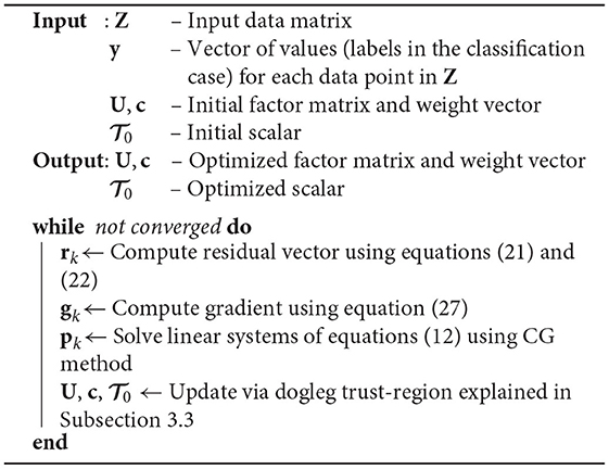
Algorithm 1. GN algorithm using dogleg trust-region for the type II model.

3.4. Exploiting the Symmetric CPD Format

As described above, the GN algorithm minimizes a cost function in the form of Equation (10). The gradient of this objective function can be written as ${\text{J}}^{\mathrm{\text{T}}}r$, and the Hessian is approximated by J^TJ, where J is the Jacobian matrix composed of partial derivatives of the residual vector $r$. Hence, it is sufficient to derive expressions for the Jacobian and Jacobian-vector products. We begin with the first-order derivatives of the multilinear form ${T}{z}^d$, where ${T}$ is in the symmetric CPD format, with respect to its factors and then proceed to the derivation of Jacobian and Jacobian-vector products for problems (7) and (8). The derivations made here can be used in other TeMPO problems with slight modifications.

3.4.1. Derivatives of the Multilinear Form in the Symmetric CPD Format

By using the matrix unfolding of the tensor in the symmetric CPD format and Property 2 of Khatri–Rao product, the multilinear form ${T}{z}^d$ can be written as

$\begin{array}{ll}{T}{z}^d=c^{\text{T}}{\left(U^{\text{T}}z\right)}^{*d},& (13)\end{array}$

which will be useful for our derivations below.

Lemma 1. Let ${T}\in {𝕂}^{I\times I\times \dots \times I}$ be a symmetric tensor of order d and its CPD given as ${T}=〚\text{U},\dots ,\text{U};c^{\mathrm{\text{T}}}〛$. Then the derivative of the multilinear form ${T}{z}^d$ with respect to vec(U) can be obtained as

$\begin{array}{l}\frac{\partial {T}{z}^d}{\partial \text{vec}(U)}={\left((c*w)\otimes z\right)}^{\text{T}},\end{array}$

where $w=d{({\text{U}}^{\mathrm{\text{T}}}z)}^{*\left(d-1\right)}$.

Proof 2. The proof immediately follows from Equation (13) and successive application of Property 3.

Lemma 2. Let ${T}\in {𝕂}^{I\times I\times \dots \times I}$ be symmetric tensor of order d and its CPD is given as ${T}=〚\text{U},\dots ,\text{U};c^{\mathrm{\text{T}}}〛$. Then the derivative of multilinear form ${T}{z}^d$ with respect to vector $c$ can be obtained as

$\begin{array}{l}\frac{\partial {T}{z}^d}{\partial c}={(z^{\text{T}}U)}^{*d}.\end{array}$

Proof 3. The proof immediately follows from Property 3 and Equation (13).

3.4.2. Exploiting Structure in the Type I Model

Objective Function: The construction of the residual vector $r$ and the computation of its l₂ norm is sufficient for computing the objective function in (7). By utilizing Property 2 and Equation (13), the residual vector can be expressed as $r=y-\mu$, where each entry of the vector $\mu \in {{R}}^K$ is defined as

$\begin{array}{l}{\mu }_k={{T}}_0+{\displaystyle \sum _{j=1}^d}{c}_j^{\text{T}}{w}_{j,k}^{*j},\end{array}$

in which $w_{j,k}={\text{U}}_j^{\mathrm{\text{T}}}{z}_k$ with ${\text{U}}_j\in {{R}}^{I\times R}$, and $w_{j,k}^{*j}$ denotes the jth elementwise power of the vector $w_{j,k}$. By defining ${\text{W}}_j=\left[w_{j,1},w_{j,2},\dots ,w_{j,K}\right]$, we can write the residual vector $r$ in a compact form as

$\begin{array}{ll}r=y-{{T}}_0·1_K-{\displaystyle \sum _{j=1}^d}{(c_j^{\text{T}}\left(W_j^{*j}\right))}^{\text{T}},& (14)\end{array}$

Using the above Equation (14), the objective function can be computed as the l₂ norm of the residual vector $r$.

Jacobian: The Jacobian matrix for problem (7), with the tensors ${{T}}_j$ in their symmetric CPD format, can be written in a compact form as

$\begin{array}{l}J=\left[J_1;\dots ;J_K\right],\text{where}\\ J_k=\left[1,\frac{\partial r_k}{\partial \text{vec}(U_1)},\dots ,\frac{\partial r_k}{\partial \text{vec}(U_d)},\frac{\partial r_k}{\partial c_1},\dots ,\frac{\partial r_k}{\partial c_d}\right].& (15)\end{array}$

Note that we used the fact $\partial r_k/\partial {{T}}_0=1$ in the above equation. By utilizing Lemma 1 and Lemma 2, the derivative of each term of the residual vector with respect to U_j and $c_j$ can be expressed as

$\begin{array}{ll}\frac{\partial r_k}{\partial \text{vec}(U_j)}=-j{\left[\left(c_j*w_{j,k}^{*\left(j-1\right)}\right)\otimes z_k\right]}^{\text{T}},\text{and}\frac{\partial r_k}{\partial c_j}={\left(w_{j,k}^{*j}\right)}^{\text{T}}.& (16)\end{array}$

By defining ${\tilde{\text{W}}}_j=-j\left({\text{W}}_j^{*\left(j-1\right)}\right)$ for j = 1, …, d, and $\text{Z}=\left[z_1,z_2,\dots ,z_K\right]$, the Jacobian matrix J in (15) can be obtained in the following compact block form:

$\begin{array}{ll}J=\left[1_K,{((C_1{\tilde{W}}_1)\odot Z)}^{\text{T}},\dots ,{((C_d{\tilde{W}}_d)\odot Z)}^{\text{T}},V\right],& (17)\end{array}$

where V is a K × d block matrix in which each block is defined as ${\text{V}}_{k,j}={\left(w_{j,k}^{*j}\right)}^{\mathrm{\text{T}}}$, ${\text{C}}_j=\mathrm{\text{Diag}}(c_j)$, and d is the degree of the polynomial under consideration. Since we only need the Jacobian-vector products for the GN algorithm, the explicit construction of the Jacobian matrix is not required. The Jacobian-vector products can be obtained in a more memory-efficient way as described below.

Jacobian-Vector Product: The product of Jacobian J by a vector $x$ can be obtained using block matrix operations. The product of each block term by a vector $\mathrm{\text{vec}}({\text{X}}_j)=x_j$ can be obtained by utilizing properties 1 and 2 as

$\begin{array}{ll}{((C_j{\tilde{W}}_j)\odot Z)}^{\text{T}}{x}_j={\left[\left(X{\text{T}}_{j}Z\right)*\left(C_j{\tilde{W}}_j\right)\right]}^{\text{T}}{1}_R.& (18)\end{array}$

Note that the multiplication of a matrix by 1_R from the right is equivalent to summing the columns of the matrix under consideration. Therefore, neither the multiplication by 1_R nor the transposition of the matrix $\left({\text{X}}_j^{\mathrm{\text{T}}}\text{Z}\right)*\left({\text{C}}_j{\tilde{\text{W}}}_j\right)$ in Equation (18) is necessary to obtain the Jacobian-vector product. Note also that, since the matrices C_j are diagonal, the product ${\text{C}}_j{\tilde{\text{W}}}_j$ can be obtained in a memory efficient way by multiplying the rows of ${\tilde{\text{W}}}_j$ by the corresponding diagonal elements of C_j without explicitly forming the matrices C_j. Overall, the product of the Jacobian J and the vector $x$ can be obtained by partitioning the vector $x$, i.e., $x=\left[x_1;x_1;x_2;\dots ;x_d;x_v\right]$, and by using the Equations (17) and (18) as

$\begin{array}{l}Jx=x_1·1_K+{\displaystyle \sum _{j=1}^d}{\left[\left(X_j^{\text{T}}Z\right)*\left(C_j{\tilde{W}}_j\right)\right]}^{\text{T}}{1}_R+V{x}_v,\end{array}$

where ${\text{X}}_j=\mathrm{\text{unvec}}(x_j)$.

Jacobian Transpose -Vector Product and Gradient: In a similar way, block-wise multiplication of the Jacobian transpose J^T by a vector can be obtained from the expression

$\begin{array}{ll}((C_j{\tilde{W}}_j)\odot Z)x=\text{vec}\left(Z\text{Diag}(x){(C_j{\tilde{W}}_j)}^{\text{T}}\right).& (19)\end{array}$

Note that right multiplication by a diagonal matrix can be done efficiently by only multiplying the columns of the matrix with the corresponding diagonal elements without explicitly forming the diagonal matrix. Overall, by defining ${\xi }_j=\mathrm{\text{vec}}\left(\text{Z}\mathrm{\text{Diag}}(x){({\text{C}}_j{\tilde{\text{W}}}_j)}^{\mathrm{\text{T}}}\right)$, we can obtain the product of the Jacobian transpose J^T and a vector x in the following form:

$\begin{array}{ll}{J}^{\text{T}}x=\left[{\displaystyle \sum _{k=1}^K}{x}_k;{\xi }_1;{\xi }_2;\dots ;{\xi }_d;V^{\text{T}}x\right].& (20)\end{array}$

The gradient can be obtained by the product of the Jacobian transpose J^T and the residual vector $r$. Defining ${\eta }_j=\mathrm{\text{vec}}\left(\text{Z}\mathrm{\text{Diag}}(r){({\text{C}}_j{\tilde{\text{W}}}_j)}^{\mathrm{\text{T}}}\right)$ and utilizing the Equations (19) and (20), we can obtain the gradient as

$\begin{array}{l}g=\left[{\displaystyle \sum _{k=1}^K}{r}_k;{\eta }_1;{\eta }_2;\dots ;{\eta }_d;V^{\text{T}}r\right].\end{array}$

3.4.3. Exploiting Structure in the Type II Model

Objective Function: The computation of the objective function for the type II model is similar to that of the type I model. Utilizing Property 2 and Equation (13), the residual vector for problem (8) can be obtained as $r=y-\mu$ with

$\begin{array}{ll}\mu =\left[c^{\text{T}}{w}_1^{*d};c^{\text{T}}{w}_2^{*d};\dots ;c^{\text{T}}{w}_K^{*d}\right],& (21)\end{array}$

where $w_k={\text{U}}^{\mathrm{\text{T}}}{\tilde{z}}_k$. By defining $\text{W}=\left[w_1,w_2,\dots ,w_K\right]$, we can write the residual vector $r$ in a compact form as

$\begin{array}{ll}r=y-{\left(c^{\text{T}}\left(W^{*d}\right)\right)}^{\text{T}},& (22)\end{array}$

Using the above Equation (22), the objective function can be computed as the l₂ norm of the residual vector $r$.

Jacobian: The Jacobian matrix of the cost function in (8) can be defined in a compact form as

$\begin{array}{ll}J=\left[J_1;J_2;\dots ;J_K\right],\text{where}{J}_k=\left[\frac{\partial r_k}{\partial \text{vec}(U)},\frac{\partial r_k}{\partial c}\right].& (23)\end{array}$

Utilizing Lemma 1 and Lemma 2 and using the equations in (16), the parts of J_k in Equation (23) can be written as

$\begin{array}{l}\frac{\partial r_k}{\partial \text{vec}\left(U\right)}=-d{\left[\left(c*w_k^{*\left(d-1\right)}\right)\otimes {\tilde{z}}_k\right]}^{\text{T}},\frac{\partial r_k}{\partial c}={\left(w_k^{*d}\right)}^{\text{T}}.\end{array}$

By defining $\tilde{\text{W}}=-d\left({\text{W}}^{*(d-1)}\right)$, $\text{V}=\left[\frac{\partial r_1}{\partial c};\frac{\partial r_2}{\partial c};\dots ;\frac{\partial r_K}{\partial c}\right]$, and $\text{Z}=\left[{\tilde{z}}_1,{\tilde{z}}_2,\dots ,{\tilde{z}}_K\right]$, the Jacobian matrix can be obtained in the following compact form:

$\begin{array}{ll}J=\left[{\left((C\tilde{W})\odot Z\right)}^{\text{T}},V\right].& (24)\end{array}$

As mentioned earlier, explicit construction of the Jacobian matrix J is not required. We only require the Jacobian-vector and Jacobian transpose-vector products and derive efficient expressions for these products below.

Jacobian-Vector Product: The product of the Jacobian matrix J and a vector $x$ can be obtained in a similar way as for the type I model, by partitioning the vector $x$, i.e., $x=\left[x_u;x_c\right]$ and utilizing properties 1 and 2 and Equation (24), as

$\begin{array}{ll}Jx={\left[\left(X{\text{T}}_{u}Z\right)*\left(C\tilde{W}\right)\right]}^{\text{T}}{1}_R+V{x}_c,& (25)\end{array}$

where ${\text{X}}_u=\mathrm{\text{unvec}}(x_u)$. As mentioned earlier for Equation (18), explicit construction of the diagonal matrix C is not required. The product $\text{C}\tilde{\text{W}}$ can be obtained in a memory efficient way by multiplying the rows of $\tilde{\text{W}}$ by the corresponding diagonal elements of C.

Jacobian Transpose -Vector Product and Gradient: In similar way, utilizing properties 1 and 2 and Equation (24), the product of Jacobian transpose J^T and a vector $x$ can be written as

$\begin{array}{ll}{J}^{\text{T}}x=\left[\text{vec}\left(Z\text{Diag}(x){(C\tilde{W})}^{\text{T}}\right);V^{\text{T}}x\right].& (26)\end{array}$

Since the gradient is the product of the Jacobian transpose J^T and the residual vector $r$, it directly follows from the above Equation (26) as

$\begin{array}{ll}g=\left[\text{vec}\left(Z\text{Diag}(r){(C\tilde{W})}^{\text{T}}\right);V^{\text{T}}r\right].& (27)\end{array}$

3.5. Complexity Analysis

We now analyze the storage and computational complexity of TeMPO where we are optimizing over symmetric rank-R CPD structured tensors ${T}\in {𝕂}^{I\times I\times \dots \times I}$ of order d. The analysis is presented here for the type II model. However, since the number of optimization parameters of the type I and type II models (see Equations 2, 3) for an I-variate polynomial of degree d are proportional to each other, the analysis also applies to the type I model. Indeed, the computational complexity of the type I model is d times the computational complexity of the type II model. We also compare with the storage and computational complexity of TT and PEPS tensor networks.

Representing a multivariate polynomial with I independent variables and of degree d in dense format requires storing $C_{(I+d)}^d$ elements. Using Stirling's approximation, it can be shown that the storage complexity for a multivariate polynomial represented in dense format is ${O}\left(I^d\right)$ for d ≪ I. In the symmetric CPD format, we need to store only the factor matrix $\text{U}\in {{R}}^{I\times R}$ and the vector of weights $c\in {{R}}^R$, where R is the rank of the symmetric CPD. Therefore, the storage complexity for the type II model using the symmetric CPD format is ${O}(IR)$. This shows that the symmetric CPD format breaks the curse of dimensionality, since the storage complexity in this format is linear in terms of rank R and dimension I.

As is clear from Equation (22), the construction of the matrix W and its dth Hadamard (elementwise) power dominates the computational complexity of the objective function. The construction of a single column of the matrix W requires the multiplication of ${\text{U}}^{\mathrm{\text{T}}}\in {{R}}^{R\times I}$ and ${\tilde{z}}_k\in {{R}}^I$. Thus, the computational complexity of constructing the matrix W is ${O}(IKR)$. The dth Hadamard power of the matrix W can be computed recursively by using the relation W^*(2m) = (W^*m)^*2. Thus, the computational complexity of the dth Hadamard power of the matrix $\text{W}\in {{R}}^{R\times K}$ is ${O}(log(d)RK)$. Therefore, the total computational complexity for computing the objective function for a batch of size K is ${O}((I+log(d))KR)$. Since log(d) ≪ I, the computational complexity for the objective function in Equation (8) is ${O}(IKR)$.

The gradient of the objective function in Equation (8) can be obtained by multiplying the Jacobian transpose J^T by the residual vector $r$. As shown in Equation (27), this operation requires multiplication of a matrix $\text{Z}\in {{R}}^{I\times K}$ by a diagonal matrix $\mathrm{\text{Diag}}(r)$, and the multiplication of the matrices $\text{Z}\mathrm{\text{Diag}}(r)$ and ${(\text{C}\tilde{\text{W}})}^{\mathrm{\text{T}}}$ with sizes (I × K) and (K × R), respectively. Note that the entries of the product $\text{C}\tilde{\text{W}}$ were already obtained in the computation of the objective function. Further, the computational complexity for the product $\text{Z}\mathrm{\text{Diag}}(r)$ is ${O}(IK)$. Consequently, the computational complexity for the multiplication of $\text{Z}\mathrm{\text{Diag}}(r)$ and ${(\text{C}\tilde{\text{W}})}^{\mathrm{\text{T}}}$ is ${O}(IKR)$. In addition, the computation of ${\text{V}}^{\mathrm{\text{T}}}r$ in Equation (27) requires ${O}(KR)$ operations. However KR ≪ IKR. Therefore, the total computational complexity for computing the gradient is ${O}(IKR)$ for R ≫ 1.

In addition, TeMPO uses the GN algorithm for the optimization. However, this is not a requirement and first-order methods can also be utilized within TeMPO as well. GN requires solving the linear system of equations in (12). Tensorlab's implementation of GN uses the conjugate-gradient (CG) method which requires only the Grammian-vector product for solving (12). This operation requires multiplication of the Jacobian and its transpose by a vector. The computational complexity of multiplying the transpose of Jacobian by a vector is ${O}(IKR)$ as described above. The computationally most expensive operations in the multiplication of Jacobian by a vector are the multiplication of matrices ${\text{X}}_u^{\mathrm{\text{T}}}$ and Z with sizes (R × I) and (I × K), and the Hadamard product of two matrices of size (R × K) as shown in Equation (25). Hence, the computational complexity of computing $\text{J}x$ is ${O}(IKR)$. Note that the entries of the product $\text{C}\tilde{\text{W}}$ were already obtained in the computation of the objective function. Therefore, the total computational complexity for a single CG iteration is ${O}(2IKR)$. Note that a large number of CG iterations in the solution of linear equations for the GN algorithm might increase the computation time compared to first-order algorithms. In fact, the number of CG iterations scales with the number of optimization variables (IR), if the exact solution is desired in the solution of the normal equations. This may lead to an quadratic complexity of ${O}(2{(IR)}^{2}K)$. However, we observed in our experiments that a small number of CG iterations were sufficient to obtain accurate results. For example, we set the maximum number CG iterations to 10 for the classification of the MNIST and Fashion MNIST datasets, where the number of unknowns is 784 × R with R ranging from 10 to 150.

The storage complexity of a tensor network with TT architecture is bounded by ${O}(nI{R}_{TT}^2)$ for a tensor of order I with dimensions (n × n × … × n), where R_TT denotes the TT-rank [48]. n is equal to 2 and I is the size of a single image in the image classification applications presented in [20, 21]. Note that the storage complexity of TT increases with powers of the TT-rank R_TT. The total computational complexity of TT for computing the objective function has been reported as ${O}(nI{R}_{TT}^2+R_{TT}^{3}log(I))$, when the contraction order defined in [21] is used. When the sweeping algorithm described in [20] is used, the computational complexity of the objective function for TT is ${O}(n^3{R}_{TT}^{3}I)$ for a single data point of size I. Similar to the storage complexity, the computational complexity of the objective function for TT increases with powers of the TT-rank of the tensor under consideration. On the other hand, automatic differentiation (AD) is one of methods used to compute the gradient of TT. The computational complexity of automatic differentiation is linear in the complexity of the evaluation of the objective function [49]. Therefore, the computational complexity of the gradient for TT tensor network presented in [21] is ${O}(\alpha (nIK{R}_{TT}^2+K{R}_{TT}^{3}log(I)))$, for a batch size of K with α > 1. The total computational complexity of TT tensor network for a batch size of K has been reported as ${O}(m{R}_{TT}^2(R_{TT}+K))$ for a single iteration of the stochastic Riemannian gradient descent algorithm [19]. As it is clear from the above discussion, both the storage and the computational complexity of TT increases with a power of the TT-rank regardless of the algorithm used, while for TeMPO it increases linearly with the symmetric CPD rank in the symmetric CPD case.

The computational complexity of a single forward pass of PEPS for a batch size of K is ${O}(K{R}_{BT}^3{R}_{PS}^6)$, when the boundary matrix product state method is used. Here R_BT is the bond dimension (rank) of the boundary matrix product state of PEPS and R_PS is the bond dimension of PEPS. In addition, the backward pass for PEPS requires ${O}(\alpha K{R}_{BT}^3{R}_{PS}^6)$ operations (with α > 1), when automatic differentiation is used [22].

The above analysis shows that TeMPO is computationally less expensive than TT and PEPS, even though it uses a second-order algorithm. All these results are summarized in Table 1. The fundamental reason for this is the linear storage complexity of the symmetric CPD format. Both TT and PEPS involve third and higher-order tensors, which makes their computational complexity increase with powers of the bond dimension. On the other hand, the CPD format is known to be numerically less stable than the TT format, which relies on orthogonal matrices.

TABLE 1

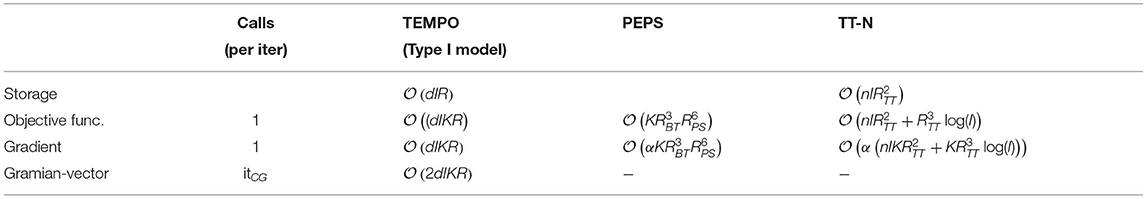
Table 1. The comparison of the computational complexity of TEMPO with TT and PEPS tensor networks for a batch size of K.

4. Numerical Experiments

We conducted an experiment on the regression problem using synthetic data to illustrate the TeMPO framework and compared TeMPO with different implementations of SVMs in Section 4.1. Next, we applied our framework to the blind deconvolution of constant modulus (CM) signals and compared with the analytical CM algorithm (ACMA) [50], the optimal step-size CM algorithm (OSCMA) [51], and the LS-CPD framework [52] in Section 4.2. In Section 4.3, we further illustrate TeMPO with the image classification problem. We performed experiments on the MNIST and Fashion MNIST datasets and compared the accuracy and number of optimization parameters with MLPs, and TT and PEPS tensor networks. We performed experiments on a computer with an Intel Core i7-8850H CPU at 2.60 GHz with 6 cores and 32 GB of RAM using MATLAB R2021b and Tensorlab 3.0 [11].

In our blind deconvolution experiments, we used the complex GN algorithm with the conjugate gradient Steihaug method. We used the second-order batch Gauss–Newton algorithm for the regression and classification, following the same intuition as in [53]. In each epoch of the algorithm, we randomly shuffle the data points in the training set and process all data points by dividing them into batches. In the regression and binary classification case, we optimize a single cost function. In the multi-label classification case, for each batch, we randomly select a cost function f_l defined for each label to optimize. Thus our algorithm does not guarantee that each f_l will be trained by all training images in each epoch in the multi-label classification case. To guarantee this, the algorithm can be modified such that for each batch all cost functions f_l are optimized at the cost of increasing CPU time by a factor of the number of classes L. However, in that case the algorithm might need fewer epochs to converge. The overall algorithm is summarized in Algorithm 2. Algorithm 2 is given for the type II model for the ease of explanation. Slight modifications are sufficient to obtain an algorithm for the type I model.

ALGORITHM 2

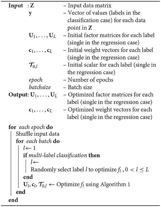
Algorithm 2. Batched GN algorithm using dogleg trust-region for regression and classification for the type II model.

We define the relative error as the relative difference in l₂ norm $\left|\right|f-\hat{f}|{|}_2/|\left|f\right|{|}_2$ with $\hat{f}$ an estimate for a vector $f$, and the signal-to-noise ratio (SNR) as $20{log}_{10}(||f|{|}_2/||\eta |{|}_2)$, where $\eta =\hat{f}-f$.

4.1. Regression

In this experiment, we considered a low-rank smooth function $f(x):{{R}}^N\to {R}$, namely

$\begin{array}{ll}f(x)={\displaystyle \sum _{r=1}^{R_f}}{\alpha }_r{e}^{(a_r^{\text{T}}x)},& (28)\end{array}$

where $x\in {\left[-1,1\right]}^N$, R_f is the rank of the function $f(x)$, and the coefficients α_r are scalars randomly chosen from the standard normal distribution. We generated 5, 000 test samples and 1, 000 training samples for N = 50 and R_f = 8. Each vector $a_r\in {{R}}^N$ was a unit norm vector drawn from the standard normal distribution. Each of the samples of $x$ was drawn from the uniform distribution. We initialized each factor matrix with a matrix whose elements were randomly drawn from the standard normal distribution, and scaled it to unit norm. We initialized each weight vector in the same way as the factor matrices. We approximated $f(x)$ by the type I and type II model of degree 5 whose coefficient tensors were represented in the rank-R symmetric CPD format. We set the batch size to 500 and the maximum number GN iterations to 5 for each batch. In Figure 3, we show the median relative test and training errors for R = {2, 4, 8, 16} as a function of the number of epochs for 100 trials. Each epoch corresponds to optimization over the full training set. It is clear from Figure 3 that TeMPO produces more accurate results and generalizes better when using higher rank values, for both the type I and type II model. Good performance is also observed for R = 16 > R_f = 8, meaning that TeMPO is robust to over-estimation of the number of parameters. For low rank values, i.e., R < R_f, the type I model produces better results than the type II model because it involves more parameters that can be tuned, cf. the discussion of Proposition 1.

FIGURE 3

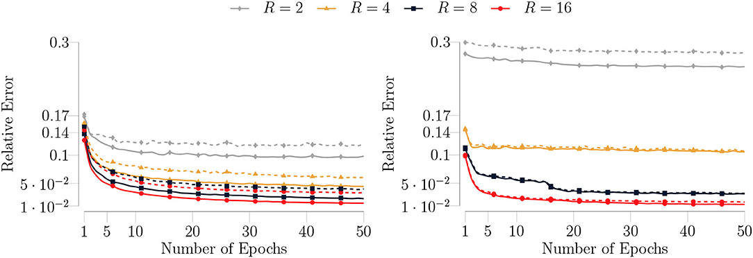
Figure 3. (Left) The median test (dashed lines) and training (solid lines) errors of the type I model for 100 trials on the synthetic data for a rank-8 function given as in Equation (28). The number of samples for the training dataset is set to 5, 000 and for the test dataset it is set to 1, 000. The batch size is set to 500 and the maximum number of GN iterations is set to 5. (Right) The median test (dashed lines) and training (solid lines) errors of the type II model with the same algorithm settings. TeMPO produces more accurate results and generalizes better for higher rank values for both the type I and type II model. The performance is robust to overparameterization (R > R_f). The type I model produces better results for low rank values, i.e., R < R_f.

In the second stage of the experiment, we trained the type I and type II model for a multivariate polynomial of degree 5 with noisy measurements. We added Gaussian noise to the function values for a given SNR, i.e.,

$\begin{array}{ll}\tilde{f}(x)={\displaystyle \sum _{r=1}^R}{\alpha }_r{e}^{(a_r^{\text{T}}x)}+\eta ,& (29)\end{array}$

where η denotes the noise. We run our algorithm with the same settings as in the noiseless case for an SNR ranging from 10 dB to 50 dB. In Figure 4, we show the median errors for 100 trials as a function of SNR. We have similar observations as in the noiseless case. Apart from these observations; although the accuracy of our algorithm decreases for SNR ≤ 20 (dB), it still maintains good accuracy for SNR>20 (dB), as shown in Figure 4. Moreover, as can be observed from the Figure 4 (left), the type I model overfits for R = {8, 16} and SNR ≤ 20 (dB) in agreement with the result of Proposition 1.

FIGURE 4

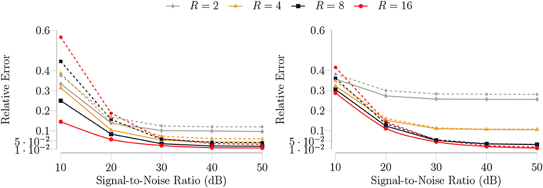
Figure 4. (Left) The median test (dashed lines) and training (solid lines) errors of the type I model for 100 trials on the synthetic noisy data for a rank-8 function given as in Equation (29). The number of samples for the training dataset is set to 5, 000 and for test dataset is set to 1, 000. The batch size is set to 500 and the maximum number of GN iterations is set to 5. (Right) The median test (dashed lines) and training (solid lines) errors of the type II model with the same algorithm settings. TeMPO produces more accurate results and generalizes better for higher rank values for both the type I and type II model in the presence of noise as well. Again, the type I model produces better results for low rank values, i.e., R < R_f, because it involves more parameters than the type II model.

In our next experiment, we trained the type I and type II model with larger-size samples, i.e., N = 250 and R = {8, 16, 32, 64}, to assess how the CPU time depends on the rank. In Figure 5, we show the median CPU time per epoch as a function of the rank. It is evident from the figure that the computational complexity of the type I model is d times the computational complexity of the type II model (cf. Section 3.5). Moreover, Figure 5 confirms that the computational complexity of our algorithm is linear in the rank (cf. Section 3.5).

FIGURE 5

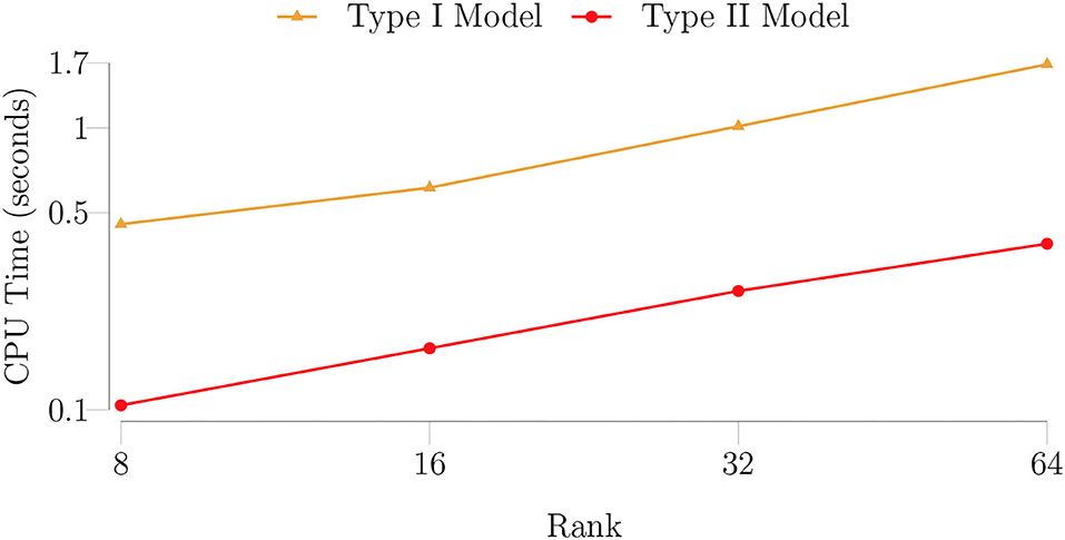
Figure 5. The median CPU time (seconds) per epoch for the type I and type II model as a function of the rank for a rank-8 function given as in Equation (28) for 100 trials. The number of samples for the training dataset is set to 5, 000 and for the test dataset it is set to 1, 000. The batch size is set to 500 and the maximum number of GN iterations is set to 5. The figure confirms that the computational complexity of the type I model is d times the computational complexity of the type II model (cf. Section 3.5). Moreover, the computational complexity of the algorithm is linear in the rank (cf. Section 3.5). The figure is in a logarithmic scale on the horizontal axis.

In our next experiment, we examined the generalization abilities of the Gauss–Newton and ADAM [54] algorithms in our framework. We trained the type I model for a multivariate polynomial of degree 5 with both of these algorithms for different number of training samples to fit the rank-8 function given as in Equation (29). We set R = 8, N = 50, and SNR = 20(dB). For the ADAM algorithm, we set the step size, the exponential decay rate for the first momentum (β₁), and the exponential decay rate for the second momentum (β₂) to 0.01, 0.9, and 0.99, respectively. In Figure 6, we show the median training and test accuracies of these algorithms for the number of training samples ranging from 500 to 5, 000 as a function of the number of epochs for 100 trials. It is evident from Figure 6 that the presented Gauss–Newton algorithm produces more accurate results than the ADAM algorithm and also requires fewer number of epochs to converge in these experimental settings.

FIGURE 6

Figure 6. Comparison of the median test (dashed lines) and training (solid lines) errors of the Gauss–Newton and the ADAM algorithms as a function of the number of epochs for 100 trials. The type I model for a rank-8 function given as in Equation (29) in the presence of SNR 20 dB Gaussian noise is used to generate the training and the test sets. The batch size is set to 10% of the training set size. For the Gauss–Newton algorithm, the maximum number of GN iterations and CG iterations is set to 1 and 5, respectively. For the ADAM algorithm, the step size, β₁ and β₂ are set to 0.01, 0.9, and 0.99, respectively. The number of training samples is set to 500 (top-left), 1, 000 (top-right), 2, 000 (bottom-left), and 5, 000 (bottom-right). The presented Gauss–Newton algorithm produces more accurate results than the ADAM algorithm and also requires fewer number of epochs to converge in these experimental settings.

We also compared TeMPO with SVMs using a polynomial kernel. We run the same experiment for a number of training samples ranging from 500 to 5, 000. We set the rank to 8, i.e., R = R_f for TeMPO. We used the built-in Matlab routine fitrsvm and LS-SVMlab toolbox [55, 56]. We set the degree of polynomial kernel to 5, i.e., equal to the degree of the type I and type II model for fitrsvm. LS-SVMlab automatically tunes the degree to 3 to find the best fit. In Figure 7 (left), we show the median test and training errors for SVM, the type I and type II model. It is clear from Figure 7 (left) that the type I and type II model generalize better than fitrsvm. A possible reason is the dense parameterization of SVMs, while TeMPO uses low-rank parameterization. Moreover, as shown in Figure 7 (right), our algorithm is faster than SVMs for numbers of training samples above 1, 000. This is due to the higher memory requirement of SVMs. Typically, kernel based methods such as LS-SVM have a storage and computational complexity of ${O}(N^2)$ [55], with N the number of training samples. In contrast, Figure 7 (right) confirms that the computational complexity of TeMPO is linear in the number of training samples (cf. Section 3.5).

FIGURE 7

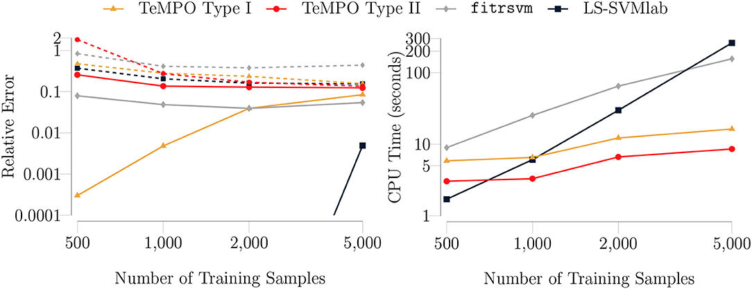
Figure 7. (Left) The median test (dashed lines) and training (solid lines) errors of SVMs with polynomial kernel, the type I and type II model for a rank-8 function given as in Equation (29) in the presence of SNR 20 dB Gaussian noise as a function of the number of training samples for 100 trials. The batch size is equal to 10% of the training set size. The maximum number of GN iterations is set to 5 for the type I and type II model. Specifically, for the SVMs, the built-in Matlab routine fitrsvm and LS-SVMlab toolbox were used to obtain the results. The relative errors of LS-SVMLab for the sample sizes 500, 1, 000, and 2, 000 are 1.6e − 6, 2.2e − 6 and 3.3e − 6, respectively. The presented algorithm generalizes better than fitrsvm in these experimental settings. (Right) The median CPU times (seconds) with the same setting. The computational complexity of our algorithm is linear in the problem size as expected, and it is faster than SVMs for numbers of training samples above 1, 000. The figures are in a logarithmic scale on both the horizontal and vertical axes.

4.2. Blind Deconvolution of Constant Modulus Signals

Blind deconvolution can be formulated as a multivariate polynomial optimization (MPO) problem and hence it fits into the TeMPO framework [15]. In this illustrative example, we limit ourselves to an autoregressive single-input single-output (SISO) system [57], given by

$\begin{array}{ll}{\displaystyle \sum _{l=0}^L}{w}_l·y\left[k-l\right]=s\left[k\right]+n\left[k\right],\text{for}k=1,\dots ,K,& (30)\end{array}$

where y[k], s[k], and n[k] are the measured output signal, the input signal and the noise at the kth measurement, respectively, and w_l denotes the lth filter coefficient. Ignoring the noise for the ease of derivation, (30) can be written as:

$\begin{array}{ll}{Y}^{\text{T}}w=s,& (31)\end{array}$

where Y ∈ ℂ^L×K is a Toeplitz matrix and its rows are the subsequent observations under the assumption that we have K + L − 1 samples y[−L + 1], …, y[K]. The vector $w\in {𝕂}^L$ contains the filter coefficients and the kth entry of the source vector $s\in {ℂ}^K$ is the input signal at the kth time instance, i.e., s_k = s[k]. In blind deconvolution, one attempts to find the original input signal $s$ and the filter coefficients $w$ by only observing the output signal Y. Thus, constraints on signals and/or channel have to be imposed to obtain interpretable results. The constant modulus (CM) criterion is a widely used input constraint [58]. The CM property, which holds for phase- or frequency-modulated signals [50, 59] can be written as:

$\begin{array}{ll}|s_k{|}^2=c,\text{for}k=1,2,\dots ,K.& (32)\end{array}$

Here, c is a constant scalar. By substituting s_k defined in (31) into (32), we obtain

$\begin{array}{ll}{(Y\odot \overline{Y})}^{\text{T}}(w\otimes \overline{w})=c·1_K.& (33)\end{array}$

Following the same intuition as in [60], by multiplying (33) from the left with a Householder reflector Q [61], generated for c·1_K, and removing the first equation³, we obtain

$\begin{array}{ll}M(w\otimes \overline{w})=0.& (34)\end{array}$

Here, $\text{M}=\tilde{\text{Q}}{(\text{Y}\odot \overline{\text{Y}})}^{\mathrm{\text{T}}}$, and $\tilde{\text{Q}}$ is obtained by removing the first row of the Householder reflector Q. In applications, $\text{M}(w\otimes \overline{w})$ will not vanish exactly due to the presence of noise. Hence, we look for the solution which minimizes its l₂ norm as

$\begin{array}{ll}{\displaystyle \underset{w,\overline{w}}{min}}f(w,\overline{w})={\displaystyle \underset{w,\overline{w}}{min}}\frac{1}{2}\left|\right|M(w\otimes \overline{w})|{|}_2^2,\text{subject to}|\left|w\right||=1.& (35)\end{array}$

The objective function in (35) is a homogeneous multivariate polynomial of degree 4 in which the coefficient tensor ${W}$ is given as a rank-1 Hermitian symmetric CPD, i.e.,

$\begin{array}{ll}{W}=w\otimes \overline{w}\otimes \overline{w}\otimes w:=w,\overline{w},\overline{w},w.& (36)\end{array}$

Exploiting the rank-1 Hermitian symmetric CPD structure in (36) and the structure of M, which is a special case of Lemma 1 and Lemma 2, efficient expressions for the computation of Jacobian-vector products for the problem (35) have been presented in [15].

A number of algorithms have been developed to solve (33) and (34). The analytical CM algorithm (ACMA) [50] writes (34) as a generalized matrix eigenvalue problem in the absence of noise, and under the assumption that the null space of M is one dimensional, which makes ACMA more restrictive than TeMPO. In the presence of noise, ACMA writes (34) as the simultaneous diagonalization of a number of matrices and solves it by extended QZ iteration. Gradient descent and stochastic gradient descent algorithms have also been proposed for the minimization of the expected value of $\left\{{(|y_n^{\mathrm{\text{T}}}w|-c)}^2\right\}$. The optimal step-size CMA (OSCMA) [51] algorithm uses a gradient descent algorithm, which computes the step size algebraically. The problem in (35) can also be interpreted as a linear system with a rank-1 constrained solution, which fits the LS-CPD framework in [52]. LS-CPD solves (33) by relaxing the complex conjugate $\overline{w}$ to a possibly different vector $v\in {ℂ}^L$ and utilizing the second-order GN algorithm using dogleg trust-region method. We solve (35) by utilizing the complex GN algorithm using the conjugate gradient Steihaug method implemented in TensorLab 3.0 [11]. We compare with these algorithms in terms of computation time and accuracy.

We consider an autoregressive model of degree L = 10 with coefficients uniformly distributed on [0, 1], sample length K = 600, and c = 1. We add scaled Gaussian noise to the measurements to obtain a particular SNR. We run 50 experiments starting from the algebraic solution presented in [52] for LS-CPD, OSCMA, and TeMPO. In Figure 8 (left), we show the median relative error on $w$ as a function of SNR. It is clear from Figure 8 (left) that TeMPO achieves similar accuracy as LS-CPD and OS-CMA, which are more accurate than ACMA. In Figure 8 (right), we show the median CPU time in seconds as a function of SNR. Clearly, TeMPO is faster than ACMA, OS-CMA, and LS-CPD for SNR ≥ 10(dB) by exploiting the structure of the data.

FIGURE 8

Figure 8. (Left) The median relative errors (dB) of LS-CPD, OS-ACMA, ACMA, and TeMPO with respect to SNR (dB) for an autoregressive model of degree L = 10 with uniformly distributed coefficients between zero and one, sample length K = 600 for 50 trials. TeMPO obtains similar accuracy to LS-CPD, OS-CMA, while obtaining more accurate results than ACMA. (Right) The median CPU times (seconds) with the same settings. TeMPO is faster than other algorithms for SNR > 10 (dB).

4.3. Image Classification

Multi-class image classification amounts to the determination of a possibly nonlinear function f that maps input images Z_k to integer scalar labels y_k, which are known for a training set. In this study, we represent f by a multivariate polynomial p. Following the one-versus-all strategy, we define a cost function f_l for each label that maps the input image Z_k to a scalar value as

$\begin{array}{l}{f}_l(p_l,z_1,\dots ,z_K)=\frac{1}{2}{\displaystyle \sum _{k=1}^K}{(y_k-p_l(z_k))}^2,\end{array}$

where $z_k=\mathrm{\text{vec}}({\text{Z}}_k)$ and where y_k = 1 if $z_k$ is labeled as l and y_k = 0 otherwise. The polynomial p_l can be chosen within the type I or the type II model class. For the type I model, the optimization problem can be written as

$\begin{array}{l}{\displaystyle \underset{p_l}{min}}{f}_l(p_l,z_1,\dots ,z_K),\text{subject to}{p}_l(z_k)={{T}}_{l,0}+{\displaystyle \sum _{j=1}^d}{{T}}_{l,j}{z}_k^j,\\ \text{ and}{{T}}_{l,j}=U_{l,j},\dots ,U_{l,j};c_{l,j}^{\text{T}},& (37)\end{array}$

where d is the degree of the polynomial under consideration. Note that we substitute the symmetric CPD structure given as a constraint into the objective function, and hence obtain and solve an unconstrained optimization problem. For the type II model, the optimization problem can be written as

$\begin{array}{l}{\displaystyle \underset{p_l}{min}}{f}_l(p_l,z_1,\dots ,z_K),\text{subject to}{p}_l(z_k)={{T}}_l{z}_k^d,\\ \text{ and}{{T}}_l=〚U_l,\dots ,U_l;c_l^{\text{T}}〛.\end{array}$

After the optimization of f_l for each label l, the classification is done by computing each $p_l(s)$ for the data point $s$ to be classified and selecting the value of l for which $\left|p_l(s)\right|$ is largest.

4.3.1. Experiments

We performed several experiments by varying the parameters rank and maximum number of GN iterations to illustrate the TeMPO framework for the classification of the MNIST and Fashion MNIST datasets. We kept the maximum number of CG iterations equal to 10, the degree of the multivariate polynomial to 3, the tolerance for the objective function and optimization variables equal to 1e − 10, the inner solver tolerance equal to 1e − 10, and the trust-region radius equal to 0.1, throughout the experiments.

We initialized each factor matrix with a matrix whose elements were randomly drawn from the standard normal distribution, and scaled it to unit norm. Similarly, we initialized each weight vector $c_l$ with a vector whose elements were randomly drawn from the standard normal distribution and scaled it to unit norm.

Datasets

Modified National Institute of Standards and Technology (MNIST) handwritten digit database [62] and the Fashion MNIST database [63] are used for this study. Both datasets contain gray scale images of size (28 × 28). The training sets of both datasets are composed of 60, 000 images and test sets are composed of 10, 000 images. The images have been size-normalized and centered in a fixed-size image. We rescale images such that every pixel value is in the interval [0, 1] and the mean of each image is zero. Then, we vectorize, i.e., stack each column vertically in a vector, each image to a vector of size 784. For the type II model, we augment the resulting vector by the scalar 1. Similar pre-processing steps are necessary for also tensor networks. Additionally, they may require the encoding input data which increases the storage and the computational resource requirement.

Results and Comparisons

Results of the Type I Model

We first trained the type I model on the total MNIST training set for various rank values ranging from 10 to 150 to illustrate the effect of rank on the accuracy. We set the batch size to 100 and the maximum number of GN iterations to 1. We show the training history in Figure 9. It is evident from Figure 9 that TeMPO achieves high accuracy even for low rank values, i.e., R = {10, 20}. Increasing the rank mildly improves both the test and training accuracy, with the improvement getting smaller as the rank increases.

FIGURE 9

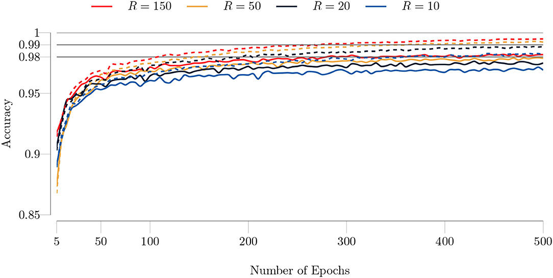
Figure 9. Test (solid lines) and training (dashed lines) accuracies of the type I model for the MNIST dataset with respect to the number of epochs. The full training set (60, 000 images) and test set (10, 000 images) are used. The batch size is set to 100 and the maximum number of GN iterations is set to 1. TeMPO achieves high accuracy even for low rank values, i.e., R = {10, 20}. Both the test and training accuracy increase mildly as the rank increases.

We repeated the same experiments for the Fashion MNIST dataset, which is harder to classify. We show the training history in Figure 10. The observations made for the MNIST dataset also apply to the Fashion MNIST dataset. However, the test and training accuracy are lower for the Fashion MNIST dataset in agreement with previous works. Also, our algorithm requires more epochs to converge for the Fashion MNIST dataset.

FIGURE 10

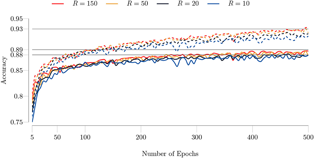
Figure 10. Test (solid lines) and training (dashed lines) accuracies of the type I model for the Fashion MNIST dataset with respect to the number of epochs. The full training set (60, 000 images) and test set (10, 000 images) are used. The batch size is set to 100 and the maximum number of GN iterations is set to 1. Similar to the MNIST dataset, TeMPO achieves good accuracy even for low rank values and both the test and training accuracy mildly increase as the rank increases.

In our next experiment, we set the maximum number of GN iterations to 5. We observed that our algorithm needs fewer epochs to converge and produces more accurate results with this setting. The comparison for the MNIST and Fashion MNIST dataset is shown in Figures 11, 12, respectively. The improvement in the test accuracy for the Fashion MNIST dataset is around 1% and more pronounced than the improvement in the test accuracy for the MNIST dataset. TeMPO achieves around 98.30% test accuracy for the MNIST dataset and around 90% test accuracy for the Fashion MNIST dataset with R = 150.

FIGURE 11

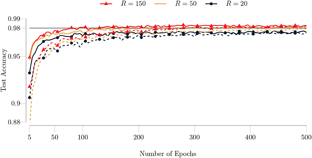
Figure 11. Comparison of test accuracies of the type I model on the MNIST dataset for different maximum number of GN iterations as a function of the number of epochs. The full training set (60, 000 images) and test set (10, 000 images) are used. The batch size is set to 100 and the maximum number of GN iterations is set to 1 (dashed lines) and to 5 (solid lines).

FIGURE 12

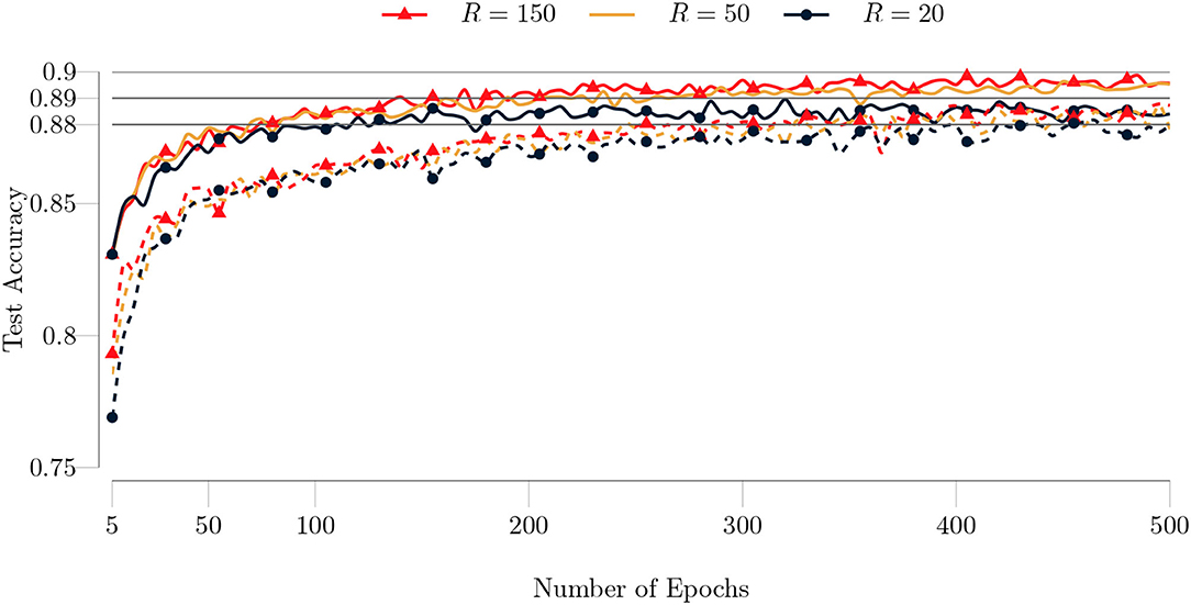
Figure 12. Comparison of test accuracies of the type I model on the Fashion MNIST dataset for different maximum number of GN iterations as a function of the number of epochs. The full training set (60, 000 images) and test set (10, 000 images) are used. The batch size is set to 100 and the maximum number of GN iterations is set to 1 (dashed lines) and to 5 (solid lines).

Results of the Type II Model

We repeated the same experiments for the type II model. We used the same settings as in the type I model. However, we set the batch size to 200 to obtain an accuracy similar to that of the type I model. We show the training history in Figure 13. Similar to previous experiments, our algorithm performs well even for low rank values, and produces more accurate results for higher rank values. TeMPO achieves around 98% test accuracy and 100% training accuracy after 200 epochs with R = 150 for the MNIST dataset.

FIGURE 13

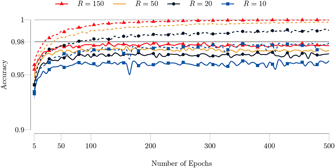
Figure 13. Test (solid lines) and training (dashed lines) accuracies of the type II model for the MNIST dataset with respect to the number of epochs. The full training set (60, 000 images) and test set (10, 000 images) are used. The batch size is set to 200 and the maximum number of GN iterations is set to 1. Both the test and training accuracy increase as the rank increases. The improvement in the accuracy gets smaller as the rank increases. The algorithm achieves around 100% training accuracy after 200 epochs.

In Figure 14, we show the training history for the Fashion MNIST dataset. Similar to the type I model, the test and training accuracy is lower than the MNIST dataset. The algorithm converges around 100 epochs and achieves around 89.30% test accuracy with R = 150. Moreover, our algorithm achieves around 99% training accuracy after 400 epochs.

FIGURE 14

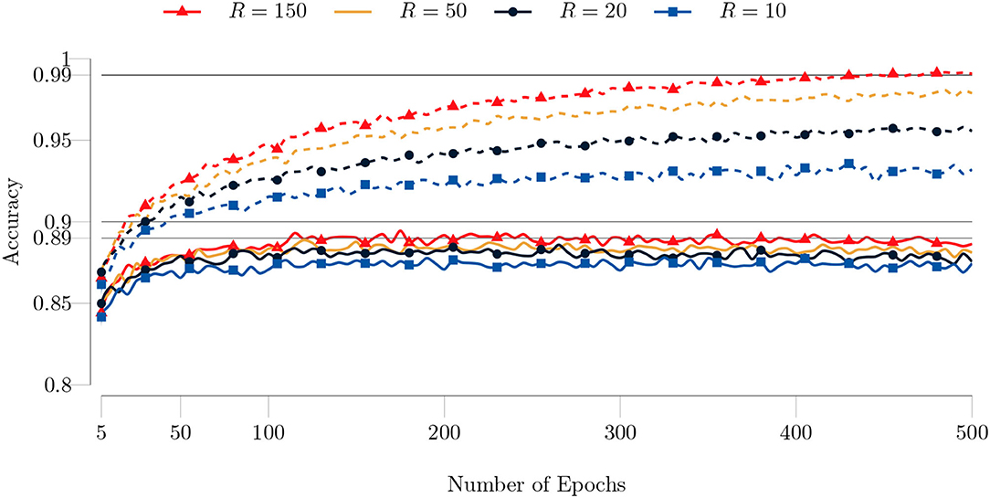
Figure 14. Test (solid lines) and training (dashed lines) accuracies of the type I model for the MNIST dataset with respect to the number of epochs. The full training set (60, 000 images) and test set (10, 000 images) are used. The batch size is set to 200 and the maximum number of GN iterations is set to 1. Both the test and training accuracy increase as the rank increases. Also the improvement in the accuracy gets smaller as the rank increases. The algorithm achieves around 99% training accuracy after 400 epochs.

We repeated the same experiments with the maximum number of GN iterations set to 5. The comparisons for the MNIST and Fashion MNIST datasets are shown in Figure 15. Contrary to our observation for the type I model, the test accuracy now decreases for both datasets. A possible reason is that when the residuals are big, doing more GN iterations may not lead a better direction for minimizing (37). A similar observation has been made in [53], for training DNNs. It is experimentally shown that higher number of CG iterations might not produce more accurate results if the Hessian obtained by mini-batch is not reliable due to non-representative batches and/or big residuals. On the other hand, if the residuals are small, higher number of CG iterations can produce more accurate results thanks to the curvature information [53].

FIGURE 15

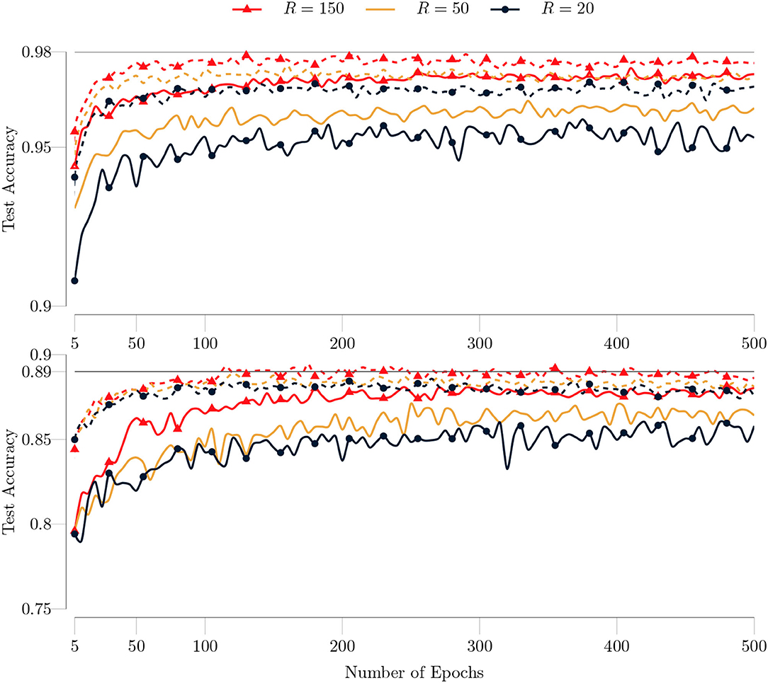
Figure 15. Comparison of test accuracies of the type II model on the MNIST (top) and Fashion MNIST (bottom) datasets for different maximum number of GN iterations as a function of the number of epochs. The full training set (60, 000 images) and test set (10, 000 images) are used. The batch size is set to 200 and the maximum number of GN iterations is set to 1 (dashed lines) and to 5 (solid lines).

Comparisons

We now compare TeMPO with different models, namely: TT tensor networks [21], TT structured tree tensor networks (TTN) [64], multi-layer perceptron (MLP) with 784−1000−10 neurons, MLP with a convolution layer (CNN-MLP), PEPS, and PEPS with a convolution layer (CNN-PEPS) [22]. We compare in terms of the test accuracy for the Fashion MNIST dataset. We summarize the test accuracy of different models in Table 2. TeMPO achieves better accuracy than TT, PEPS and MLP, while optimizing for fewer parameters and using less memory (cf. Table 1). The accuracy of TeMPO is lower than CNN-MLP and CNN-PEPS as expected, since it does not use a convolution layer. Note that the accuracy of TeMPO can further be improved by tuning the parameters such as the rank, the number of CG iterations, the trust-region radius, the batch size and the degree of the multivariate polynomial.

TABLE 2

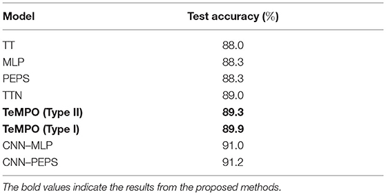
Table 2. The test accuracy of different models for the Fashion MNIST dataset.

5. Conclusion and Future Work

We presented the TeMPO framework for use in nonlinear optimization problems arising in signal processing, machine learning, and artificial intelligence. We modeled the nonlinearities in these problems by multivariate polynomials represented by low rank tensors. In particular, we investigated the symmetric CPD format in this study. By taking the advantage of low rank symmetric CPD structure, we developed an efficient second-order batch Gauss–Newton algorithm. We demonstrated the efficiency of TeMPO with some illustrative examples, and with the blind deconvolution of constant modulus signals. We showed that TeMPO achieves similar or better classification rates than MLPs, TT and PEPS tensor networks on the MNIST and Fashion MNIST datasets while optimizing for fewer parameters and using less memory space.

The non-symmetric and partially symmetric CPD formats are fairly straightforward variants of the symmetric CPD format in which the factor matrices can be mutually different. Efficient algorithms can be developed for multivariate polynomials in these formats by utilizing the derivations presented in this study. We are investigating other tensor formats such as HT and TT in our framework as well. HT and TT require more parameters than the CPD format. However, they break the curse of dimensionality in a numerically stable way. We are also exploring other polynomial bases, and more generally other nonlinear feature maps to further improve the accuracy and numerical stability of our framework.

Data Availability Statement

Publicly available datasets were analyzed in this study. This data can be found at: http://yann.lecun.com/exdb/mnist/; https://github.com/zalandoresearch/fashion-mnist.

Author Contributions

MA developed the theory and Matlab implementation. He is the main contributor to the numerical experiments and also wrote the first draft of the manuscript. LD conceived the idea and supervised the project. Both authors contributed to manuscript revision, read, and approved the submitted version.

Funding

Research supported by: (1) Flemish Government: This research received funding from the Flemish Government (AI Research Program). LD and MA are affiliated to Leuven. AI-KU Leuven institute for AI, B-3000, Leuven, Belgium. This work was supported by the Fonds de la Recherche Scientifique – FNRS and the Fonds Wetenschappelijk Onderzoek – Vlaanderen under EOS Project no G0F6718N (SeLMA). (2) KU Leuven Internal Funds: C16/15/059, IDN/19/014.

Conflict of Interest

The authors declare that the research was conducted in the absence of any commercial or financial relationships that could be construed as a potential conflict ofinterest.

Publisher's Note

All claims expressed in this article are solely those of the authors and do not necessarily represent those of their affiliated organizations, or those of the publisher, the editors and the reviewers. Any product that may be evaluated in this article, or claim that may be made by its manufacturer, is not guaranteed or endorsed by the publisher.

Acknowledgments

The authors would like to thank E. Evert, N. Govindarajan, and S. Hendrikx for proofreading the manuscript and N. Vervliet for valuable discussions. The authors also thank the two referees whose comments/suggestions helped improve and clarify this manuscript.

Footnotes

1. ^Since the weight vector $c$ is used in the parametrization of tensors, different choices of constant in $\tilde{z}$ lead to mathematically equivalent cost functions in the optimization problems. On the other hand, the choice of the constant may imply numerical differences—in situations of this type, one should generally choose a constant that “makes sense for the application.”

2. ^Note that the non-symmetric and partially symmetric CPD formats are fairly straightforward variants of the symmetric CPD format, and derivations presented in Section 3.4 can be generalized to these formats with slight modifications.

3. ^The first equation is only a normalization constraint.

References

1. Sidiropoulos N, De Lathauwer L, Fu X, Huang K, Papalexakis EE, Faloutsos C. Tensor decomposition for signal processing and machine learning. IEEE Trans Signal Process. (2017) 65:3551–82. doi: 10.1109/TSP.2017.2690524

CrossRef Full Text | Google Scholar

2. Cichocki A, Mandic DP, De Lathauwer L, Zhou G, Zhao Q, Caiafa CF, et al. Tensor decompositions for signal processing applications: from two-way to multiway component analysis. IEEE Signal Process Mag. (2015) 32:145–63. doi: 10.1109/MSP.2013.2297439

CrossRef Full Text | Google Scholar

3. Kolda TG, Bader BW. Tensor decompositions and applications. SIAM Rev. (2009) 51:455–500. doi: 10.1137/07070111X

CrossRef Full Text | Google Scholar

4. Sorber L, Van Barel M, De Lathauwer L. Optimization-based algorithms for tensor decompositions: Canonical polyadic decomposition, decomposition in rank-(L_r, L_r, 1) terms, and a new generalization. SIAM J Optim. (2013) 23:695–720. doi: 10.1137/120868323

CrossRef Full Text | Google Scholar

5. Sorber L, Van Barel M, De Lathauwer L. Unconstrained optimization of real functions in complex variables. SIAM J Optim. (2012) 22:879–98. doi: 10.1137/110832124

CrossRef Full Text | Google Scholar

6. Vervliet N, De Lathauwer L. Numerical optimization based algorithms for data fusion. In: Cocchi M, editor. Data Fusion Methodology and Applications. Vol. 31. Amsterdam; Oxford; Cambridge: Elsevier (2019). p. 81–128. doi: 10.1016/B978-0-444-63984-4.00004-1

CrossRef Full Text | Google Scholar

7. Phan AH, Tichavský P, Cichocki A. Low Complexity Damped Gauss-Newton Algorithms for CANDECOMP/PARAFAC. arXiv:1205.2584. (2013) 34:126–47. doi: 10.1137/100808034

CrossRef Full Text | Google Scholar

8. Vervliet N, De Lathauwer L. A randomized block sampling approach to canonical polyadic decomposition of large-scale tensors. IEEE J Selec Top Sign Process. (2016) 10:284–95. doi: 10.1109/JSTSP.2015.2503260

CrossRef Full Text | Google Scholar

9. Comon P, Jutten C. Handbook of Blind Source Separation: Independent Component Analysis and Applications. Oxford; Burlington: Academic Press; Elsevier (2009).

Google Scholar

10. Vervliet N, Debals O, Sorber L, De Lathauwer L. Breaking the curse of dimensionality using decompositions of incomplete tensors: tensor-based scientific computing in big data analysis. IEEE Signal Process Mag. (2014) 31:71–9. doi: 10.1109/MSP.2014.2329429

CrossRef Full Text | Google Scholar

11. Vervliet N, Debals O, Sorber L, Van Barel M, De Lathauwer L. Tensorlab 3.0. (2016). Available online at https://www.tensorlab.net (accessed December, 2021).

Google Scholar

12. Vervliet N. Compressed Sensing Approaches to Large-Scale Tensor Decompositions. Leuven: KU Leuven (2018).

Google Scholar

13. Vandecappelle M, Vervliet N, Lathauwer LD. Inexact generalized gauss-newton for scaling the canonical polyadic decomposition with non-least-squares cost functions. IEEE J Selec Top Sign Process. (2021) 15:491–505. doi: 10.1109/JSTSP.2020.3045911

CrossRef Full Text | Google Scholar

14. Singh N, Zhang Z, Wu X, Zhang N, Zhang S, Solomonik E. Distributed-memory tensor completion for generalized loss functions in python using new sparse tensor kernels. arXiv:191002371. (2021). doi: 10.48550/arXiv.1910.02371

CrossRef Full Text | Google Scholar

15. Ayvaz M, De Lathauwer L. Tensor-based multivariate polynomial optimization with application in blind identification. In: (2021) 29th Europian Signal Processing Conference, (EUSIPCO). Dublin (2021). p. 1080–4. doi: 10.23919/EUSIPCO54536.2021.9616070

CrossRef Full Text | Google Scholar

16. Grasedyck L, Kressner D, Tobler C. A literature survey of low-rank tensor approximation techniques. GAMM-Mitteil. (2013) 36:53–78. doi: 10.1002/gamm.201310004

CrossRef Full Text | Google Scholar

17. Grasedyck L. Hierarchical singular value decomposition of tensors. SIAM J Matrix Anal Appl. (2010) 31:2029–54. doi: 10.1137/090764189

CrossRef Full Text | Google Scholar

18. Oseledets IV, Tyrtyshnikov EE. Breaking the curse of dimensionality, or how to use SVD in many dimensions. SIAM J Sci Comput. (2009) 31:3744–59. doi: 10.1137/090748330

CrossRef Full Text | Google Scholar

19. Novikov A, Trofimov M, Oseledets IV. Exponential machines. In: 5th International Conference on Learning Representations, ICLR 2017. Toulon (2017). Available online at: https://openreview.net/forum?id=rkm1sE4tg

Google Scholar

20. Stoudenmire EM, Schwab DJ. Supervised learning with tensor networks. In: Lee D, Sugiyama M, Luxburg U, Guyon I, Garnett R, editors. Advances in Neural Information Processing Systems. Vol. 29. Barcelona: Curran Associates, Inc. (2016). Available online at: https://proceedings.neurips.cc/paper/2016/file/5314b9674c86e3f9d1ba25ef9bb32895-Paper.pdf

Google Scholar

21. Efthymiou S, Hidary J, Leichenauer S. TensorNetwork for machine learning. arXiv: 190606329. (2019). doi: 10.48550/arXiv.1906.06329

CrossRef Full Text | Google Scholar

22. Cheng S, Wang L, Zhang P. Supervised learning with projected entangled pair states. Phys Rev B. (2021) 103:125117. doi: 10.1103/PhysRevB.103.125117

CrossRef Full Text | Google Scholar

23. Guo W, Kotsia I, Patras I. Tensor learning for regression. IEEE Trans Image Process. (2012) 21:816–27. doi: 10.1109/TIP.2011.2165291

PubMed Abstract | CrossRef Full Text | Google Scholar

24. Hendrikx S, Boussé M, Vervliet N, De Lathauwer L. Algebraic and optimization based algorithms for multivariate regression using symmetric tensor decomposition. In: Proceedings of the (2019) IEEE International Workshop on Computational Advances in Multi-Sensor Adaptive Processing (CAMSAP). Guadeloupe (2019). p. 475–9. doi: 10.1109/CAMSAP45676.2019.9022662

PubMed Abstract | CrossRef Full Text | Google Scholar

25. Rabusseau G, Kadri H. Low-rank regression with tensor responses. In: Lee D, Sugiyama M, Luxburg U, Guyon I, Garnett R, editors. Advances in Neural Information Processing Systems. Vol. 29. Barcelona: Curran Associates, Inc. (2016). Available online at: https://proceedings.neurips.cc/paper/2016/file/3806734b256c27e41ec2c6bffa26d9e7-Paper.pdf

PubMed Abstract | Google Scholar

26. Yu R, Liu Y. Learning from multiway data: simple and efficient tensor regression. In: Balcan MF, Weinberger KQ, editors. Proceedings of the 33rd International Conference on Machine Learning, Vol. 48 of Proceedings of Machine Learning Research. New York, NY (2016). p. 373–81. Available online at: https://proceedings.mlr.press/v48/yu16.html

Google Scholar

27. Hou M, Chaib-Draa B. Hierarchical Tucker tensor regression: application to brain imaging data analysis. In: Proceedings of the (2015) IEEE International Conference on Image Processing (ICIP 2015). Québec, QC (2015). p. 1344–8. doi: 10.1109/ICIP.2015.7351019

CrossRef Full Text | Google Scholar

28. Kar P, Karnick H. Random feature maps for dot product kernels. In: Lawrence ND, Girolami M, editors. Proceedings of the Fifteenth International Conference on Artificial Intelligence and Statistics, Vol. 22 of Proceedings of Machine Learning Research. La Palma (2012). p. 583–91. Available online at: https://proceedings.mlr.press/v22/kar12.html

PubMed Abstract | Google Scholar

29. Yang J, Gittens A. Tensor machines for learning target-specific polynomial features. arxiv: 150401697. (2015). doi: 10.48550/arXiv.1504.01697

CrossRef Full Text | Google Scholar

30. Rendle S. Factorization machines. In: (2010) IEEE International Conference on Data Mining. Sydney (2010). p. 995–1000. doi: 10.1109/ICDM.2010.127

CrossRef Full Text | Google Scholar

31. Blondel M, Fujino A, Ueda N, Ishihata M. Higher-order factorization machines. In: Proceedings of the 30th International Conference on Neural Information Processing Systems, NIPS'16. Red Hook, NY: Curran Associates Inc. (2016). p. 3359–67.

Google Scholar

32. Blondel M, Ishihata M, Fujino A, Ueda N. Polynomial networks and factorization machines: new insights and efficient training algorithms. In: Proceedings of the 33rd International Conference on International Conference on Machine Learning. Vol. 48. New York, NY (2016). p. 850–8.

Google Scholar

33. Nocedal J, Wright S. Numerical Optimization. New York, NY: Springer (2006).

Google Scholar

34. Kruskal JB. Three-way arrays: rank and uniqueness of trilinear decompositions, with application to arithmetic complexity and statistics. Linear Algeb Appl. (1977) 18:95–138. doi: 10.1016/0024-3795(77)90069-6

CrossRef Full Text | Google Scholar

35. Sidiropoulos ND, Bro R. On the uniqueness of multilinear decomposition of N-way arrays. J Chemometr. (2000) 14:229–39. doi: 10.1002/1099-128X(200005/06)14:3<229::AID-CEM587>3.0.CO;2-N

CrossRef Full Text | Google Scholar

36. Domanov I, De Lathauwer L. On the uniqueness of the canonical polyadic decomposition of third-order tensors – Part ii: uniqueness of the overall decomposition. SIAM J Matrix Anal Appl. (2013) 34:876–903. doi: 10.1137/120877258

CrossRef Full Text | Google Scholar

37. Domanov I, De Lathauwer L. Canonical polyadic decomposition of third-order tensors: relaxed uniqueness conditions and algebraic algorithm. arXiv:1501.07251. (2017) 513:342–75. doi: 10.1016/j.laa.2016.10.019

CrossRef Full Text | Google Scholar

38. Boyd JP, Ong JR. Exponentially-convergent strategies for defeating the Runge phenomenon for the approximation of non-periodic functions, part I: single-interval schemes. Commun Comput Phys. (2009) 5:484–97.

Google Scholar

39. Trefethen LN. Approximation Theory and Approximation Practice, Extended Edition. Philadelphia, PA: SIAM (2019). doi: 10.1137/1.9781611975949

CrossRef Full Text | Google Scholar

40. De Lathauwer L, De Moor B, Vandewalle J. On the best rank-1 and rank-(R₁, R₂, ⋯ , R_N) approximation of higher-order tensors. SIAM J Matrix Anal Appl. (2000) 21:1324–42. doi: 10.1137/S0895479898346995

CrossRef Full Text | Google Scholar

41. Zhang T, Golub G. Rank-one approximation to high order tensors. SIAM J Matrix Anal Appl. (2001) 23:534–50. doi: 10.1137/S0895479899352045

PubMed Abstract | CrossRef Full Text | Google Scholar

42. Guan Y, Chu MT, Chu D. SVD-based algorithms for the best rank-1 approximation of a symmetric tensor. SIAM J Matrix Anal Appl. (2018) 39:1095–115. doi: 10.1137/17M1136699

CrossRef Full Text | Google Scholar

43. Nie J, Wang L. Semidefinite relaxations for best rank-1 tensor approximations. SIAM J Matrix Anal Appl. (2013) 35:1155–79. doi: 10.1137/130935112

CrossRef Full Text | Google Scholar

44. Brachat J, Comon P, Mourrain B, Tsigaridas E. Symmetric tensor decomposition. Linear Algeb Appl. (2010) 433:1851–72. doi: 10.1016/j.laa.2010.06.046

CrossRef Full Text | Google Scholar

45. Alexander J, Hirschowitz A. Polynomial interpolation in several variables. Adv Comput Math. (1995) 4:201–22.

Google Scholar

46. Debals O. Tensorization and Applications in Blind Source Separation. Leuven: KU Leuven (2017).

Google Scholar

47. Blondel M, Niculae V, Otsuka T, Ueda N. Multi-output Polynomial Networks and Factorization Machines. In: Advances in Neural Information Processing Systems 30: Annual Conference on Neural Information Processing Systems 2017. Long Beach, CA (2017). p. 3349–59.

Google Scholar

48. Khoromskij BN. Tensor Numerical Methods in Scientific Computing. Berlin; Boston: De Gruyter (2018). doi: 10.1515/9783110365917

CrossRef Full Text | Google Scholar

49. Margossian CC. A review of automatic differentiation and its efficient implementation. WIREs Data Mining Knowl Discov. (2019) 9:e1305. doi: 10.1002/widm.1305

CrossRef Full Text | Google Scholar

50. van der Veen AJ, Paulraj A. An analytical constant modulus algorithm. IEEE Trans Signal Process. (1996) 44:1136–55. doi: 10.1109/78.502327

CrossRef Full Text | Google Scholar

51. Zarzoso V, Comon P. Optimal step-size constant modulus algorithm. IEEE Trans Commun. (2008) 56:10–3. doi: 10.1109/TCOMM.2008.050484

CrossRef Full Text | Google Scholar

52. Boussé M, Vervliet N, Domanov I, Debals O, De Lathauwer L. Linear systems with a canonical polyadic decomposition constrained solution: algorithms and applications. Numer Linear Algeb Appl. (2018) 25:e2190. doi: 10.1002/nla.2190

CrossRef Full Text | Google Scholar

53. Gargiani M, Zanelli A, Diehl M, Hutter F. On the promise of the stochastic generalized Gauss-Newton method for training DNNs. arXiv: 200602409. (2020). doi: 10.48550/arXiv.2006.02409

CrossRef Full Text | Google Scholar

54. Kingma DP, Ba J. Adam: a method for stochastic optimization. In: Bengio Y, LeCun Y, editors. International Conference on Learning Representations, ICLR 2015. 3rd Edn. San Diego, CA (2015). Available online at: http://arxiv.org/abs/1412.6980

Google Scholar

55. De Brabanter K, Karsmakers P, Ojeda F, Alzate C, De Brabanter J, Pelckmans K, et al. LS-SVMlab Toolbox User's Guide Version 1.8. Leuven: ESAT-STADIUS (2010). p. 10–46.

Google Scholar

56. Suykens JAK, Van Gestel T, De Brabanter J, De Moor B, Vandewalle J. Least Squares Support Vector Machines. Singapore: World Scientific (2002). doi: 10.1142/5089

CrossRef Full Text | Google Scholar

57. Ljung L. System Identification: Theory for the User. 2nd ed. Upper Saddle River, NJ: Prentice Hall (1999). doi: 10.1002/047134608X.W1046

CrossRef Full Text | Google Scholar

58. Johnson R, Schniter P, Endres TJ, Behm JD, Brown DR, Casas RA. Blind equalization using the constant modulus criterion: a review. Proc IEEE. (1998) 86:1927–50. doi: 10.1109/5.720246

CrossRef Full Text | Google Scholar

59. van der Veen AJ. Algebraic methods for deterministic blind beamforming. Proc IEEE. (1998) 86:1987–2008. doi: 10.1109/5.720249

CrossRef Full Text | Google Scholar

60. De Lathauwer L. Algebraic techniques for the blind deconvolution of Constant Modulus signals. In: Proceedings of the 12th European Signal Processing Conference (EUSIPCO 2004). Vienna (2004). p. 225–8.

Google Scholar

61. Householder AS. Unitary triangularization of a nonsymmetric matrix. J ACM. (1958) 5:339–42. doi: 10.1145/320941.320947

CrossRef Full Text | Google Scholar

62. Deng L. The MNIST database of handwritten digit images for machine learning research. IEEE Sign Process Mag. (2012) 29:141–2. doi: 10.1109/MSP.2012.2211477

CrossRef Full Text | Google Scholar

63. Xiao H, Rasul K, Vollgraf R. Fashion-MNIST: a novel image dataset for benchmarking machine learning algorithms arXiv:1708.07747. (2017). doi: 10.48550/arXiv.1708.07747

CrossRef Full Text | Google Scholar

64. Stoudenmire EM. Learning relevant features of data with multi-scale tensor networks. Quant Sci Technol. (2018) 3:034003. doi: 10.1088/2058-9565/aaba1a

CrossRef Full Text | Google Scholar