A Step Forward to Formalize Tailored to Problem Specificity Mathematical Transforms

Introduction

Tailored to the Problem Specificity Mathematical Transforms (TPS MTs) were defined as extension of linear transforms [1], when orthogonal bases of the classical Fourier or wavelets transforms are replaced by “physiologically plausible,” non-orthogonal, and parametrized bases, more suited to the physiology or physics of the phenomena being modeled, like in a transform called Dynalet, based on the potential Hamiltonian decomposition of Liénard systems [2, 3]. This article is an effort to improve TPS MT formalism. In this sense, it is claimed that because Extreme Learning Machines (ELMs) [4] are implemented in Fast Artificial Neural Network (FANN), with an extremely fast and analytically well-formalized training cycle, we use here FANN in place of backpropagation ANN (BANN) previously used to define TPS MT.

General Description of Tailored to the Problem Specificity Mathematical Transform

Tailored to the Problem Specificity Mathematical Transform will be calculated in this article by using a trained Fast Artificial Neural Network (FANN), which presents a low algorithm complexity as compared, for example, with numerical methods [4]. In Figure 1, (ε₁, ε₂, …, ε_n) corresponds to the i-th input vector of the FANN, whose weight matrices [Ω^h] and [Ω⁰] contain each n columns equal, respectively, to vectors (${\omega }_{\text{i},1}^{\text{h}},\dots ,{\omega }_{\text{i},\text{m}}^{\text{h}}$) and (${\omega }_{\text{i},1}^0,\dots$, ${{\omega }_{\text{i},\text{p}}}^0$).

FIGURE 1

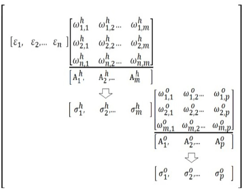
Figure 1. Trained single-layer Artificial Neural Network (ANN) of low complexity to solve Tailored to the Problem Specificity Mathematical Transform (TPS MT) [5].

The vectors (${\omega }_{\text{i},1}^{\text{h}},\dots ,{\omega }_{\text{i},\text{m}}^{\text{h}}$) and (${\omega }_{\text{i},1}^0,\dots$, ${\omega }_{\text{i},\text{p}}^0$) correspond, respectively, to the synaptic coefficients from input to hidden layer and from hidden to output layer matrices; the activation vectors (${\text{A}}_1^{\text{h}},\dots ,A_{\text{m}}^{\text{h}}$) and (${\text{A}}_1^0,\dots ,A_{\text{p}}^0$) are functions of hidden and output neurons and vectors (${\sigma }_m^{\text{h}},\dots ,{\sigma }_m^{\text{h}}$) and (${\sigma }_p^0,\dots ,{\sigma }_p^0$) are the neuron outputs of hidden and output layers. In reference to Figure 1, using ELM within a single-layer FANN and under assumptions, which are discussed in the middle of Section 4 of this article, its training cycle can be reduced to solve the equation:

$\begin{array}{ll}\left[{\Omega }^o\right]={\left[{\Sigma }^h\right]}^{-1}\left[T\right],& (1)\end{array}$

where [Ω^o] is the synaptic weight matrix from hidden to output layer, evidences learning matrix [Σ^h]⁻¹ is the inverse of the Moore–Penrose matrix of the input to hidden layer neurons for each input vector, and [T] is the target matrix, for every input vector. Finally, it is postulated that characterize the above matrices can be dealt with as if they were mathematical transforms between two vector spaces.

Biosignals have been described as being composed by different sequential components that underlie a variety of successive recorded physiological processes: mathematical models of auditory brainstem responses (ABRs), blood pressure waveforms (BPWs), hemodynamic response function (HRF), and homeostatic system dynamics (HSD) will be indeed explored in this article to illustrate TPS, for showing the generic character of our general approach.

Auditory brainstem response in the cat is assumed to be composed by waves originated in the sequential activation of the synaptic relays within the auditory pathway, from cochlear nucleus to cortical projections from the thalamic medial geniculate nucleus to the primary auditory cortical area [5]. ABR has been modeled by 5 sequential components since 1986 [6] up to 2010 [3]. Each of the ABR components is named as a Jewett component (JC). Each JC represents the effect of a global postsynaptic potential in the corresponding relay within the auditory pathway.

Blood pressure waveform in human cardiovascular system is assumed to be composed by up to three or four components [7]. Main component is due to cardiac pumping and it has been confirmed [8] the existence of two major reflection sites in the central arteries. The first occurs in the juncture between thoracic and abdominal aorta and the second occurs in the juncture between abdominal aorta and common iliac arteries. These sites produce the second and third BPW components. Each of the BPW components is named here a Latham component (LC).

Hemodynamic response function is recorded in functional magnetic resonance imaging. When a cortical area is recruited while performing a synchronized motor task, the local oxygen consumption increases, inducing a chain of events, including variations in regional blood volume, blood flow, and relative deoxyhemoglobin/oxyhemoglobin concentration that leads to an increase in the local magnetic resonance signal. It is temporally described by the hemodynamic response function (HRF). The HRF is assumed to be composed by components of a balloon model [9]. The first component corresponds to the inflation phase of the “balloon” representing the local increase in blood volume and the second component corresponds to the deflation phase. Taking into account the elastic properties of the venous compartment and corresponding transient mismatch between variations in local parameters, the balloon model of the HRF is operationally described by two mathematical equations [10, 11], both of them with two components. It is said here that the HRF is composed by Glover component (GC) or Friston component (FC).

Dynalet transform (DT) was defined to represent the HSD. DT produces another example of mathematical transform-based model [3, 12, 13]. It is represented by the general Liénard systems, which obey a non-linear damping equation, generalizing the van der Pol oscillator [14, 15]. Its solution has two components: a Potential (P) and a Hamiltonian (H). DT is said here to be composed by Demongeot components (DCs).

Description of Proposed Transforms

Vector spaces are commonly used to represent mathematical transforms (MTs) in vector spaces (VSs) [1]. In the linear case, however, these structures are restrained to conditions to be accomplished by a subspace to be a basis of MT.

Auditory Brainstem Responses Modeling

Auditory brainstem response has been assumed to be well represented by a linear combination of the first five JCs. Let ABR be the vector subspace of the Banach space of the C_∞ functions defined on R containing the ABRs and a (t) ∈ ABR, approximation in JC model is defined by [3]:

$\begin{array}{ll}\overline{\text{a}}(t)={\displaystyle \sum _{i=1}^5}{c}_i{\text{J}}_i(t),& (2)\end{array}$

where the${\text{J}}_i{(t)}^{\prime }s$, for i equal 1 to 5, are five vectors modeling each JC and c_i is the corresponding i^th coefficient in the linear combination. Each J_i is modeled using the charging dynamics of a pair of leaky electric capacitors circuit (Figure 2) and J_i(t) = J_i (t|α_i, β_i, δ_i) is defined as a single piecewise function like in [16]:

$\begin{array}{r}{\text{J}}_i(t)=\left[e^{-{\alpha }_i(t-{\delta }_i)}-e^{-{\beta }_i(t-{\delta }_i)}\right],fort\ge {\delta }_i\\ {\text{J}}_i(t)=0,fort<{\delta }_i,& (3)\end{array}$

where {(α_i, β_i, δ_i)|i ≤ 5, i ∈ ℕ} is the parameters set of the i^th JC, depending on the electric variables in Figure 2 and estimated to fit data in applications.

FIGURE 2

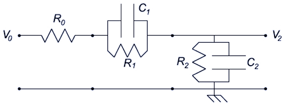
Figure 2. Pair of leaky capacitors analog circuit [16].

Using J_i as basis, the Jewett transform (JT) is defined for an ABR a (t) by:

$\begin{array}{ll}\text{J}(\text{a }(t))\text{=}\left\{(c_i,{\alpha }_i,{\beta }_i,{\delta }_i)|i\le 5,i\in \mathbb{N}\right\}& (4)\end{array}$

The inverse JT converges if J⁻¹oJ$(\text{a }(t))=\overline{\text{a}}(t)\approx \text{a }(t),$where J⁻¹ is the inverse of J. Figure 3 illustrates a reasonably well fit of one ABR with its corresponding model. ABR physiological bases were initially used in [6]. Later, the ANN approach has been proposed to generalize this formalization [3, 16].

FIGURE 3

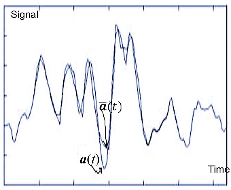
Figure 3. Fitting filtered auditory brainstem response (ABR) a(t) with Artificial Neural Network (ANN) model $\overline{\text{a}}(\mathit{\text{t}})$ [17].

Blood Pressure Waveforms Modeling

The BPW mathematical description has been used in order to develop a non-invasive minimally intrusive (nImI) methodology to estimate blood pressure from pulse waves. Pulse waves were measured using the photoplethysmography (PPG), while the gold standard for BPW is Finapres Nova^® equipment [18]. Initially, phase planes of PPG were recorded in right central finger and in right main toe [19].

Blood pressure waveform is assumed to be well-represented by a linear combination of the first three LCs. Let BPW be the vector space containing every BPW and p (t) ∈ BPW, the LC model can be written [20] as:

$\begin{array}{ll}\overline{p}(t)={\displaystyle {\sum }_{i=1}^3}{c}_i{L}_i(t),& (5)\end{array}$

where the ${\text{L}}_i^{\prime }s$ are three vectors modeling each LC and c_i is the corresponding i^th coefficient in the linear combination. Each L_i is modeled using the solution of a Winkessel (WK) model [21]. In Figure 4, the system WK-4 makes use of four electric elements with an inertia analog to an inductor L, connected in series with the aortic resistance R0. The compliance of the aorta, an analog to a capacitor C, is in parallel with the systemic resistance at the two aortic levels, thoracic (R1) and abdominal (R2), as given in Figure 4 [22].

FIGURE 4

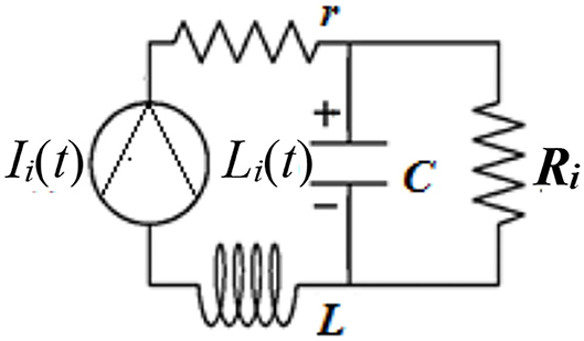
Figure 4. WK-4S analog circuit [22].

The cardiac function can be represented by a current periodic source, with period T_c of the cardiac cycle, which during diastole is off and during systole is given by:

$\begin{array}{ll}\text{I}(t)=I_0{sin}^2({\omega }_{0}t)=I_0(1-cos(2{\omega }_{0}t))/2,& (6)\end{array}$

where ${\omega }_0=\frac{2\pi }{T_s},$with T_s as systolic time duration.

Solving p(t) for each i^th component in the LRC circuit of Figure 4 during the systole, we get for t ≥ δ_i (a time delay), with V_S as the left ventricle stroke volume:

$\begin{array}{l}{\text{L}}_{\text{i}}\left(t\right)=D-K(e^{-\frac{t-{\delta }_i}{{\tau }_i}}\\ -\left(1+\frac{1}{n_i}\right)\left(\frac{cos\left(\frac{2\pi t}{T_s}+{\phi }_i-{\delta }_i\right)}{\sqrt{n_i+1}}+1\right))& (7)\end{array}$

$\begin{array}{ll}\text{where}:K=\frac{V_s{R}_i}{T_s\left(1+\frac{1}{n_i}\right)}& (8)\end{array}$

$\begin{array}{ll}{n}_i={\left(\frac{2\pi {\tau }_i}{T_s}\right)}^2& (9)\end{array}$

$\begin{array}{ll}{\phi }_i={tan}^{-1}\left(\sqrt{n_i}\right)& (10)\end{array}$

$\begin{array}{ll}{\tau }_i{=R}_{i}C& (11)\end{array}$

Then, during the diastolic phase of the cardiac cycle:

$\begin{array}{ll}\{\begin{array}{c}{\text{L}}_i\left(t\right)=D-\frac{V_s{R}_i}{T_s\left(1+\frac{1}{n_i}\right)}\left(e^{-\frac{t-{\delta }_i}{{\tau }_i}}+1\right),fort\ge {\delta }_i\\ {\text{L}}_i\left(t\right)=0,fort<{\delta }_i\\ \end{array}& (12)\end{array}$

Remark that every L_i is zero for t < δ_i and L_i(t) = L_i (t|D, V_s, T_s, T_c, R_i, τ_i, δ_i) for t ≥ δ_i with parameters of the previous heartbeat, where D is the diastolic pressure and T_s and T_c are already defined for the cardiac function as being global parameters applied to the three LCs. WK-4S local parameters for each component are {(R_i, τ_i, δ_i, )|i ≤ 3, i ∈ ℕ)} [22].

Using the ${\text{L}}_i^{\prime }s$ as a basis, Latham transform (LT) is denoted L (b (t)) and is defined for a BPW by:

$\begin{array}{l}\text{L}\left(\text{b}\left(t\right)\right)=\left\{\left(D,V_s,T_s,T_c\right)\cup \left(c_i{,R}_i,{\tau }_i,{\delta }_i\right)|i\le 3,i\in \mathbb{N}\right)\}\end{array}$

The inverse LT converges, if we have:

${\text{L}}^{-1}o\text{L}(\text{b}(t))=\overline{\text{b}}(t)\approx \text{b}(t),$ with L⁻¹ the inverse of L.

Hemodynamic Response Function Modeling

Hemodynamic response function is mathematically described using a balloon model [9]. Two operational representations are explored for this model [10, 11].

The Glover equation assumes that balloon model can be represented by a linear combination of two Glover components (GCs). In this case [23], the corresponding model can be written as:

$\begin{array}{ll}\overline{h}\left(t\right)={\displaystyle {\sum }_{i=1}^2}{c}_i{\text{G}}_i& (13)\end{array}$

where the ${\text{G}}_i^{\prime }s$are two vectors modeling each GC, with G₁ the HRF inflation phase and G₂ the HRF deflation phase, c_i corresponding to the i^th coefficient in the linear combination (c₁ = 1 and c₂ = −c in Glover equation). Each G_i is modeled by:

$\begin{array}{ll}{G}_i\left(t\right)={\text{G}}_{\text{i}}\left(t|{\delta }_i,{\tau }_i\right)={\left(\frac{t}{{\tau }_i}\right)}^{{\delta }_i}{e}^{\left(\left(\frac{{\delta }_i}{{\tau }_i}\right)\left(t-{\tau }_i\right)\right)},& (14)\end{array}$

where {(δ_i, τ_i)|i ≤ 2, i ∈ ℕ)} is the set of the i^ith GC parameters of the Glover model.

Figure 5 illustrates actual HRF superimposed with Glover transform and Levenberg–Marquardt Algorithm (LMA) model [23]. Figure illustrates HRF in a healthy volunteer (blue trace), recorded under informed consent, superimposed with the HRF model estimated using Levenberg–Marquardt Algorithm (LMA) (red trace) and HRF Glover model estimated using TPS MT (green trace), when a conventional Backpropagation Artificial Neural Network is used [23].

FIGURE 5

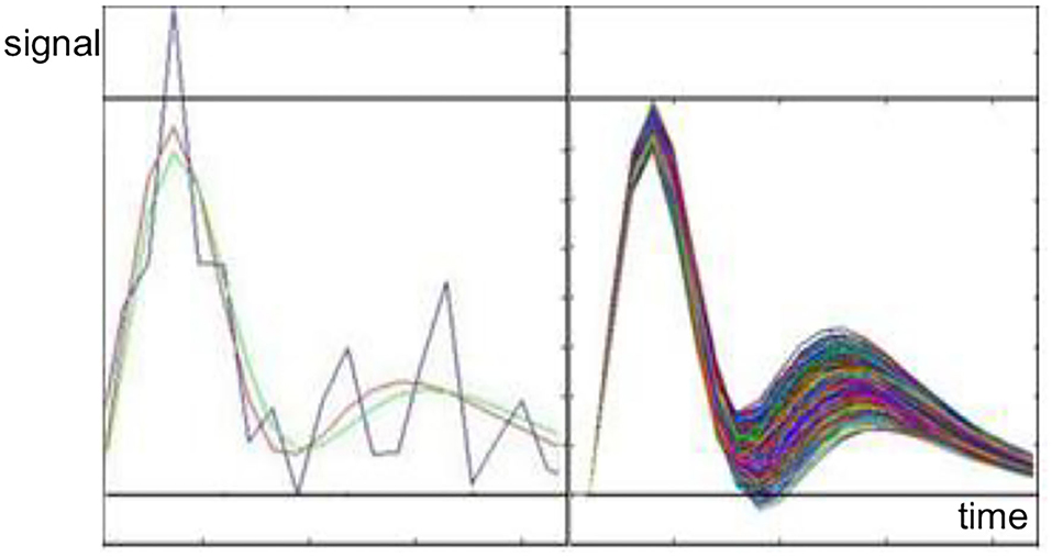
Figure 5. Left: An example of hemodynamic response function (HRF) (black) fitting using Glover transform (GT) (violet) and Levenberg–Marquardt Algorithm (LMA) (green). Right: Inverse GT for different measures (color code in the text).

Although not tested, ELM in the place of backpropagation should produce similar results.

Using the ${\text{G}}_i^{\prime }s$ as a basis, Glover transform (GT) can be defined. If G (h(t)) denotes the GT of a HRF, then G(h(t))= {(c_i, δ_i, τ_i)|i ≤ 2, i ∈ ℕ)}. It is said that the inverse of direct GT converges if GT of h(t) verifies that: ${\text{G}}^{-1}\text{o}\text{G}(\text{h}(t))=\overline{\text{h}}(t)\approx \text{h}(t).$

On another hand, the Friston equation assumes that the Balloon model can be represented by a linear combination of two, so called, Friston components (FCs). If h(t) ∈ HRF, Friston model could be written:

$\begin{array}{ll}\overline{h}\left(t\right)={\displaystyle \sum _{i=1}^2}{c}_i{F}_i\left(t\right),& (15)\end{array}$

where the ${\text{F}}_i^{\prime }s$are two vectors modeling each FC, F₁ is the HRF inflation phase and F₂ is the HRF deflation phase and c_i is the corresponding i^th coefficient in the linear combination (c₁ = A and c₂ = −Ac in Friston equation). Each F_i is modeled as:

$\begin{array}{ll}{F}_i\left(t\right)=F_i\left(t|{\alpha }_i,{\beta }_i\right)=t^{\left({\alpha }_i-1\right)}{\beta }_i^{{\alpha }_i}{e}^{-{\beta }_{i}t}/\Gamma \left({\alpha }_i\right)& (16)\end{array}$

In addition, {(α_i, β_i)|i ≤ 2, i ∈ ℕ)} is the set of the FC parameters of the model.

Using the ${\text{F}}_i^{\prime }s$ as a basis, the Friston transform (FrT) can be defined. The FrT of a HRF h(t) can be written Fr(h(t))= {(c_iα_i, β_i)|i ≤ 2, i ∈ ℕ)}. It could be said that if ${\text{F}\text{r}}^{-1}\text{o}\text{F}\text{r}(\text{h}(t))=\overline{\text{h}}(t)\approx \text{h}(t),$ Fr⁻¹ being the inverse of Fr, then inverse FrT converges.

In this study, GT was used instead of FrT.

Homeostatic System Dynamics Modeling

Dynalet was conceived to represent homeostasis regulation and is based upon Liénard systems decomposition [2]. These systems are second-order differential equation systems, such that:

$\begin{array}{ll}\frac{dx}{dt}=yand\frac{dy}{dt}=Q\left(x\right)+R\left(x\right)y,& (17)\end{array}$

where Q and R are polynomials, e.g., for the van der Pol oscillator [24]:

$\begin{array}{ll}\frac{dx}{dt}=yand\frac{dy}{dt}=-{\omega }^{2}x+\mu \left(1-\frac{x^2}{b^2}\right)y& (18)\end{array}$

This system has been proposed first to model heart activity thanks to its feedback anharmonic term $\mu \left(1-\frac{x^2}{b^2}\right)y$ [15]. There is no algebraic solution to (18), so Hodge decomposition [25] in regular vector space was used to give a family of approximated explicit solutions to any Liénard system by making explicit polynomial approximations of its potential, P, and its Hamiltonian, H, [2, 12, 13, 25–27], which are related to polynomials Q and R, complying:

$\begin{array}{ll}\frac{dx}{dt}=-\frac{\partial P}{\partial x}+\frac{\partial H}{\partial y}and\frac{\partial y}{\partial t}=-\frac{\partial P}{\partial y}-\frac{\partial H}{\partial x}& (19)\end{array}$

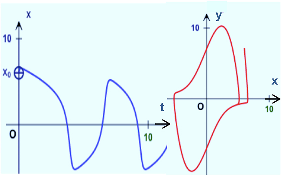
Analogic computing methods were used later to simulate Equation (18) [28]. Figure 6 illustrates this approach. The limit cycle (in blue) corresponds to the stationary homeostatic cycle of the van der Pol oscillator. It is a contour line of the Hamiltonian H. Perturbations from the limit cycle, chosen as initial trajectory, push the dynamics away from the Hamiltonian behavior, the return to it following gradient dynamics with potential P.

FIGURE 6

Figure 6. Solution of (18) with ω = 1, μ = 3, b = 2.6 [28, 29].

The family D of approximate Liénard solutions has a non-orthogonal basis of Demongeot components (DCs). D_i and each solution d(t) can be approximated (for the L2 norm) by Equation (19):

$\begin{array}{ll}d\left(t\right)={\displaystyle \sum _{i=1}^n}{c}_i{D}_i\left(t\right)& (20)\end{array}$

where the ${\text{D}}_i{(t)}^{\prime }s$are given in [2, 12, 13]. They correspond to relaxation dynamical systems whose periods are submultiples of the fundamental period T of the limit cycle of the Liénard system, unique in the van der Pol case. In this last case, the van der Pol oscillator models the cardiac homeostatic regulation [14, 15]. c_i is the corresponding i^th coefficient in the linear combination (20), where n depends on the approximation precision.

Mathematical Transforms

In opposition with linear analysis, where orthogonal basis is used because of mathematical convenience, TPS MT emphasizes the “physiological plausibility” of the modeling approach. In order to evaluate the impact of levering constraints for vectors considered as physiologically plausible, as being part of basis B, the general linear analysis is briefly visited and breakpoints are established providing TPS formalization. Whether V is ABR, BPW, HFR, or HDS, linear combination of physiologically plausible elements conforming a basis B, could span the corresponding vector space.

The principles of mathematical transforms recall Jean Baptiste Joseph Fourier's approach [29, 30], while studying heat propagation. Fourier findings were generalized in linear analysis [1], where linear combination of elements of its orthogonal basis, B, spans the corresponding vector space V. In his study (done in Grenoble between 1804 and 1822), Fourier realized that “functions of a variable, whether continuous or discontinuous, can be expanded in a series of sines of multiples of the variable.” Later on, Dirichlet [31] restricted this knowledge to functions defined on [–π, π], linear combinations of the elements of the following orthonormal basis B:

$\begin{array}{ll}\left\{\frac{1}{\sqrt{2\pi }},\frac{cos\left(x\right)}{\sqrt{\pi }},\frac{sin\left(x\right)}{\sqrt{\pi }},\dots ,\frac{cos\left(kx\right)}{\sqrt{\pi }},\frac{sin\left(kx\right)}{\sqrt{\pi }},\dots \right\}& (21)\end{array}$

Linear combinations of elements of B span the set of partial continuous functions on [−π, π], denoted C([–π, π]) [32]. Findings of Fourier gave rise to the series and transforms named honoring him. As it is shown in the next section, coefficients of Fourier series are analytically established because, on one hand, basis is orthogonal and, on the other hand, Fourier coefficients weight the linear combinations of the basis vectors, spanning C([–π, π]).

At this stage, basis orthogonality is the necessary condition for analytical solution of mathematical transforms (MTs).

Depending on the orthogonal vector set selected as basis B of V, different orthogonal MTs are defined: Fourier, Laplace, Legendre, Hermite, and Laguerre polynomial transforms and orthonormal wavelet transform. These MTs satisfy the condition of orthogonality and belong to Linear transforms [1].

Dynalet transform can be considered as a transition from Linear transforms to TPS MT. Despite having a non-orthogonal basis, it approximately solves the anharmonic relaxation pendulum problem, with the desired precision level, depending on the number of harmonics considered in the solution. Fourier solves exactly the harmonic pendulum problem and Wavelet solves its damped analog.

On Linear Mathematical Transforms

Nature is not necessarily complaisant with mathematicians. If for the last, orthogonal basis is comfortable, for nature they are not. If it is possible and convenient to continue talking this way, “physiologically plausible” basis is generally going to be non-orthogonal and their components can be highly parametrized.

Several approaches can be taken to explain the linear transforms. The simplest and most suitable way to present them is to show how the process by which a linear combination of elements of an orthogonal basis B [1] is fitted to the epoch of a signal under analysis in such a form that least mean squares error criterion is satisfied.

Let v = v(t) be an element of a vector space V and {b_i (t)} is the set of elements in a vector basis of V denoted B.

Let $\overline{\text{v}}=\sum _{i=0}^{\infty }{c}_i{\text{b}}_i$ and let ε(t) be the temporal error in fitting v. $\overline{\text{v}}$ is a linear combination of basis elements. The square error is ε² (t) = ${(\text{v}-\overline{\text{v}})}^2$ and during time duration T, the mean square error M is equal to:

$\begin{array}{ll}M=\frac{1}{T}\{{\displaystyle {\int }_0^T}{[v-{\displaystyle \sum _{i=0}^{\infty }}{c}_i{\text{b}}_{\text{i}}]}^{2}dt\}& (22)\end{array}$

Coefficients c_i are evaluated to minimize M. Finding these coefficients implies solving the system of equations arising from equalizing to zero, the partial derivatives of M with respect to all c_i, i.e., solving the Equation (23):

$\begin{array}{ll}\frac{\partial M}{\partial c_i}=0,\forall c_i,\forall i& (23)\end{array}$

Reminding that linear transforms basis B is orthogonal, it can be demonstrated that M is minimized if and only if:

$\begin{array}{ll}{c}_i=\frac{1}{T}{\displaystyle {\int }_0^T}\text{v}\left(t\right){\text{b}}_i\left(t\right)dt,\forall i& (24)\end{array}$

If B is defined by (21), then V =C([-π, π]). Therefore:

$\begin{array}{c}{a}_i=1/\pi {\displaystyle {\int }_{-\pi }^{\pi }}\text{v}\left(x\right)sin\left(x\right)dx,\\ b_i=1/\pi {\displaystyle {\int }_{-\pi }^{\pi }}\text{v}\left(x\right)cos\left(x\right)dx,\end{array}$

where a_i and b_i are the coefficients of the Fourier series with sine and cosine components.

In a general linear transform, the coefficients of the best linear combination, which minimizes M, can always be algebraically solved because of basis orthogonality:

$\begin{array}{ll}\overline{v}={\displaystyle \sum _{i=1}^n}{c}_i{b}_i& (25)\end{array}$

$\begin{array}{ll}\text{with }{c}_i=\left[{\displaystyle {\int }_0^T}\text{v}{\left(t\right)\text{ b}}_{\text{i}}\left(t\right)dt\right]/T,\forall i.& (26)\end{array}$

On Tailored to the Problem Specificity Mathematical Transforms

Tailored to the Problem Specificity challenge emerges because any element in a biosignal vector space V should be represented as linear combination of elements chosen in “physiologically plausible” basis B.

Although realistic, these elements are not necessarily orthogonal and are generally parametrized. In such cases:

$\begin{array}{l}B=\left\{{\text{b}}_i\right\}where{b}_i\left(t\right)=b_i\left(t/p_{1,},p_{2,},\dots p_m\right).\end{array}$

It is looked forward that any v ∈ V is modeled by:

$\begin{array}{ll}\overline{v}={\displaystyle \sum _{i=1}^n}{c}_i{b}_i& (27)\end{array}$

In TPS, the mean square error M is also minimized. Nevertheless, in this case, while adjusting coefficients c_i and the global or local parameters of each B component b_i of V, the optimization of the Equation (27) comes, as in linear transforms, from the system:

$\begin{array}{ll}\frac{\partial M}{\partial y_i}=0,where{y}_i\in \left\{c_i,p_{1,},p_{2,},\dots p_m\right\}.& (28)\end{array}$

This system, in contrast with those used in linear transforms, is frequently non-linear and its equations are strongly intertwined. Equation system (24) cannot be granted.

In this article, it is proposed to use ELM to solve the system of Eq. 28. In contrast with linear transforms, where basis warrants simple and elegant calculations, in TPS, B is forced to be “physiologically plausible” and its elements should realistically represent the sequential components underlying a specific problem. “When, in the search of realism, a couple of simple conditions, necessary for linear transforms, is loosened, the solutions become cumbersome; analytical approach must be abandoned and algorithms … are required to… solve the system” by minimizing M [3]. The choice of ELM implemented in an ANN.

Let us use again JT to illustrate the class of Equation system (28) to be solved in order to calculate the coefficients and parameters of ABR components while minimizing M defined by (22); for every i and t ≥ δ_i, we have the following equalities available:

$\begin{array}{l}{\displaystyle \sum _{k=1}^N}\left[\left(a_k-{\overline{a}}_k\right)\left(e^{-{\alpha }_i\left(t-{\delta }_i\right)}-e^{-{\beta }_i\left(t-{\delta }_i\right)}\right)\right]=0\\ {{\displaystyle \sum }}_{k=1}^N\left[\left(a_k-{\overline{a}}_k\right)c_i\left(t-{\delta }_i\right)e^{-{\alpha }_i\left(t-{\delta }_i\right)}\right)]=0\\ {\displaystyle \sum _{k=1}^N}\left[\left(a_k-{\overline{a}}_k\right){c_i\left(t-{\delta }_i\right)e}^{-{\beta }_i\left(t-{\delta }_i\right)}\right)]=0\\ {\displaystyle \sum _{k=1}^N}\left[\left(a_k-{\overline{a}}_k\right)c_i\left({\alpha }_i{e}^{-{\alpha }_i\left(t-{\delta }_i\right)}-{\beta }_i{e}^{-{\beta }_i\left(t-{\delta }_i\right)}\right)\right]=0,& (29)\end{array}$

where a_k are the coordinates of the vector a, which encodes the ABR, ${\overline{a}}_k$ are the coordinates of the vector $\overline{\text{a}}$ which, when using Equations (2) and (3), models ABR, c_i is the coefficient of the i^th component of the model, and α_i, β_i, and δ_i are the corresponding parameters. The desired solution is the ABR Jewett transform given by (4). The current proposal is to use Extreme Learning Machine (ELM) to solve (29).

Extreme Learning Machine

In previous studies [3, 16, 17, 28], backpropagation learning rule was implicitly or explicitly proposed and/or used to train Single Layer Feedforward Neural Network (SLFNN) to solve system equations like (29) and to define a TPS. In this study, it is claimed that ELM [4], implemented as an ANN with SLFNN architecture, provides better tools to formalize, understand, and rapidly simulate a TPS MT. Equation 1 is at the center of this claim. According to Figure 1, let:

i.     The ELM be an ANN with architecture n × m × p.

ii.    The l^th input and target vectors of an N elements training set be, respectively, $\overrightarrow{{\epsilon }_l}=\left[{\epsilon }_1^l,{\epsilon }_2^l,\dots ,{\epsilon }_n^l\right]$ and $\overrightarrow{{\tau }_l}=\left[{\tau }_1^l,{\tau }_2^l,\dots ,{\tau }_p^l\right]$, with 1 ≤ l ≤ N.

iii.   The training set can be, respectively, represented by input and target matrices [E]_Nxn and [T]_Nxp.

iv.   The synaptic weights from hidden node i to each input node be $\overrightarrow{{\omega }_i^h}=\left({\omega }_{i,1}^h,{\omega }_{i,2}^h\dots {\omega }_{i,m}^h\right)$, with 1 ≤ i ≤ m.

v.    The synaptic weights from output node j to each hidden node be $\overrightarrow{{\omega }_j^o}=\left({\omega }_{j,1}^o,{\omega }_{j,2}^o\dots {\omega }_{j,p}^0\right)$, with 1 ≤ j ≤ p.

vi.   The hidden layer activation function $A_k^h$ be the same for every node in the layer.

vii.  The output of the k^th hidden node for the l^th input vector be ${{\sigma }_k^h=A}_k^h\left(\overrightarrow{{\omega }_k^h},\overrightarrow{b_k^h},\overrightarrow{{\epsilon }^l}\right)$, where $\overrightarrow{b_k^h}$ is the node bias.

viii. The output of hidden layer to the N input vectors be given by the matrix [Σ^h], where each row is the vector $\overrightarrow{{\sigma }^{hl}}=\left({\sigma }_1^h,{\sigma }_2^{lh}\dots {\sigma }_m^h\right)$.

ix.   The output layer activation function, $A_k^o$, be the same for every node.

x.    The value of the q^th output node, with 1 ≤ q ≤ p, for the l^th input vector is ${\sigma }_q^{ol}=\overrightarrow{{\sigma }^{hl}}•\overrightarrow{{\omega }_q^o}$.

xi.   The ELM output matrix becomes:

$\begin{array}{ll}\left[{\Sigma }^o\right]=\left[{\Sigma }^h\right]\left[{\Omega }^o\right],& (30)\end{array}$

where each column of the matrix [Ω^o] is $\overrightarrow{{\omega }_q^o}$, with 1 ≤ q ≤ p.

Finally, because the proposed ELM uses single hidden layer FANN architecture, it is a universal approximator [32] for every input matrix [Σ^o], it can be as close as required to the corresponding target matrix [T]. In such a case, [Σ^o] can be reasonably replaced by [T] and:

$\begin{array}{ll}\left[T\right]=\left[{\Sigma }^h\right]\left[{\Omega }^o\right]& (31)\end{array}$

Multiplying both the sides of Equation (31) to the left by [Σ^h]⁻¹, which denotes the generalized Moore–Penrose inverse of [Σ^h], generates the Equation (1):

$\begin{array}{ll}\left[{\Omega }^o\right]={\left[{\Sigma }^h\right]}^{-1}\left[T\right]& (32)\end{array}$

In summary, TPS transform may be not orthogonal and its basis, which can be parametrized, spans ABR space combining non-linearly its elements. Using this kind of transforms maintains the unified vision provided by the linear analysis in the sense that they correspond to a direct transformation from vector space V onto another space, containing the corresponding coefficients and parameters.

There can also exist an inverse transform from parameter space onto V, the set of the b_i (t), which are possibly non-orthogonal and can represent independent components spanning V. Nevertheless, TPS basis is chosen because of its physiological plausibility, not because of mathematical convenience. In TPS, the conditions for an orthogonal and non-parametrized basis are removed while, on the contrary, from the perspective of modeling, physiological plausibility of basis generators is strengthened.

Left side of Figure 7 illustrates the mapping of a temporal function onto the corresponding amplitude A and phase φ spectra in a frequency space characterizing direct Fourier transform F. In the opposite direction, inverse Fourier transform F⁻¹ is performed from the Fourier vector space to the signal vector space. Right side of the Figure 7 illustrates the direct TPS transform J mapping from the original temporal signal space onto the corresponding parameter space. In the opposite direction, inverse TPS transform J⁻¹ performs mapping from the parameter space onto temporal signal vector space.

FIGURE 7

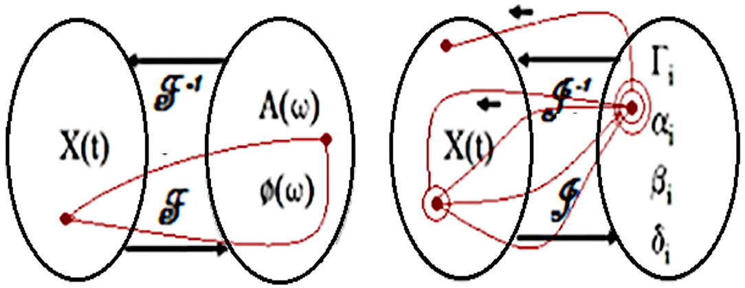
Figure 7. Left: Correspondence between the signal and Fourier transform vector spaces. Right: Correspondence between the signal and Tailored to the Problem Specificity (TPS) transform vector spaces.

Upgrading Current Tailored to the Problem Specificity Methodology

In a previous study, an eight steps methodology was defined to solve TPS MT [3]. Steps considered are:

• Identify basic components and select a realistic model.

• Collect the data.

• Use “adequate coding” to improve processes.

• Buildup the data training set (TS).

• Choose a supervised algorithm.

• While in previous study, backpropagation was selected to perform JT, in current study, ELM is suggested to be used to calculate JT and other TPS transforms.

• Calculate error.

• Perform the TPS transform using a training machine learning algorithm

• Process recognition and testing phases with a trained computer intelligence algorithm.

Discussion

As previously pointed out, if TPS is possible, basis could express causality better than linear transforms and “fundamental and technical analysis” would be congruent between each other. Yet it remains the following steps:

• Formalize a restrained vector space (for the mathematical descriptions of the proposed TPS transforms).

• Restrict the space of solutions of the system equation.

• Introduce ELM with a new topological construction.

• Identify TPS parameters.

• Improve the formalization of the expected results.

This article can be considered as a trial to use ELM instead of backpropagation learning rule in solving TPS, such as Jewett transform, as well as an informal venture into the definition of Glover, Friston, and Latham transforms and a first attempt to link Dynalet transform with TPS transforms.

Perspectives and Conclusion

A recent improvement of TPS MT approach is the functional principal component analysis (FPCA), a tool of dimension reduction with high correlations in functional data analysis [33, 34], which is used in epidemiologic problems as those related to coronavirus disease 2019 (COVID-19) outbreak dynamics, as given in Figure 8 [35–45].

FIGURE 8

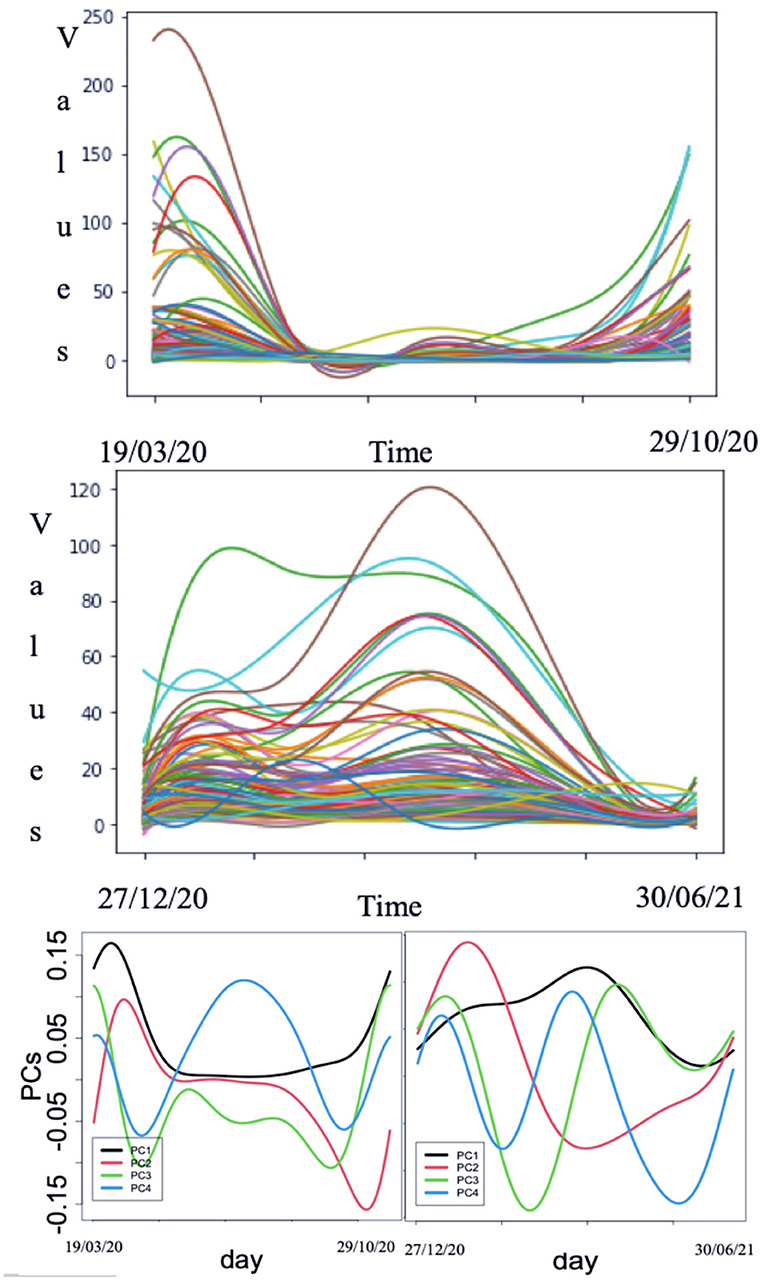
Figure 8. Smoothed curves for coronavirus disease 2019 (COVID-19) hospitalization cases in all the departments in France before (top) and after (middle) vaccination. Bottom: Functional principal components (PCs) for the above hospitalization case curves (after [35]).

Let {x_i(t)}_{i = 1,m} be a given set of functions and let denote α = (α₁, …, α_m) a weight vector, FPCA is calculated such as it finds, in the set of the C₁ functions on the time interval of observation, the first principal component weight function α₁(t), for which the first principal component score is given by:

$\begin{array}{ll}{f}_{i1}={\displaystyle \int }{\alpha }_1\left(t\right)x_i\left(t\right)dt,& (33)\end{array}$

while maximizing ${\sum }_{i=1,m}{f}_{i1}^2$ is subjected to:

$\begin{array}{ll}{\displaystyle \int }{\alpha }_1^2\left(t\right)dt=\Vert {\alpha }_1{\Vert }^2=1.& (34)\end{array}$

Next, the weight function α₂(t) is calculated and the second principal component score maximizes $\sum _{i=1,m}{f}_{i2}^2$, and is subjected to the constraints ${\Vert {\alpha }_2\Vert }^2=1$ and:

$\begin{array}{ll}{\displaystyle \int }{\alpha }_2\left(t\right){\alpha }_1\left(t\right)dt=0.& (35)\end{array}$

Then, the process is repeated for many iterations. In our analysis, we used a tool called pca.fd for the principal component analysis. As given in Figure 8, the 4 PCs values plots throughout the days considered for all the m (m = 101) French departments providing functional data being before vaccination started and during vaccination. Table 1 gives the weight of each PC for the curves of hospitalization before and after vaccination has started.

TABLE 1

Table 1. Principal component analysis (PCA) variance proportion for 4 PCs.

This last example shows that the TPS approach is still here relevant and can be considered as a valid concrete alternative to realistically approach the modeling of temporal data in epidemiological [46–51] or physiological [24, 52] examples.

To conclude, even with the recent techniques of the functional principal component analysis (FCPA), the TPS MT approach is relevant, in the sense that it makes it possible to consider the experimental signal as a linear combination of functions that are the weighted sum (not necessarily orthogonal) of the main empirical variables of the system source of the recorded signal, in a decreasing order of importance, which allows the interpretation of the respective role of the empirical variables in the generation of this signal.

Data Availability Statement

The original contributions presented in the study are included in the article/supplementary material, further inquiries can be directed to the corresponding author.

Ethics Statement

Ethical review and approval was not required for the study on human participants in accordance with the local legislation and institutional requirements. The patients/participants provided their written informed consent to participate in this study.

Author Contributions

JD and AG: conceptualization, methodology, validation, formal analysis, resources, writing—original draft preparation, supervision, and project administration. KO and CT: software. AG, JD, RS, SC, PR, AA, GT, MS, HZ, CT, and KO: investigation. AA, GT, MS, HZ, CT, and KO: data curation. JD and KO: writing—review and editing. KO, CT, and AG: visualization. All authors have read and agreed to the final version of the manuscript.

Funding

The authors acknowledge to support Chilean Grants DIUV 44/11 from U. de Valparaiso, Fondecyt MEC 80110027, and FONDEF IT13I20060 from Conicyt.

Conflict of Interest

The authors declare that the research was conducted in the absence of any commercial or financial relationships that could be construed as a potential conflict of interest.

Publisher's Note

All claims expressed in this article are solely those of the authors and do not necessarily represent those of their affiliated organizations, or those of the publisher, the editors and the reviewers. Any product that may be evaluated in this article, or claim that may be made by its manufacturer, is not guaranteed or endorsed by the publisher.

Acknowledgments

We want to honor Jean Baptiste Joseph Fourier in the bicentennial of the end of his master pieces, written at Grenoble between 1808 and 1822. Joseph Fourier was a living example of the idea of a tailored to problem model. Taking up ideas from the Bourguignon Buffon, Joseph Fourier modeled fluid dynamics (work taken up by his Dijon polytechnic students Darcy and Navier) and cooling of the earth, making it possible to calculate its age. This last study has been taken up in an exciting scientific debate by Lord Kelvin and Charles Darwin, after the latter's visit to Chile, namely, to the Campana massif. Quoting studies by Fourier and Claude Gay (pioneer, with Louis Lliboutry, of the geology of Chile), Darwin explained with geologist's arguments that earth was several hundred million years old, while Kelvin calculated a few dozen, using a model mathematically rigorous but not tailored to the problem. Both were wrong, but Darwin was closer to the truth.

References

1. Kreider DL, Kuller RG, Öestberg DR, Perkins FW. An Introduction to Linear Analysis. Reading PA: Addison-Wesley (1966).

2. Demongeot J, Glade N, Forest L. Liénard systems and potential-Hamiltonian decomposition. C. R. Mathématique. (2007) 344:121–6. doi: 10.1016/j.crma.2006.10.016

PubMed Abstract | CrossRef Full Text | Google Scholar

3. Glaría A, Taramasco C, Demongeot J. Methodological Proposal to estimate a Tailored to the Problem Specificity Mathematical Transformation. In: IEEE AINA'10. Piscataway: IEEE Proceedings (2010), p. 775–81.

Google Scholar

4. Huan GB, Zhu QY, Siew CK. Extreme learning machine: THEORY and applications. Neurocomputing. (2006) 70:489–501. doi: 10.1016/j.neucom.2005.12.126

CrossRef Full Text | Google Scholar

5. Jewett DL, Willinston JS. Auditory-evoked far fields averaged from the scalp of humans. Brain. (1971) 4:681–96. doi: 10.1093/brain/94.4.681

PubMed Abstract | CrossRef Full Text | Google Scholar

6. Glaría A, Roncagliolo M, Montero H, Castro A. Non-orthogonal components for the analysis of auditory Brainstem Average Evoked Responses (BSR): towards a physiological basis. In: IV^th Medit. Conf. Med. Biol. Eng. Sevilla: Mecombe (1986). p. 549–52.

7. Baruch MC, Warburton DER, Bredin SSD, Cote A, Gerdt DW, Adkins CM. Pulse Decomposition Analysis of the digital arterial pulse during hemorrhage simulation. Nonlinear Biomed Phys. (2011) 5:1–15. doi: 10.1186/1753-4631-5-1

PubMed Abstract | CrossRef Full Text | Google Scholar

8. Latham RD, Westerhof N, Sipkema P, Rubal BJ, Reuderink P, Murgo JP. Regional wave travel and reflections along the human aorta: a study with six simultaneous micromanometric pressures. Circulation. (1985) 72:1257–69. doi: 10.1161/01.CIR.72.6.1257

PubMed Abstract | CrossRef Full Text | Google Scholar

9. Buxton R, Wong EC, Frank LR. Dynamics of blood flow and oxygenation changes during brain activation: the Balloon Model. Magn Res Med. (1998) 39:855–64. doi: 10.1002/mrm.1910390602

PubMed Abstract | CrossRef Full Text | Google Scholar

10. Glover G. Deconvolution of impulse response in event-related bold fMRI. Neuroimage. (1999) 9:416–29. doi: 10.1006/nimg.1998.0419

PubMed Abstract | CrossRef Full Text | Google Scholar

11. Friston K, Joseph O, Ress G, Turner R. Non-linear event-related response in fMRI. Magn Res Med. (1997) 38:41–52. doi: 10.1002/mrm.1910390109

PubMed Abstract | CrossRef Full Text | Google Scholar

12. Demongeot J, Glade N, Forest L. Liénard systems and Potential-Hamiltonian decomposition. II. Algorithm. C R Math. (2007) 344:191–4. doi: 10.1016/j.crma.2006.10.013

PubMed Abstract | CrossRef Full Text | Google Scholar

13. Demongeot J, Hamie A, Glaría A, Taramasco C. Dynalets: a new representation of periodic biological signals and spectral data. In: IEEE AINA'13. Piscataway: IEEE Proceedings (2013), p. 1525–32. doi: 10.1109/WAINA.2013.174

CrossRef Full Text | Google Scholar

14. van der Pol B. On relaxation oscillations. In: The London, Edinburgh, and Dublin Philosophical Magazine and Journal of Science, Vol.2. London: Taylor and Francis (1926). p. 978–92. doi: 10.1080/14786442608564127

CrossRef Full Text | Google Scholar

15. van der Pol B, van der Mark J. Le battement du cœur considéré comme oscillation de relaxation et un modèle électrique du cœur. Onde Elect. (1928) 7:365–92.

16. McDonald KT, Maloney TJ. Leaky Capacitors. Princeton: Princeton University. (2001).

17. Glaría A, Arancibia C. Neural Network techniques for a physiologically rooted Analysis of Auditory Brainstem Average Evoked Responses. In: IEEE ICNN'96. Piscataway: IEEE Proceedings (1996), p. 800–3.

18. Finapres Medical Systems (2015). Available online at: http://www.finapres.com/Products/Finapres-NOVA (accessed January 6, 2022).

19. Tapia G, Glaría A. Red Neuronal Artificial para detectar esfuerzo físico desde Planos de Fase de Onda de Pulso. Rev Ing. Bioméd. (2015) 9:21–34.

Google Scholar

20. Salinas M. Hacia una TPS WK Para la Estimación de la Presión Arterial. In: Congreso Anual de Ingeniería Biomédica 2016. Concepción: Universidad de Concepción (2016).

21. Frank O. Die grundform des arterielen Pulses Erste Abhandlung: Mathematische Analyse. Z Biol. (1899) 37:483–526.

Google Scholar

22. Guairini M. Estimation of cardiac function from computer analysis of the arterial pressure waveform. IEEE Trans Biomed Eng. (1998) 45:1420–28. doi: 10.1109/10.730436

PubMed Abstract | CrossRef Full Text | Google Scholar

23. Zepeda H. Aplicación de la Transformada Matemática TPS en la estimación de HRF para la detección de Activación Neuronal en imágenes f-MRI. (Master Thesis Ingeniero Civil Biomédico). Valparaiso: University Valparaíso. (2016).

24. Demongeot J, Khlaifi H, Istrate D, Mégret L, Taramasco C, Thomas R. From conservative to dissipative non-linear differential systems. An application to the cardio-respiratory regulation. Discrete Contin Dyn Syst. (2020) 13:2121–34. doi: 10.3934/dcdss.2020181

CrossRef Full Text | Google Scholar

25. Hodge W. The Theory and Applications of Harmonic Integrals. Cambridge: Cambridge University Press (1941).

Google Scholar

26. Demongeot J, Hansen O, Hamie A. Dynalets: a new tool for biological signal processing. In: Medicon'13. IFBME Proc. 41. New York, NY: Springer (2014), p. 1250–3.

Google Scholar

27. Demongeot J, Hansen O, Hamie A, Rachdi M. Dynalets: a new tool for biological signal processing. In: ICPS'13. New York, NY: Springer (2015), p. 141–50. doi: 10.1007/978-3-319-22476-3_9

CrossRef Full Text | Google Scholar

28. https://www.sciences.univ-nantes.fr/sites/genevieve_tulloue/Meca/Oscillateurs/vdp_phase.php (accessed February 22, 2022).

29. Glaría A, Zepeda H, Chabert S, Hidalgo M, Demongeot J, Taramasco C. Complex adaptive systems with inference learning emergent property to estimate Tailored to the Problem Specificity Mathematical Transforms: three study cases. In: ECCS'13. Barcelona: Complex Syst. Soc. (2013), p. 127–9.

Google Scholar

30. Fourier JBJ. Digression sur la manière d'exprimer les fonctions arbitraires par des séries de quantités périodiques. In: Théorie mathématique de la chaleur. Chapitre VII. Paris: Firmin Didot Père et Fils (1822).

31. Lejeune-Dirichlet JPG. Sur la convergence des séries trigonométriques qui servent à représenter une fonction arbitraire entre des limites données. J Reine Angew Math. (1829) 4:157–69. doi: 10.1515/crll.1829.4.157

CrossRef Full Text

32. Dahlgren F. Partial continuous functions and admissible domain representations. J Log Comput. (2007) 17:1063–81. doi: 10.1093/logcom/exm034

CrossRef Full Text | Google Scholar

33. Ramsay JO, Silverman BW. Applied Functional Data Analysis: Methods and Case Studies. New York, NY: Springer. (2002). doi: 10.1007/b98886

CrossRef Full Text | Google Scholar

34. Srivastava A, Klassen EP. Functional and shape data analysis. In: Srivastava A, Klassen EP, editors. Functional Data and Elastic Registration. Berlin: Springer (2016). p. 73–122. doi: 10.1007/978-1-4939-4020-2_4

CrossRef Full Text | Google Scholar

35. Griette Q, Demongeot J, Magal P. A robust phenomenological approach to investigate COVID-19 data for France. Math Appl Sci Eng. (2021) 2:149–60. doi: 10.1101/2021.02.10.21251500

CrossRef Full Text | Google Scholar

36. Demongeot J, Flet-Berliac Y, Seligmann H. Temperature decreases spread parameters of the new covid-19 cases dynamics. Biology. (2020) 9:94. doi: 10.3390/biology9050094

PubMed Abstract | CrossRef Full Text | Google Scholar

37. Demongeot J, Seligmann H. Covid-19 and miRNA-like inhibition power. Med Hypotheses. (2020) 144C:110245. doi: 10.1016/j.mehy.2020.110245

PubMed Abstract | CrossRef Full Text | Google Scholar

38. Demongeot J, Griette Q, Magal P. Computations of the transmission rates in SI epidemic model applied to COVID-19 data in mainland China. R Soc Open Sci. (2020) 7:201878. doi: 10.1098/rsos.201878

PubMed Abstract | CrossRef Full Text | Google Scholar

39. Soubeyrand S, Demongeot J, Roques L. Towards unified and real-time analyses of outbreaks at country-level during pandemics. One Health. (2020) 11:100187. doi: 10.1016/j.onehlt.2020.100187

PubMed Abstract | CrossRef Full Text | Google Scholar

40. Demongeot J, Oshinubi K, Rachdi M, Seligmann H, Thuderoz F, Waku J. Estimation of daily reproduction rates in COVID-19 outbreak. Computation. (2021) 9:109. doi: 10.3390/computation9100109

CrossRef Full Text | Google Scholar

41. Gaudart J, Landier J, Huiart L, Legendre E, Lehot L, Bendiane MK, et al. Factors associated with spatial heterogeneity of Covid-19 in France: a nationwide ecological study. Lancet Public Health. (2021) 6:e222–31. doi: 10.1016/S2468-2667(21)00006-2

PubMed Abstract | CrossRef Full Text | Google Scholar

42. Oshinubi K, Ibrahim F, Rachdi M, Demongeot J. Functional data analysis: application to daily observation of COVID-19 prevalence in France. AIMS Math. (2022) 7:5347–85. doi: 10.3934/math.2022298

CrossRef Full Text | Google Scholar

43. Griette Q, Demongeot J, Magal P. What can we learn from COVID-19 data by using epidemic models with unidentified infectious cases? Math Biosci Eng. (2022) 19:537–94. doi: 10.3934/mbe.2022025

PubMed Abstract | CrossRef Full Text | Google Scholar

44. Oshinubi K, Rachdi M, Demongeot J. Modelling of COVID-19 pandemic vis-à-vis some socio-economic factors. Front Appl Math Stats. (2022) 7:786983. doi: 10.3389/fams.2021.786983

CrossRef Full Text | Google Scholar

45. Oshinubi K, Rachdi M, Demongeot J. Approach to COVID-19 time series data using deep learning and spectral analysis methods. AIMS Bioeng. (2022) 8:9–21. doi: 10.3934/bioeng.2022001

CrossRef Full Text | Google Scholar

46. Glade N, Forest L, Demongeot J. Liénard systems and Potential-Hamiltonian decomposition. III Applications. C R Math. (2007) 344:253–8. doi: 10.1016/j.crma.2006.11.014

PubMed Abstract | CrossRef Full Text | Google Scholar

47. Demongeot J, Glade N, Forest L. Liénard systems and Potential-Hamiltonian decomposition. IV Applications in Biology. C R Biol. (2007) 330:97–106. doi: 10.1016/j.crvi.2006.12.001

PubMed Abstract | CrossRef Full Text | Google Scholar

48. Contreras G, Glaría A. Codifying temporal characteristics of Jewett Transform. J Phys. (2007) 90:012075. doi: 10.1088/1742-6596/90/1/012075

CrossRef Full Text

49. Demongeot J, Hamie A, Hansen O, Franco C, Sutton B, Cohen EP. Dynalets: a new method of modelling and compressing biological signals. Applications to physiological and molecular signal. C R Biol. (2014) 337:609–24. doi: 10.1016/j.crvi.2014.08.005

PubMed Abstract | CrossRef Full Text | Google Scholar

50. Fourier JBJ. Mémoire sur la propagation de la chaleur dans les corps solides. Nouv Bull Sci Soc Philom Paris. (1808) 1:112–6. doi: 10.1017/CBO9781139568159.003

CrossRef Full Text

51. Hornik K, Stinchcome M, White H. Multilayer Feedforward networks are Universal approximators. Neural Netw. (1989) 2:359–66. doi: 10.1016/0893-6080(89)90020-8

CrossRef Full Text | Google Scholar

52. Pham Dinh T, Demongeot J, Baconnier P, Benchetrit G. Simulation of a biological oscillator: the respiratory rhythm. J Theor Biol. (1983) 103:113–32. doi: 10.1016/0022-5193(83)90202-3

PubMed Abstract | CrossRef Full Text | Google Scholar