Estimation of Some Epidemiological Parameters With the COVID-19 Data of Mayotte

1. Introduction

Following the emergence of the COVID-19 and its spread outside of China, all countries are experiencing the pandemic. The COVID-19 virus has caused great disruption to human health, social life, development, and economics. In response, several countries have implemented several interventions including nonpharmaceutical, vaccination, case isolation of symptomatic individuals and their contacts, restriction and social distancing in schools, at work, and universities, banning of mass gatherings and some public events, and local and national lockdowns of populations. Also in response to the rising numbers of cases and deaths, and to maintain the capacity of health systems to treat as many severe cases as possible, France like European countries and other continents has implemented some process measures to control the epidemic, (refer to [1–4]). In the French overseas department, especially in Mayotte, there is a high population density and certain local issues such as access to water, housing, hindering distance measures, and barrier gestures. The epidemic data in Mayotte started on 13 March 2020 when the first reported case traveled from metropolitan France (3 days ago with two other family members, which in turn were confirmed positive a few days later). Some other imported cases were confirmed later and led to the actual state of the spread of the virus in Mayotte. Many mathematical models of the COVID-19 coronavirus epidemic have been developed, and some of these are listed in the following articles [5–12, 42]. Based on the development of epidemiological characteristics of COVID-19 infection, a model of type SEIARS can be appropriate to study the dynamics of this disease. To understand trends in the development of the epidemic curve, it is important to know the serial interval distribution of the COVID-19 virus estimate and hence the generation time to be able to give some estimation of the epidemiological parameters like the time- varying reproduction number and observed transmission rates, among others. This article aims to study first the statistical methods to fit the probability distribution function which underlines the serial interval distribution of the COVID-19 virus on a given set of data collected on the viral shedding in patients with laboratory-confirmed COVID-19 (refer to [13, 14]) to obtain a best-fit model of the serial interval distribution. Based on this estimation, we estimate the time- varying reproduction number and the transmission rates observed on the island of Mayotte from March 2020 to January 2022. The paper is organized as follows. We present the material and methods sections, the data, and the statistical tools together with the mathematical learning model and tools. In the result section, we give the estimation of the serial interval distribution by several methods and the best-fit model with a mixture model. We derive an estimation of the effective reproduction number along the time. We fit the transmission rates parameters range values obtain through the mathematical learning model together with a sensitivity analysis of some parameters like the asymptotic ratio and infectious period ratio. The results are presented together with along with a discussion. We also present some regression and forecasting models for the hospitalized, intensive care, and death cases over a given period. We end with a conclusion and the limit of this study and some theoretical perspectives as forthcoming work.

2. Material

This study is concerned with a statistical analysis of some important parameters of the COVID-19 epidemic curve in Mayotte.

2.1. Observed COVID-19 Infected Cases in Mayotte

Many efforts have been made by the French Regional Health Agencies in Mayotte to collect the data. The present study is based on a reported dataset of confirmed cases of COVID-19 from 13 March 2020 to 11 January 2022. The reported temporal daily cases and total confirmed cases are illustrated in Figure 1. We also consider a subset of the database containing the daily observed cases of confirmed hospitalization, intensive care, and death cases from 13 March 2020 to 26 February 2021 in Figure 1.

FIGURE 1

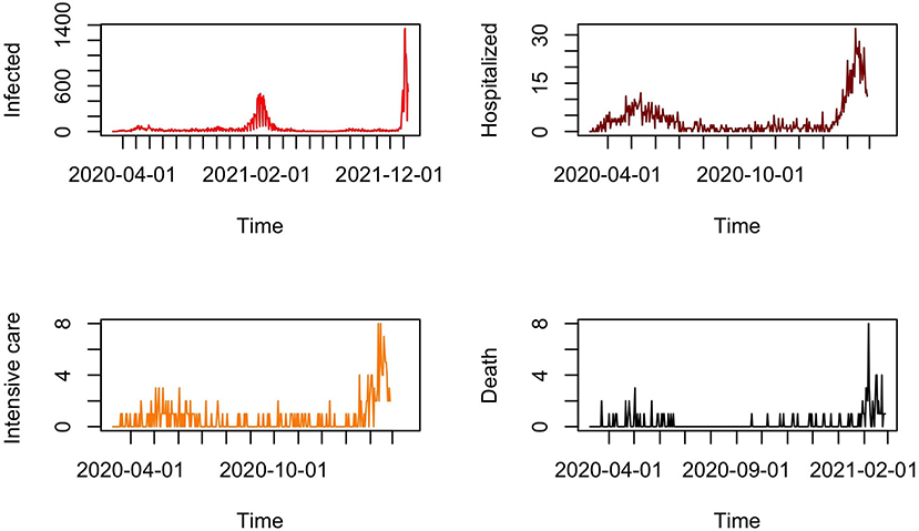
Figure 1. Reported daily infected cases from 13 March 2020 to 11 January 2022 and reported daily cases of hospitalization, intensive care, and death cases from 13 March 2021 to 26 February 2021 in Mayotte.

2.2. COVID-19 Infectiousness Profiles From Transmission Pairs

Some major studies have been made on the determination of generation times through serial interval distributions and incubation time from real data, refer to for instance [13, 14]. In this section, we will focus on the data collected by He et al. [13] where the authors report temporal patterns of viral shedding in 94 patients with laboratory-confirmed COVID-19 and modeled COVID-19 infectiousness profiles from a separate sample of 77 infector-infectee transmission pairs. The variation between individuals (infector/infectee) and the transmission process is summarized, respectively by the distribution of incubation period and serial intervals. Figure 2 (picture above) contains the number of infected cases (in red), the lower limit of infectors (in black), and the upper limit of infectors (in green).

FIGURE 2

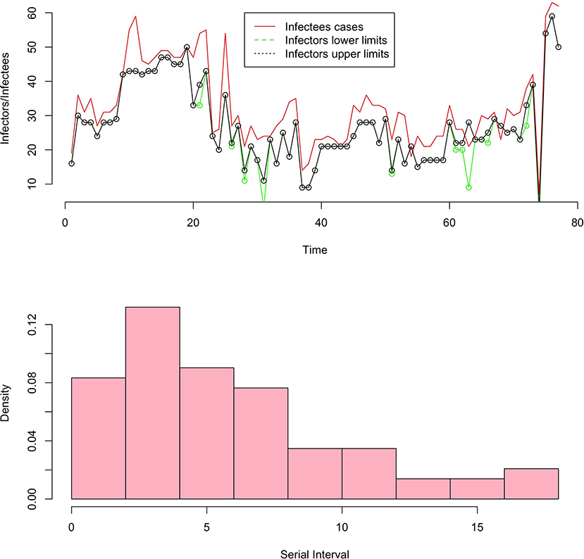
Figure 2. Evolution of the infector and infectee pairs and histogram of the serial interval.

The variation between individuals and chains of transmission is summarized, respectively by the distribution of incubation periods and the distribution of serial intervals (refer to definition below). For simplicity, we consider non-negative serial interval values which represent 93% of the data. Figure 2 shows the histogram (picture below) of the serial interval from the underline database.

3. Methods

First let us recall some definitions concerning the infectivity process. Consider an infector i and infectee j. The generation time interval ${{G}}_{i,j}$ is the time interval from the infection of i to infection of j. It is the time lag between infection in a primary case and a secondary case; and should be obtained from the time lag between all infectee/infector pairs [15]. In this way, it describes infectiousness with respect to the point of infection. As it cannot be observed directly, it is often substituted with the serial interval distribution ${{S}}_{i,j}$ which is the time interval between symptom onset of the infector i and symptom onset of the infectee j. They can be captured by the following equations:

$\begin{array}{l}{{G}}_{i,j}={{S}}_{i,j}+{{E}}_i-{{E}}_j\end{array}$

or

$\begin{array}{l}{{G}}_{i,j}={{P}}_{i,j}-P_{j,i}+{{S}}_{j,i}.\end{array}$

where ${E}$ is the time interval between symptom onset and the infection (incubation period) and ${{P}}_{i,j}$ is the time interval from the symptom onset of i to infection of j. We refer the reader to Lehtinen et al. [16] and Svensson [15] for further details. The serial interval that can be computed as follow (refer to [13]):

$\begin{array}{l}serial\text{\_}interval=y-(\frac{x.ub+x.lb}{2})\end{array}$

with

• x.lb: Lower limit dates of onset of symptoms of infectors.

• x.ub: Upper limit dates of onset of symptoms of infectors.

• y: Dates of onset of symptoms of the infectee.

There are many methods for generating estimates of parameters for standard probability distributions such as the method of moments and the maximum likelihood estimation. The use of other methods was generally confined to analytical work on mixture densities. Rapid analysis of the above histogram seems to show that the serial interval can be fit by a set of exponential- family distributions (e.g., «Gamma », «Lognormal », «Weibull », and «Exponential »distributions) or a mixture of them. The method of moments consists in estimating the parameters of the distributions from the theoretical finite moments with their empirical estimates. As concerned the Weibull distribution, we estimate the scale and shape parameters from the analytical expression of the mean, median, and the variance of the above serial interval data.

3.1. Estimation by the Maximum Likelihood Method

The maximum likelihood estimation (refer to [17] is a statistical method used to estimate the parameters of the probability law of a given observation x = (x₁, .., x_n) with probability densities f(x_i, θ) by determining the values of the parameters maximizing the log-likelihood function given by:

$L(\theta )=log({\displaystyle \prod _{i=1}^n}f(x_i,\theta ))={\displaystyle \sum _{i=1}^n}log(f(x_i,\theta ))$

where θ is the (vector) parameter to be estimated. The likelihood function then represents the joint density of the individual observations x_i for any given level of the distribution parameters. The maximum likelihood estimate is the distribution parameter values, which maximize the likelihood function since these same values of the estimators also maximize the log-likelihood function.

3.2. Estimation by a Mixture Method

We present a mixture estimation which is a flexible tool (see [18, 19]) to model a known smooth probability density function as a weighted sum of parametric density functions f_j(x, θ_j) in a possibly multivariate independent observations x = (x₁, .., x_n) drawn from k several densities:

$\begin{array}{l}f(x)={\displaystyle \sum _{j=1}^k}{p}_j{f}_j(x,{\theta }_j)\end{array}$

where k represents the number of classes or groups of the mixing, p_j>0 is the relative proportion of observations from each class j such that $\sum _{j=1}^n{p}_j=1.$ The mixture density will allow finding the parameter Θ = (p_j, θ_j) of the model where θ_j is the (vector) parameter from class j. The log-likelihood of the mixing density is defined by:

$\begin{array}{l}L(\Theta )=log({\displaystyle \prod _{i=1}^n}f(x_i,\Theta ))={\displaystyle \sum _{i=1}^n}log({\displaystyle \sum _{j=1}^k}{p}_j{f}_j(x_j,{\theta }_j)).\end{array}$

The maximum likelihood estimates are:

$\begin{array}{l}max{\displaystyle \sum _{i=1}^n}\left\{log({\displaystyle \sum _{j=1}^{k-1}}(p_j{f}_j(x_i,{\theta }_j))+(1-{\displaystyle \sum _{j=1}^{k-1}}{p}_j)f_k(x_i,{\theta }_k))\right\}\end{array}$

subject to

$\begin{array}{l}{\displaystyle \sum _{j=1}^{k-1}}{p}_j\le 1.\end{array}$

For k>1, the sum of the term appearing inside a logarithm makes this optimization quite difficult. Solution of this non-linear optimization problem has long been a difficult task for applied researchers. There are, of course, many general iterative procedures that are suitable for finding an approximate solution to the likelihood equations.

3.3. Non Parametric Estimation of the Time Varying Reproduction Number

Understanding the development of an epidemic is important as well as the basic reproduction number ℝ₀ at the start of an epidemic and the time varying reproduction numbers. It is historically defined as the average number of new cases of infection generated by an individual during a period of infectivity (refer to [20]). There are several methods for computing this parameter, e.g., the next-generation matrix method. Let us mention here a non-parametric approach following Wallinga and Lipsitch [21]. Let η be the probability that an individual will remain infectious over a unit of time after being infected (i.e., age of infection) and β the transmission rate at age of infection a. Then τ(a) = η(a)β(a) is the transmissibility of an infectious individual at the age of infection a, assuming that the entire population is susceptible. Hence,

$\begin{array}{l}{R}_0={\displaystyle {\int }_{a=0}^{\infty }}\tau (a)\text{d}a.\end{array}$

We can normalize τ(a) to be a probability density function:

$\begin{array}{l}w(a)=\frac{\tau (a)}{{\displaystyle {\int }_{a=0}^{\infty }}\tau (s)\text{d}s}\\ =\frac{\tau (a)}{R_0}.\end{array}$

so that

$\begin{array}{l}\tau (a)=R_{0}w(a).\end{array}$

Let Γ(t) be the number of new infections during the time interval ]t; t+dt[ and s(t) the proportion of susceptibles in the population. Note that the new infections at time t are the sum of all infections caused by infectious individuals infected at a unit of time (i.e., at time t = a) if they remain infectious at time t (with an infectious age a). In other words

$\begin{array}{l}\Gamma (t)={\displaystyle {\int }_0^{\infty }}\Gamma (t-a)\tau (a)s(t)\text{d}a=s(t){\displaystyle {\int }_0^{\infty }}\Gamma (t-a)\tau (a)\text{d}a\\ =s(t){\displaystyle {\int }_0^{\infty }}\Gamma (t-a)w(a)R_0\text{d}a.\end{array}$

For t≠0, we have a non parametric formula of the time varying reproduction number

$\begin{array}{l}{R}_0(t)=R_0*s(t)=\frac{\Gamma (t)}{{\displaystyle {\int }_0^{\infty }}\Gamma (t-a)w(a)\text{da}}.\end{array}$

For practical calculation, this formula offers a discrete version as follows

$\begin{array}{ll}{R}_0(t)=\frac{\Gamma (t)}{{\displaystyle {\sum }_{\tau \le t}}w(\tau )\Gamma (t-\tau )},& (1)\end{array}$

implemented in the package R0, Obadia et al. [22] and Boelle et al. [23] and package EpiEstim, [24, 25]. In this study, we will compare our results on the reproduction numbers with the R₀ package. For more on the calculation of the R₀, we refer to Batista [26]. Other improved estimation methods also exist in the literature, refer to Demongeot et al. [27] and Waku et al. [28], and references therein.

3.4. Regression and Forecasting Models

A regression method (refer to [29]) is a predictive statistical approach for modeling the relationship between a dependent variable say Y with a given set of observed variables say X = (X₁, X₂, …, X_n) under the form Y = f(X, η)+ω, where η is an unknown (vector) parameter and ω representing an additive error that may stand for white noise. The prediction models provide the insights that result in tangible outcomes.

The predictive statistical approach for disease research work found in the literature deals with ARIMA models [30, 31], polynomial regression and hierarchical polynomial regression models [32–34]. Recall that a process Y_t is said to be ARIMA(p, d, q) if

$\begin{array}{l}{Y}_t=\alpha +{\displaystyle \sum _{i=1}^p}{\varphi }_i{Y}_{t-i}+{\displaystyle \sum _{j=1}^q}{\theta }_j{\omega }_{t-j}+{\omega }_t,\end{array}$

where Y_t−1, Y_t−2, ..., Y_t−p are the lags (past values); ϕ₁, ϕ₂, ..., ϕ_p are lag coefficients that are estimated by the model; ω_t−1, ω_t−2, ..., ω_t−q are error terms of the model for the respective lags; θ₁, θ₂, ..., θ_q their coefficients, and

$\begin{array}{l}\alpha =(1-{\displaystyle \sum _{i=1}^p}{\varphi }_i)\mu \end{array}$

with μ the mean of the process. When analyzing a model, it is important to measure its performance in order to draw the best conclusion and interpretation of the data. We will use the coefficient of determination or R² as a metric given by

$\begin{array}{l}{R}^2=1-\frac{S{S}_{res}}{S{S}_{tot}},\end{array}$

where for n values marked y₁, ..., y_n, each associated with a fitted value ŷ₁, ..., ŷ_n, the sum of squares of residuals $S{S}_{res}=\sum _i^n(y_i-{ŷ}_i)$, and the total sum of squares $S{S}_{tot}=\sum _{i=1}^n(y_i-ȳ)$.

3.5. The Mathematical Learning Model

We propose a simple model that generalizes the SEIR model commonly used for virus disease modeling. The total population is partitioned into the following compartments: Susceptible S, Exposed E, Infected but not yet infectious, in a latent homogeneous period λ⁻¹; symptomatic Infected I_s with infectious period ${\gamma }_1^{-1}$ and asymptomatic Infected I_a in an infectious period ${\gamma }_2^{-1}$; Recovered R cases, and disease Dead cases D. We assume that every Exposed subject that enters I_s cohort later develops symptoms with probability 1−q and those who do not enter the I_a cohort with probability q. This assumption comes from real information in Mayotte and can be seen also in some studies, refer to Mizumoto et al. [35, 36]. We assume that a protected fraction ω of recovered individuals move to S (loss of immunity and re-infection). Given initial conditions S(0)>0, E(0)>0, I_s(0)>0, I_a(0)>0, R(0)>0, and D(0)≥0, the differential equations that govern the trajectories of our model are formulated as follow

$\{\begin{array}{l}dS(t)=-\beta S\frac{(I_s+I_a)}{N}dt+\omega Rdt\\ dE(t)=\beta S\frac{(I_s+I_a)}{N}dt-\lambda Edt\\ d{I}_s(t)=(1-q)\lambda Edt-({\gamma }_1+\alpha )I_{s}dt\\ d{I}_a(t)=q\lambda Edt-{\gamma }_2{I}_{a}dt\\ dR(t)={\gamma }_1{I}_{s}dt+{\gamma }_2{I}_{a}dt-\omega Rdt\\ dD(t)=\alpha I_{s}dt\end{array}$

where N = S+E+I_s+I_a+R+D is the fixed total population. With the initial conditions, the above system is well posed, with all variables remaining non-negative and N positive constant.

The epidemic equilibrium X₀ of the system is obtained by setting all the derivatives to zero with I_s = I_a = 0, which yields to X₀ = (N, 0, 0, 0, 0). To obtain the basic reproduction number, we use the next generation matrix (Dieckmann) by writing the Jacobian matrix of the flows of individuals between the different compartments at equilibrium:

$F=\left(\begin{array}{ccc}0& \beta & \beta \\ 0& 0& 0\\ 0& 0& 0\end{array}\right)$

$V=\left(\begin{array}{ccc}\lambda +\mu & 0& 0\\ -(1-q)\lambda & {\gamma }_1+\alpha & 0\\ -q\lambda & 0& {\gamma }_2\\ \end{array}\right)$

The Jacobian matrix FV⁻¹ has two zero and one positive eigenvalues so that

$\begin{array}{l}{R}_0=\frac{q\beta }{{\gamma }_2}+\frac{(1-q)\beta }{{\gamma }_1+\alpha }.\end{array}$

Considering the negligible death rate, we have

$\begin{array}{l}{R}_0~\beta (\frac{q}{{\gamma }_2}+\frac{1-q}{{\gamma }_1}).\end{array}$

Thus

$\begin{array}{ll}\beta ~\frac{R_0{\gamma }_1}{r+1-q},& (2)\end{array}$

where ratio $r:=\frac{{\gamma }_1}{{\gamma }_2}.$ We assume in this article that, due to the isolation the symptomatic individual reduces their infectiousness so we shall consider values of r less than one.

4. Results and Discussion

The purpose of this section is to present the results not only on the parameter estimation of the serial interval distribution, and the reproduction numbers but also estimates of the transmission rates based on the above simple model.

4.1. Estimation of the Serial Interval

The basic method of moments (Figure 3A) and maximum likelihood estimation (Figure 3B) are summarized in Figure 3 for a set of classical distributions.

FIGURE 3

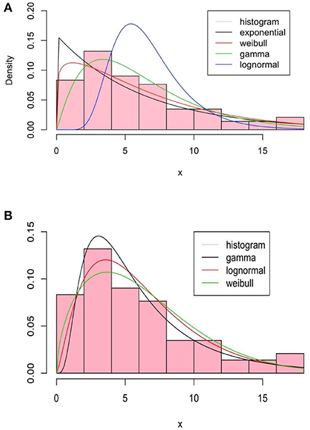
Figure 3. Summary of the method of moments, (A), and by the maximum likelihood estimation (MLE), (B), of fitted distributions.

As we can see in the method of moments, the «Gamma »distribution seems to fit better than others. Note that the method of moments does not give a good fit since it does not use any optimization techniques such as the Maximum Likelihood Estimation (MLE) method. The fit with the exponential distribution is not good and in the sequel, we will focus on «Gamma », «Lognormal », and «Weibull »distributions. The Kolmogorov-Smirnov test result for them is given also in Table 1 for the method of moments.

TABLE 1

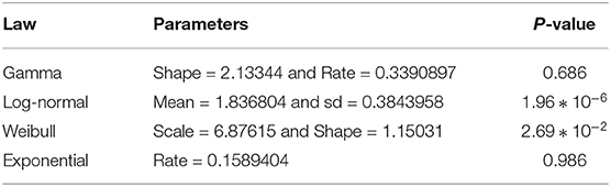
Table 1. Explicit fitted parameters by the method of moments and Kolmogorov-Smirnov test.

The maximum likelihood estimate is done using the R software function nlm, refer to Obadia et al. [22]. In Figure 3B, we represent several fitted densities estimated by this method.

We can see that, compared to the method of moments, the maximum likelihood improves in some way the estimation, refer to Table 2 for the Kolmogorov test. Akaike's Information Criterion (AIC) and the Bayesian Information Criterion (BIC) are written as follows:

$\begin{array}{l}\text{AIC}=2k-2log(L)\text{BIC}=-2log(L)+klog(N),\end{array}$

where k is the number of parameters to estimate, L is the maximum of the likelihood function of the model, and N is the number of observations in the sample. The log-likelihood values, widely applicable information AIC and BIC criteria, and estimate parameters are summarize in Table 2. We note that the log-normal distribution is the best to fit the data in this context.

TABLE 2

Table 2. Log-likelihood, AIC, BIC and parameters with the MLE.

In the case of a mixture, a two-component mixture model is a reasonable model based on the bi-modality. Using the R software function optim, it is possible to minimize the log-likelihood functions of the different laws taken as arguments in addition to the initialization of the parameters to be optimized for the serial interval distributions. In Figures 3, 4, we summarize the estimation results of the mixture models.

FIGURE 4

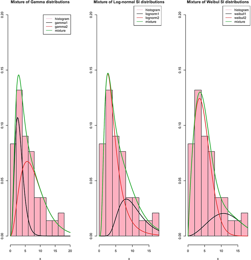
Figure 4. Mixture distribution by the Optim function.

The Log-likelihood, AIC, and BIC values are given in Table 3, and we conclude that the best-fit mixture is given by the mentioned mixture of «Gamma »distributions. This best-fit mixture is better than the MLE.

TABLE 3

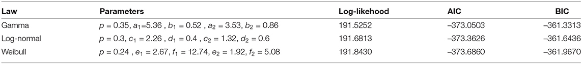
Table 3. Fitted parameter, Log-likehood, AIC, and BIC values with the mixture models.

4.2. The Reproduction Number

In this section, we propose to modify the generation time function provided in the R0 package (refer to [22, 23]) to take into account a mixture modeling framework. Indeed, the choices of series interval estimation models in the R0 package are fixed distributions («Gamma », «Lognormal », and «Weibull ») and do not allow mixture distributions of the serial interval (SI). Furthermore, note that there is no reason for a mixture of Gamma distributions with different non-integer parameters to be Gamma distributed. Thus, using the epidemic incidence curve in Mayotte, we derive a generation time distribution in order to estimate the time varying reproduction number R₀(t) using the non parametric formula in Equation (1) and the best-fit mixture of the SI. The picture in Figure 5 represents the evolution of the time varying reproduction number R₀(t); we make the curve smooth using estimated values.

FIGURE 5

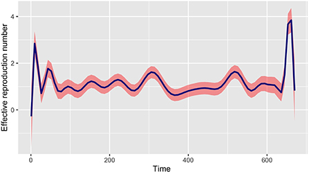
Figure 5. Evolution of the time varying reproductive number in Mayotte from 13 March 2020 to 11 January 2022 with the best-fit mixture of the SI.

The picture in Figure 6 shows not only the evolution of the time-varying reproduction number R(t) with package R0 but also a comparison with our method of estimation in a given period. We can see that at the start of the epidemic the basic reproductive number is around 3. This is consistent with the literature [1, 6, 37] and show that, at the start of the epidemic, an infected individual could contaminate an average of 3 individuals. The public policy measures taken by the authorities and health agency of Mayotte in response to the COVID-19 with a total lockdown on March 17 made it possible to observe a value of this indicator below 1 around the middle of April 2020, showing a temporary decline in the epidemic curve during this period. After then, unfortunately, the dynamic changed over time since the end of the lockdown at the end of May 2020. Subsequently, the Mayotte authorities implemented several measures including non-pharmaceutical intervention measures such as the establishment of curfews, the wearing of mandatory masks in public spaces, and now vaccination. As we can see two other maximum values (explained by the appearance of new variants being more contagious over time) were observed at the end of 2020 and 2021 which justified restriction decisions by the local authorities. Figure 7 shows the relative variation of the reproduction numbers under other mixtures of the SI distributions.

FIGURE 6

Figure 6. Evolution of the time varying reproductive number in Mayotte from 13 March 2020 to 11 January 2022 with a mixture of Log-normal distribution fit of the serial interval (A) and a mixture of Weibull distribution fit of the serial interval (B).

FIGURE 7

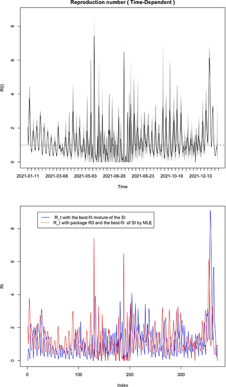
Figure 7. Comparison of our time varying (figure below) reproductive number in Mayotte from 11 January 2021 to 11 January 2022 with the time-varying reproductive number from package R0 (figure above) with the best-fit of the SI by the MLE method.

4.3. Estimates of the Transmission Rates

We give some estimated results of the transmission rates for some given periods such as March 2020, December 2020 and 2021. The following pictures in Figure 8 show the range values of the time-varying transmission rates β(t) using the formula (2) according to the time-varying reproduction numbers R₀(t) and infectious rate γ₁. We make a sensitivity analysis for some values of the asymptotic ratio q. The information we have about the data allow to choose q = 0.2 or q = 0.3. For an infectious ratio r~0.7, one observed transmission rate going around up to 1.6 in March 2020 for a range from 20 % to 30 % of asymptomatic ratio. In the same conditions, the range of transmission rate goes up to 0.9 in December 2020 and up to 2.6 in December 2021. This show strong contact rates in December 2021, which can be explained by the traditional weddings in December in Mayotte. In December 2020, the contact rates were not strong and this can be explained by perhaps less contagiousness of the first variant at this time or by the fact that there were fewer traditional weddings in this same period of 2020 because of the fears of the population.

FIGURE 8

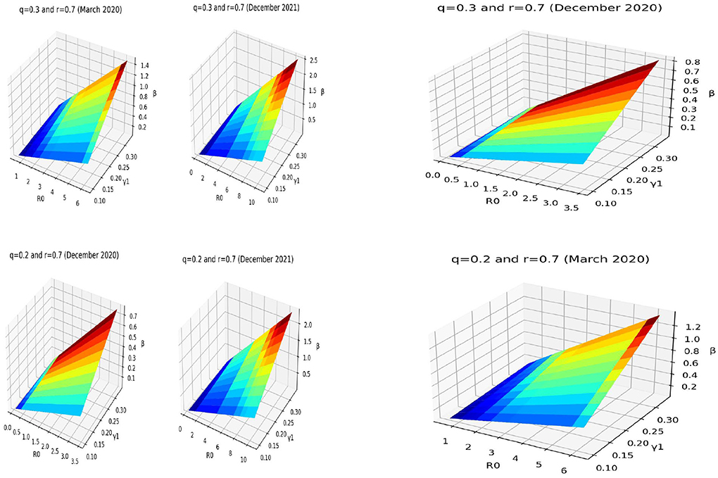
Figure 8. Estimates of the transmission rate with respect to time varying reproduction number R₀(t) and a range of infectious period of symptomatic ${\gamma }_1^{-1}\in (3,10)$.

4.4. Regression and Forecasting Results

The decomposition of the time series of daily hospitalized, intensive care unit, and death cases, allowed us to choose the best models summarized in Table 4. The prediction of the above models is given in Figure 9.

TABLE 4

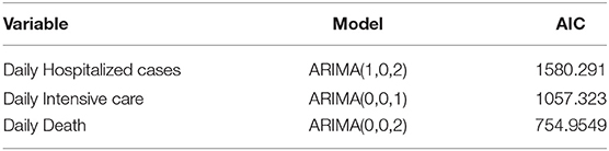
Table 4. Best-fit models and quality measures.

FIGURE 9

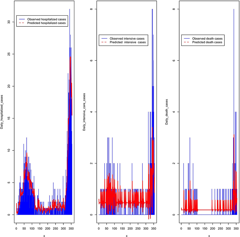
Figure 9. Predicted daily hospitalized, intensive care, and death cases from March 2020 to February 2021.

We analyze in Figure 10, the performance of a polynomial regression model on the cumulative cases with a common R² = 0.998.. The model equations read as follows:

$\begin{array}{l}ICU(t)=81.1352+845.1673I(t)-209.4965I{(t)}^2+161.9409I{(t)}^3\\ -12.5283I{(t)}^4-14.1357I{(t)}^5+13.7583I{(t)}^6.\\ H(t)=500.5775+4597.2940I(t)-1308.7433I{(t)}^2+1107.8621I{(t)}^3\\ -432.4763I{(t)}^4+84.7675I{(t)}^5+51.4808I{(t)}^6.\\ D(t)=28.81127+287.13657I(t)-67.34181I{(t)}^2+64.48529I{(t)}^3\\ -6.12134I{(t)}^4+15.39411I{(t)}^5-18.32997I{(t)}^6-6.64249I{(t)}^7\\ +17.83960I{(t)}^8-4.97188I{(t)}^9-0.32299I{(t)}^{10}+15.86371I{(t)}^{11}\\ -5.82441I{(t)}^{12}-3.39272I{(t)}^{13}+5.66989I{(t)}^{14}-6.59240I{(t)}^{15}\\ -1.09633I{(t)}^{16}+4.11664I{(t)}^{17}+0.66552I{(t)}^{18}.\end{array}$

FIGURE 10

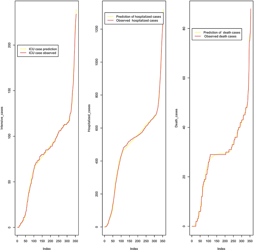
Figure 10. Predicted cumulative intensive care, hospitalized, and death cases from March 2020 to February 2021.

5. Conclusion and Further Studies

In this study, the outbreak dynamics of COVID-19 in Mayotte are discussed through the estimation of the time-varying reproduction number using a non parametric method. To this end, we first make use of statistical methods to fit the probability distribution function which underlines the serial interval distribution of the COVID-19 virus on a given set of data collected on the viral shedding in patients with laboratory-confirmed COVID-19 in He et al. [13]. We propose a modified version in package R0 of the time-varying reproduction number with a mixture estimation model of the serial interval distribution. After that, we considered a deterministic mathematical dynamic epidemic model to estimate the transmission rate parameters by using the Dykman method. In the model, we did not integrate the impact of vaccination because it is well known that vaccination does not prevent being infected, and instead, we introduce a re-infection parameter even though we do not deal in this article with the simulation of the dynamic model. The fit of the transmission rates is done in some given period of observation together with a sensitivity in the asymptotic ratio and infectious ratio between symptomatic and asymptomatic. We discuss some non-pharmaceutical interventions in the evolution of the time-varying reproduction number and the transmission rate coefficients. Any conclusion that can be drawn subject to our assumptions is that mitigation and non-pharmaceutical interventions of the COVID-19 have an impact on the transmission rate parameters. Note also that some conditions can be different in reality, e.g., the infectious rate, the virus mortality rate, and the generation time distribution. This is the limit of our study.

In terms of forthcoming study, we are currently interested in theoretical developments in a context of a cross-mixture in order to improve the estimates considering negative serial interval and α-stables distributions with stochastic Expectation-Maximization algorithm and Bayesian methods, refer to Castillo-Barnes et al. [38] and El Haj et al. [39]. As concerned the regression methods, we are currently working on some other non-parametric forms, refer to Slaoui [40] and Bouzebda and Slaoui [41].

Data Availability Statement

The raw data supporting the conclusions of this article will be made available by the author on reasonable request.

Author Contributions

SM-A performed the conception, preparation, experiment, the statistical analysis of results, and the writing of the present article. YS contributed to the conception. JB contributed to some epidemiological information and interpretation. All authors contributed to the article and approved the submitted version.

Funding

This work was partially funded by the Regional Health Agency (ARS) of Mayotte.

Conflict of Interest

The authors declare that the research was conducted in the absence of any commercial or financial relationships that could be construed as a potential conflict of interest.

Publisher's Note

All claims expressed in this article are solely those of the authors and do not necessarily represent those of their affiliated organizations, or those of the publisher, the editors and the reviewers. Any product that may be evaluated in this article, or claim that may be made by its manufacturer, is not guaranteed or endorsed by the publisher.

Acknowledgments

The authors are indebted to the referees for their valuable comments, criticism and suggestions on a first version of this paper. We also thank the third author involved in the collection and processing of the data.

References

1. Di Domenico L, Pullano G, Sabbatini CE, Boëlle PY, Colizza V. Impact of lockdown on COVID-19 epidemic in Île-de-France and possible exit strategies. BMC Med. (2020) 18:1–13. doi: 10.1186/s12916-020-01698-4

PubMed Abstract | CrossRef Full Text | Google Scholar

2. Salje H, Kiem CT, Lefrancq N, Courtejoie N, Bosetti P, Paireau J, et al. Estimating the burden of SARS-CoV-2 in France. Science. (2020) 369:208–11. doi: 10.1126/science.abc3517

PubMed Abstract | CrossRef Full Text | Google Scholar

3. Dudine P, Hellwig KP, Jahan S, Coady D. A framework for estimating health spending in response to COVID-19. IMF Working Papers (2020).

Google Scholar

4. Di Domenico L, Pullano G, Sabbatini CE, Boëlle PY, Colizza V. Expected impact of reopening schools after lockdown on COVID-19 epidemic in Île-de-France. MedRxiv. (2020). doi: 10.1101/2020.05.08.20095521

CrossRef Full Text | Google Scholar

5. Kucharski AJ, Russell TW, Diamond C, Liu Y, Edmunds J, Funk S, et al. Early dynamics of transmission and control of COVID-19: a mathematical modelling study. Lancet Infect Dis. (2020) 20:553–8. doi: 10.1016/S1473-3099(20)30144-4

PubMed Abstract | CrossRef Full Text | Google Scholar

6. Liu Z, Magal P, Seydi O, Webb G. A COVID-19 epidemic model with latency period. Infect Dis Modell. (2020) 5:323–37. doi: 10.1016/j.idm.2020.03.003

PubMed Abstract | CrossRef Full Text | Google Scholar

7. Liu Z, Magal P, Seydi O, Webb G. Predicting the cumulative number of cases for the COVID-19 epidemic in China from early data. arXiv preprint arXiv:200212298. (2020). doi: 10.1101/2020.03.11.20034314

PubMed Abstract | CrossRef Full Text | Google Scholar

8. Forien R, Pang G, Pardoux É. Epidemic models with varying infectivity. SIAM J Appl Math. (2021) 81:1893–930. doi: 10.1137/20M1353976

CrossRef Full Text | Google Scholar

9. Forien R, Pang G, Pardoux É. Estimating the state of the COVID-19 epidemic in France using a model with memory. R Soc Open Sci. (2021) 8:202327. doi: 10.1098/rsos.202327

PubMed Abstract | CrossRef Full Text | Google Scholar

10. Peter OJ, Qureshi S, Yusuf A, Al-Shomrani M, Idowu AA. A new mathematical model of COVID-19 using real data from Pakistan. Results Phys. (2021) 24:104098. doi: 10.1016/j.rinp.2021.104098

PubMed Abstract | CrossRef Full Text | Google Scholar

11. Abioye AI, Peter OJ, Ogunseye HA, Oguntolu FA, Oshinubi K, Ibrahim AA, et al. Mathematical model of COVID-19 in Nigeria with optimal control. Results Phys. (2021) 28:104598. doi: 10.1016/j.rinp.2021.104598

PubMed Abstract | CrossRef Full Text | Google Scholar

12. Peter OJ, Shaikh AS, Ibrahim MO, Nisar KS, Baleanu D, Khan I, et al. Analysis and dynamics of fractional order mathematical model of COVID-19 in Nigeria using atangana-baleanu operator. Comput Mater Continua. (2021) 66:1823–48. doi: 10.32604/cmc.2020.012314

CrossRef Full Text | Google Scholar

13. He X, Lau EH, Wu P, Deng X, Wang J, Hao X, et al. Temporal dynamics in viral shedding and transmissibility of COVID-19. Nat Med. (2020) 26:672–5. doi: 10.1038/s41591-020-0869-5

PubMed Abstract | CrossRef Full Text | Google Scholar

14. Nishiura H, Linton NM, Akhmetzhanov AR. Serial interval of novel coronavirus (COVID-19) infections. Int J Infect Dis. (2020) 93:284–6. doi: 10.1016/j.ijid.2020.02.060

PubMed Abstract | CrossRef Full Text | Google Scholar

15. Svensson Å. A note on generation times in epidemic models. Math Biosci. (2007) 208:300–11. doi: 10.1016/j.mbs.2006.10.010

PubMed Abstract | CrossRef Full Text | Google Scholar

16. Lehtinen S, Ashcroft P, Bonhoeffer S. On the relationship between serial interval, infectiousness profile and generation time. J R Soc Interface. (2021) 18:20200756. doi: 10.1098/rsif.2020.0756

PubMed Abstract | CrossRef Full Text | Google Scholar

17. Le Cam L. Maximum likelihood: an introduction. Int Stat Rev. (1990) 58:153–71. doi: 10.2307/1403464

CrossRef Full Text | Google Scholar

18. McLachlan GJ, Lee SX, Rathnayake SI. Finite mixture models. Ann Rev Stat Appl. (2019) 6:355–78. doi: 10.1146/annurev-statistics-031017-100325

CrossRef Full Text | Google Scholar

19. Benaglia T, Chauveau D, Hunter DR, Young DS. mixtools: an R package for analyzing mixture models. J Stat Software. (2010) 32:1–29. doi: 10.18637/jss.v032.i06

CrossRef Full Text | Google Scholar

20. Diekmann O, Heesterbeek JAP, Metz JA. On the definition and the computation of the basic reproduction ratio R 0 in models for infectious diseases in heterogeneous populations. J Math Biol. (1990) 28:365–82. doi: 10.1007/BF00178324

PubMed Abstract | CrossRef Full Text | Google Scholar

21. Wallinga J, Lipsitch M. How generation intervals shape the relationship between growth rates and reproductive numbers. Proc R Soc B Biol Sci. (2007) 274:599–604. doi: 10.1098/rspb.2006.3754

PubMed Abstract | CrossRef Full Text | Google Scholar

22. Obadia T, Haneef R, Boëlle PY. The R0 package: a toolbox to estimate reproduction numbers for epidemic outbreaks. BMC Med Inform Decis Making. (2012) 12:1–9. doi: 10.1186/1472-6947-12-147

PubMed Abstract | CrossRef Full Text | Google Scholar

23. Boelle PY, Obadia T, Obadia MT. Package ‘R0'. (2015)

Google Scholar

24. Cori A, Ferguson NM, Fraser C, Cauchemez S. A new framework and software to estimate time-varying reproduction numbers during epidemics. Am J Epidemiol. (2013) 178:1505–12. doi: 10.1093/aje/kwt133

PubMed Abstract | CrossRef Full Text | Google Scholar

25. Cori A, Cauchemez S, Ferguson NM, Fraser C, Dahlqwist E, Demarsh PA, et al. Package ‘EpiEstim' (2021)

Google Scholar

26. Batista M. On the reproduction number in epidemics. J Biol Dyn. (2021) 15:623–34. doi: 10.1080/17513758.2021.2001584

PubMed Abstract | CrossRef Full Text | Google Scholar

27. Demongeot J, Oshinubi K, Rachdi M, Seligmann H, Thuderoz F, Waku J. Estimation of daily reproduction numbers during the COVID-19 outbreak. Computation. (2021) 9:109. doi: 10.3390/computation9100109

PubMed Abstract | CrossRef Full Text | Google Scholar

28. Waku J, Oshinubi K, Demongeot J. Maximal reproduction number estimation and identification of transmission rate from the first inflection point of new infectious cases waves: COVID-19 outbreak example. Math Comput Simulat. (2022) 198:47–64. doi: 10.1016/j.matcom.2022.02.023

PubMed Abstract | CrossRef Full Text | Google Scholar

29. Marill KA. Advanced statistics: linear regression, part I: simple linear regression. Acad Emerg Med. (2004) 11:87–93. doi: 10.1111/j.1553-2712.2004.tb01378.x

PubMed Abstract | CrossRef Full Text | Google Scholar

30. Kumar N, Susan S. COVID-19 pandemic prediction using time series forecasting models. In: 2020 11th International Conference on Computing, Communication and Networking Technologies (ICCCNT). Kharagpur: IEEE (2020). p. 1–7.

Google Scholar

31. Ala'raj M, Majdalawieh M, Nizamuddin N. Modeling and forecasting of COVID-19 using a hybrid dynamic model based on SEIRD with ARIMA corrections. Infect Dis Model. (2021) 6:98–111. doi: 10.1016/j.idm.2020.11.007

PubMed Abstract | CrossRef Full Text | Google Scholar

32. Patibandla RL, Rao BT, Narayana VL. Prediction of COVID-19 using machine learning techniques. In: Deep Learning for Medical Applications with Unique Data. Academic Press (2022). p. 219–31.

PubMed Abstract | Google Scholar

33. Chauhan P, Kumar A, Jamdagni P. Regression analysis of covid-19 spread in india and its different states. medRxiv. (2020). doi: 10.1101/2020.05.29.20117069

CrossRef Full Text | Google Scholar

34. Ekum M, Ogunsanya A. Application of hierarchical polynomial regression models to predict transmission of COVID-19 at global level. Int J Clin Biostat Biom. (2020) 6:27. doi: 10.23937/2469-5831/1510027

CrossRef Full Text | Google Scholar

35. Mizumoto K, Kagaya K, Zarebski A, Chowell G. Estimating the asymptomatic proportion of coronavirus disease 2019 (COVID-19) cases on board the Diamond Princess cruise ship, Yokohama, Japan, 2020. Eurosurveillance. (2020) 25:2000180. doi: 10.2807/1560-7917.ES.2020.25.10.2000180

PubMed Abstract | CrossRef Full Text | Google Scholar

36. McDonald SA, Miura F, Vos ER, van Boven M, de Melker HE, van der Klis FR, et al. Estimating the asymptomatic proportion of SARS-CoV-2 infection in the general population: analysis of nationwide serosurvey data in the Netherlands. Eur J Epidemiol. (2021) 36:735–9. doi: 10.1007/s10654-021-00768-y

PubMed Abstract | CrossRef Full Text | Google Scholar

37. Lekone PE, Finkenstädt BF. Statistical inference in a stochastic epidemic SEIR model with control intervention: Ebola as a case study. Biometrics. (2006) 62:1170–7. doi: 10.1111/j.1541-0420.2006.00609.x

PubMed Abstract | CrossRef Full Text | Google Scholar

38. Castillo-Barnes D, Martínez-Murcia FJ, Ramírez J, Górriz J, Salas-Gonzalez D. Expectation-Maximization algorithm for finite mixture of α-stable distributions. Neurocomputing. (2020) 413:210–6. doi: 10.1016/j.neucom.2020.06.114

CrossRef Full Text | Google Scholar

39. El Haj A, Slaoui Y, Solier C, Perret C. Bayesian Estimation of The Ex-Gaussian Distribution. Stat Optim Inf Comput. (2021) 9:809–19. doi: 10.19139/soic-2310-5070-1251

CrossRef Full Text | Google Scholar

40. Slaoui Y. Recursive nonparametric regression estimation for independent functional data. Stat Sin. (2020) 30:417–37. doi: 10.5705/ss.202018.0069

CrossRef Full Text | Google Scholar

41. Bouzebda S, Slaoui Y. Nonparametric recursive method for kernel-type function estimators for spatial data. StatProbabil Lett. (2018) 139:103–14. doi: 10.1016/j.spl.2018.03.017

CrossRef Full Text | Google Scholar

42. Manou-Abi SM, Balicchi J. Analysis of the COVID-19 epidemic in French overseas department mayotte based on a modified deterministic and stochastic SEIR model. MedRxiv. (2020). doi: 10.1101/2020.04.15.20062752

CrossRef Full Text | Google Scholar