Additive Noise-Induced System Evolution (ANISE)

Introduction

Noise is a major ingredient in most living and artificial thermodynamically open systems. Essentially it is defined as the contrast to signal, that is assumed to be understood or at least known in some detail. Hence the notion of noise is used whenever there is a lack of knowledge on a process, i.e., when it is necessary to describe something unknown or uncontrollable. The relation to chaos and fractals [1] is interesting, which appear to be very complex features of systems if their dynamics are not known. Consequently, noise effects are considered in models if it is mandatory to describe irregular unknown processes. Such processes may be highly irregular and deterministic or random. The following paragraphs do not distinguish these two cases, but mathematical models assume noise to be random.

Since noise represents an unknown process, typically it is identified as a disturbing element that should be removed or compensated. Observed data are supposed to represent a superposition of signals that carry important information on the system under study and noise whose origin is unrelated to the signal source. Moreover, noise may disturb the control of systems, e.g., in aviation engineering, it may induce difficulties in communication systems or acoustic noise may even represent a serious health hazard in industrial work.

However, noise may also be beneficial to the systems dynamics and thus represents an inevitable ingredient. In engineering, for instance, cochlear implants can improve their signal transmission rate by adding noise and thus save electrical power [2]. Biomedical wearables can improve their sensitivity by additive noise [3]. In these applications, noise improves signal transmission by stochastic resonance (SR) [4]. It is well-known that natural systems employ SR to amplify weak signals and thus ensure information transmission [5]. We mention on the side Chaotic Resonance [6], which improves signal transmission by additional chaotic signals and hence demonstrates the similarity between noise and chaos again. Mathematically, systems that exhibit SR have to be driven by a periodic force and additive noise and should exhibit a double-well potential.

Noise is of strong irregular nature and intuition says that additive noise induces irregularity into the stimulated system. Conversely, noise may optimize the systems coherence and thus induce regular behavior. Such an effect is called coherence resonance (CR) [7, 8] and has been demonstrated in a large number of excitable systems, such as chemical systems [9], neural systems [10], nanotubes [11], semi-conductors [12], social networks [13], and the financial market [14]. To describe CR mathematically, the system performs a noise-induced transition between a quiescent non-oscillatory state and an oscillatory state.

Both SR and CR are prominent examples of mechanisms that show a beneficial noise impact. These mechanisms are mathematically specific and request certain dynamical topologies and combination of stimuli, e.g., the presence of two attractors between which the system is moved by additive noise. Other previous mathematical studies have focussed on more generic additive noise-induced transitions, e.g., at bifurcation points. There is much literature on stochastic bifurcations in low-dimensional systems [15–18], spatially-extended systems [19–23], and delayed systems [24–27].

Beyond SR, CR and stochastic bifurcations, additive noise does not only induce stability transitions between states but may tune the system in the stable regime and hence represents an important system parameter. Such an impact is omnipresent in natural systems while it is less prominent and more difficult to observe. Nevertheless, this stochastic facilitation [28] results indirectly to fluctuating, probably random, observations. Examples for such observations are a large variability between repeated measurements [29–31] and strong intrinsic fluctuations in observations [32–34]. To describe such observed random properties, various different fluctuation mechanisms have been proposed, such as deterministic chaotic dynamics [35], heterogeneity [29] or linear high-dimensional dynamics driven by additive noise [36].

To motivate the focus on additive noise in the present work, let us consider the linear stochastic model

$\begin{array}{l}\frac{dx}{dt}=-\gamma x(t)+\alpha x(t)\xi (t)+\beta \eta (t)\end{array}$

with γ, α, β > 0 and spectral white Gaussian distributed noise ξ(t), η(t) both with zero mean and variance D. For multiplicative noise only (α > 0, β = 0), the system ensemble average 〈x〉 obeys [37, 38]

$\begin{array}{l}\frac{d\langle x(t)\rangle }{dt}=\left(-\gamma +\frac{{\alpha }^{2}D}{2}\right)\langle x(t)\rangle .\end{array}$

This shows that the systems origin is a stationary state, whose stability depends on the multiplicative noise variance D. Hence multiplicative noise affects the stability of the system. This is a well-known result [39, 40]. However, multiplicative noise implies that the noise contribution to the system depends on the system activity. This assumption is strong and can not always be validated. Especially in the lack of knowledge how noise couples to the system under study, this assumption appears to be too strong. Hence it is interesting to take a look at additive noise (α = 0, β > 0) whose noise contribution is independent of the system activity. Then

$\begin{array}{l}\frac{d\langle x(t)\rangle }{dt}=-\gamma \langle x(t)\rangle \end{array}$

demonstrating that zero-mean additive noise does not affect the stability of the systems stationary state in the origin. This is also well-established for linear systems. However, some previous stochastic bifurcation studies on the additive noise effect in nonlinear systems have revealed an induced change of stability of the systems stationary state as mentioned above. Moreover, recent diverse studies of additive noise in oscillatory neural systems have revealed that additive noise may tune the systems principal oscillation frequency [41–47]. The present work focusses on a certain class of dynamical differential equation models that exhibit Additive Noise-Induced System Evolution (ANISE) and where the additive noise represents a determinant element. Recently, Powanwe and Longtin [48] have described experimentally observed neural burst activity as an additive noise-controlled process and Powanwe and Longtin [49] have provided conditions under which two additive noise-driven biological systems share optimally their information. Moreover, previous theoretical neural population studies have demonstrated that additive noise can explain intermittent frequency transitions observed in experimental resting state electroencephalographic data [50], dynamical switches between two frequency bands induced by opening and closing eyes in humans [51], and the enhancement of spectral power in the γ-frequency under the anesthetic ketamine [52].

For completeness, it is important to mention quasi-cycle activity [52–55]. Mathematically, this is the linear response of a deterministically stable system to additive noise below a Hopf bifurcation. Without noise, the system would decay exponentially to the systems stable fixed point as a stable focus, whereas the additive noise kicks away the system from the fixed point and thus the system never reaches the fixed point. For long times, the stationary power spectrum of the systems activity is proportional to the noise variance D. This linear relation between spectral power and noise variance has been employed extensively in a large number of previous model studies of experimental spectral power distributions, e.g., in the brain [56, 57]. It is important to point out that the additive noise just scales the global magnitude of the linear systems spectral power distribution, but does not affect selected time scales or frequency bands, e.g., move spectral peaks as observed in the brain [58]. The subsequent sections illustrate how additive noise may affect nonlinear systems in such a way that the systems intrinsic time scales depend on the noise variance.

The following two sections propose extensions of existing studies in ANISE. The first generalizes previous studies of stochastic dynamics in specific nonlinear random networks indicating a perspective to generalize the analysis of such systems. This brief analysis is followed by the novel proposal to extend the stochastic analysis in ANISE by numerical estimates of subgrid-scale models.

Dynamic Random Network Models

To illustrate a possible perspective in ANISE, let us consider a random network of number of nodes N, whose nodes activity obeys

$\begin{array}{l}\frac{d{V}_i(t)}{dt}=g[V_i(t)]+{\displaystyle \sum _{j=1}^N}{K}_{ij}S[V_j(t)]+{\xi }_i(t),\end{array}$

for i = 1, …, N. The additive noise {ξ_i(t)} is uncorrelated between network nodes and Gaussian distributed with zero mean $\sum _{i=1}^N{\xi }_i(t)/N=0$ and variance $D=\sum _{i=1}^N{\xi }_i^2(t)/N$ at every time instance t. The connectivity matrix K is random with non-vanishing mean $\sum _{i,j}{K}_{ij}/N\ne 0$. To gain some insights, at first $g\left[V\right]=-V,S\left[V\right]={\gamma }_{1}V+{\gamma }_2{V}^2+{\gamma }_3{V}^3$ and the network is of Erdös-Rényi-type (ER) [59], i.e., K_ij = 0 with probability 1−c and $K_{ij}=\bar{K}\ne 0$ with connection probability c. In addition, the network is bidirectional with K_ij = K_ji and we choose $\bar{K}=1/Nc$ for convenience. This choice yields a real-valued matrix spectrum and its maximum eigenvalue is λ₁ = 1. As has been shown previously [60], a Galerkin ansatz assists to understand the dynamics of such a network. We define a bi-orthogonal eigenbasis of K with the basis sets {Ψ^(k)}, {Φ^(k)} for which

$\begin{array}{l}{\Psi }^{(k),†}{\Phi }^{(l)}={\delta }_{kl},k,l=1,\dots ,N\end{array}$

with the Kronecker symbol δ_kl, where † denotes the complex conjugate transposition. The eigenspectrum {λ_k} obeys

$\begin{array}{l}\text{K}{\Phi }^{(l)}={\lambda }_l{\Phi }^{(l)},{\Psi }^{(l),†}\text{K}={\lambda }_l{\Psi }^{(l),†}.\end{array}$

It is well-known that the eigenspectrum of symmetric random matrices has an edge distribution and a bulk distribution of eigenvalues [61]. For large ER networks with N → ∞, both distributions are well-separated. The edge distribution consists of the maximum eigenvalue λ₁ with ${\text{Ψ}}_j^{(1)}=1/N,{\Phi }_j^{(1)}=1$ and the bulk distribution obeys the circular law and thus shrinks with λ_k>1 → 0 for N → ∞. Assuming the composition $V_i(t)=\sum _{k=1}^N{\Phi }_i^{(k)}{x}_k(t)$ with time-dependent mode amplitudes x_k(t) and projecting the network activity {V_i} onto the basis {Ψ^(k)}, the mode amplitudes {x_k(t)} obey

$\begin{array}{l}\frac{d{x}_1}{dt}=-x_1+\frac{1}{N}{\displaystyle \sum _{j=1}^N}({\gamma }_1{V}_j+{\gamma }_2{V}_j^2+{\gamma }_3{V}_j^3)\\ +\frac{1}{N}{\displaystyle \sum _{i=1}^N}{\xi }_i& (1)\end{array}$

$\begin{array}{ll}\frac{d{x}_k}{dt}\approx -x_k+{\displaystyle \sum _{i=1}^N}{\text{Ψ}}_i^{(k)}{\xi }_i,k=2,\dots ,N& (2)\end{array}$

Then V_i(t) = x₁(t) + η_i(t) with the Ornstein-Uhlenbeck noise process ${\eta }_i=\sum _{k=2}^N{\Phi }_i^{(k)}{x}_k$ that is Gaussian distributed with ${N}(0,D)$ [60]. Consequently, x₁ describes the mean-field dynamics of the network. Hence, at each node i, V_i exhibits a superposition of mode x₁ and zero-mean fluctuations η_i. For N → ∞ the mode amplitude x₁ obeys

$\begin{array}{l}\frac{d{x}_1}{dt}=-x_1+{\displaystyle {\int }_{-\infty }^{\infty }[{\gamma }_1\left(x_1+w\right)+{\gamma }_2{\left(x_1+w\right)}^2}\\ +{\gamma }_3{\left(x_1+w\right)}^3]p_{ou}\left(w\right)dw& (3)\end{array}$

$\begin{array}{l}={\gamma }_{2}D+({\gamma }_1+3{\gamma }_{3}D-1)x_1+{\gamma }_2{x}_1^2\\ +{\gamma }_3{x}_1^3& (4)\end{array}$

with the Gaussian probability distribution of the Ornstein-Uhlenbeck process $p_{ou}={N}(0,D)$. The mode x₁ is deterministic and the additive noise ξ_i, that drives the network at each node, affects the mean-field network activity tuning the stability of the stationary state x₁ = 0 of the network. Moreover, the systems time scale, which is determined by the linear factor in Equation (4), now depends on the noise variance D.

Figure 1A illustrates the assumptions made. For small networks, the eigenvalue spectrum of the random matrix exhibits a clear gap between the edge spectrum (λ₁ = 1) and the bulk spectrum with λ_k>1 ≈ 0. This spectral gap increases with increasing N. In addition, for small networks the conversion of the sum in (1) to the integral in (3) is a bad approximation, the sum in (1) exhibits strong stochastic fluctuations and hence the network mean fluctuates as well. The larger N, the better is the approximation of the sum by the integral in (3) and the more the dynamics resemble the deterministic mean-field dynamics. Figure 1B presents the systems corresponding potential

$\begin{array}{l}\varphi (x_1)={\gamma }_{2}D{x}_1+\frac{1}{2}({\gamma }_1+3{\gamma }_{3}D-1)x_1^2\\ +\frac{1}{3}{\gamma }_2{x}_1^3+\frac{1}{4}{\gamma }_3{x}_1^4\end{array}$

with dx₁/dt = −dϕ(x₁)/dx₁. For increasing noise variance D, the additive noise merges the stable fixed point (local minimum of ϕ at V ≠ 0) and the unstable fixed point (local maximum of ϕ at V = 0) yielding finally a single stable fixed point (global minimum of ϕ).

FIGURE 1

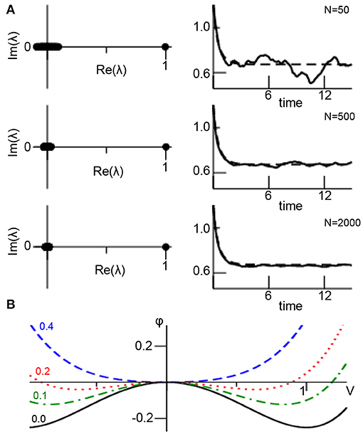
Figure 1. Mean-field description of ANISE. (A) The spectral distribution of random matrix K for different number of network nodes N (left column) and corresponding network mean (solid line, from Equation 1) and mean-field (dashed line, from Equation 4) for comparison (right column). Parameters are K₀ = 1.0, D = 0.1, γ₁ = 2.0, γ₂ = 0.0, γ₃ = −1.0, α = β = 0.0, c = 0.9 and numerical integration time step Δt = 0.03 utilizing the Euler-Maruyama integration method and identical initial values V_i = 1.1 at t = 0 for all parameters. The panels show results for a single network realization, while the variance of results for multiple network realizations is found to be negligible for N ≥ 1, 000 (data not shown). (B) Potential ϕ(V) for different noise variances D.

Although this example illustrates how additive noise induces a stability transition, the underlying network model is too simple to correspond to natural networks. It assumes a large ER-type network that implies a clear separation between edge and bulk spectrum which in turn reflects a sharp unimodal degree distribution. If this spectral gap is not present, then the mean-field activity x₁ impacts on the noise process x_k>1 which renders the analysis much more complex (closure problem). Such a case occurs in most natural networks [62], such as scale-free [63] or small-world networks [64]. Moreover, realistic networks exhibit nonlinear local dynamics g(·) which renders a Galerkin approach as shown above much more complex since it leads to a closure problem as well. As a perspective, new methods have to be developed to treat such cases and to reveal whether ANISE represents the underlying mechanism. In this context, subgrid-scale modeling may be a promising approach as outlined in the subsequent section.

Subgrid-Scale Modeling (SGS)

Most natural systems evolve on multiple spatial and/or temporal scales. Examples are biological systems [65], such as the brain or body tissue, or the earth atmosphere. The latter may exhibit turbulent dynamics whose dynamical details are typically described by the Navier-Stokes equation [66]. The closure problem tells that large scales determine the dynamics of small scales and vice versa. In general, there is rarely a detailed model description of the dynamics on all system scales and the corresponding numerical simulation of all scales is costly. To this end, subgrid-scale modeling [67] chooses a certain model description level and provides a model that captures the effective contribution of smaller scales to the dynamics on the chosen level. The present work proposes, as a perspective, to apply SGS in random network models (cf. previous section) and estimate the subgrid-scale dynamics numerically from full-scale simulations.

For illustration, let us re-consider the example in the previous section. It shows how noise ξ_i on the microscopic scale, i.e., at each node, impacts the evolution of the mesoscopic scale, i.e., spatial mean or mean field. The Galerkin ansatz is successful in the given case for a large family of nonlinear coupling functions S[·] and linear local functions. However, typically complex network systems exhibit local nonlinear dynamics. For illustration reasons, in the following it is g[V] = −V + βV³ and projections onto the eigenbasis of the random matrix yield

$\begin{array}{l}\frac{d{x}_1}{dt}=-x_1+\frac{\beta }{N}{\displaystyle \sum _{i=1}^N{V}_i^3}+\frac{1}{N}{\displaystyle \sum _{j=1}^N(}{\gamma }_1{V}_j\\ +{\gamma }_2{V}_j^2+{\gamma }_3{V}_j^3)+\frac{1}{N}{\displaystyle \sum _{i=1}^N{\xi }_i}& (5)\end{array}$

$\begin{array}{ll}\frac{d{x}_k}{dt}=-x_k+\beta {\displaystyle \sum _{i=1}^N}{\text{Ψ}}_i^{(k)}{V}_i^3+{\displaystyle \sum _{i=1}^N}{\text{Ψ}}_i^{(k)}{\xi }_i& (6)\end{array}$

for k = 2, …, N. It is still V_i = x₁ + η_i with ${\eta }_i=\sum _{k=2}^N{\Phi }_i^{(k)}{x}_k$ as in the previous section, but now the noise term η_i is no Ornstein-Uhlenbeck process anymore due to the nonlinearity in Equation (6). Since the basis {Ψ^(k)} is not known analytically, it is very difficult to gain the stationary probability density function p(·) of η_i.

To address this problem, taking a close look at V_i = x₁ + η_i, x₁ may appear as the mesoscopic activity of the network and η_i may be interpreted as microscopic activity. This new interpretation is motivated by the previous section and stipulates $\sum _{i=1}^n{\eta }_i=0$. Hence, the additional nonlinear local interaction affects the mesoscopic scale dynamics by modulating the microscopic scale dynamics. Now a new subgrid-scale model ansatz assumes that the additional nonlinear local interaction affects the variance of the microscopic scale but retains the microscopic Gaussian distribution shape, i.e., $\eta ~{N}(0,bD)$. Here the additional factor b > 0 captures the impact of the additional nonlinear term $\beta V_i^3$ in g[V]. It represents the subgrid-scale model parameter for the impact of the nonlinear term. For clarification, b = 1 corresponds to β = 0. Inserting this ansatz and V_i = x₁ + η_i into Equation (5) and taking the limit N → ∞

$\begin{array}{l}\frac{d{x}_1}{dt}=F(x_1,b)\\ ={\gamma }_{2}D+({\gamma }_1+3{\gamma }_{3}D-1+3\beta bD)x_1\\ +{\gamma }_2{x}_1^2+({\gamma }_3+\beta )x_1^3& (7)\end{array}$

with a still unknown SGS-factor b. Now let us fit this unknown factor numerically. To this end, numerical simulations of the random network (1) permits to compute the time-dependent network mean V(t_n) with discrete time t_n = nΔt and time step Δt and its temporal derivative ΔV_n = (V(t_n+1)−V(t_n))/Δt. Then minimizing the cost function $C=\sum _{j=1}^T{(\Delta V_n-F\left[V(t_n,b)\right])}^2$ with respect to b yields an optimum SGS-factor b. The corresponding parameter search is done by a Particle Swarm Optimization (PSO) [68, 69]. Figure 2A shows the simulated mesoscopic network mean and the well fit mesoscopic model dynamics (7) for the optimal factor b at different corresponding nonlinearity factors β (numbers given). For each factor β there is an optimal SGS-factor b (cf. Figure 2B), and we can fit numerically a nonlinear dependency of b subjected to β

$\begin{array}{ll}b(\beta )=0.45+0.55e^{6.78\beta }.& (8)\end{array}$

FIGURE 2

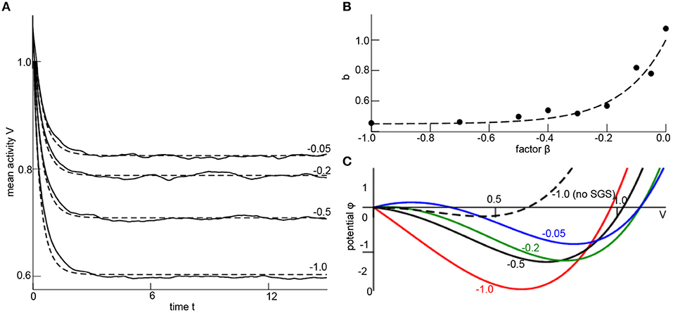
Figure 2. Subgrid-scale modeling. (A) Network mean (solid line) computed from simulations of Equation (1) and mean-field dynamics (7) for different values of β (numbers given) and corresponding optimally estimated factors b. Parameters are V_i(0) = x₁(0) = 1.1, δt = 0.03, K₀ = 1.0, D = 0.33, γ₁ = 2.0, γ₂ = 0.0, γ₃ = −1.0, α = 0.0, N = 1000, c = 0.9 and initial condition V_i(0) = 1.1 ∀i = 1, …, N. The results have been gained for a single network realization, while the variance of results for multiple network realizations is found to be negligible for N ≥ 1000 (data not shown). The optimal factor b has been estimated by employing the Python library pyswarms utilizing the routine single.GlobalBestPSO with optional parameters c₁ = 0.5, c₂ = 0.5, w = 0.3, 60 particles, 50 iterations and taking the best fit over 20 trials. (B) The estimated factor b for different values of β (dots) and the fit polynomial function (dashed line; see Equation 8). (C) The resulting potential ϕ(V) with dϕ/dV = −F[V, b(β)], F is taken from Equation (7), where b is computed from β (numbers given) by Equation (8). The dashed line is plotted for comparison illustrating the impact of the SGS.

This expression is the major result of the SGS modeling since it permits to describe the random network dynamics with nonlinear local interactions by mesoscopic variables with the assistance of a numerical optimization. It is noted that Equation (8) is still valid if other initial conditions for the network simulation are chosen (not shown).

The impact of the nonlinear local interaction on the mean-field is illustrated in Figure 2C, where the potential ϕ(V = x₁) is shown for different factors β implying optimum SGS-factor (different colors in Figure 2C). For comparison, neglecting the SGS model correction (for β = −1.0, dashed line in Figure 2C) yields a potential and dynamical evolution that is different to the true SGS-optimized potential (red line in Figure 2C).

Discussion

A growing number of studies indicate that additive noise represents an important ingredient to systems dynamics. Since such an effect has not been well-studied yet and should be explored in the coming years, it is tempting to name it and pass it the new acronym ANISE. Not only to propose to embrace and name diverse research areas, the present work sketches two future directions of research. Section Dynamic Random Network Models shows in a generalized random network model study that additive noise may change the bifurcation point of the systems stationary state in accordance to previous work on stochastic bifurcations [15, 17, 19, 20]. The example reveals that this effect results from nonlinear and not from linear interactions. In simple words, the additive noise tunes the system by multiplicative noise through the backdoor. Identifying certain system modes, the system exhibits an additive noise effect if some modes are coupled nonlinearly and some of these modes are stochastic. Such modes may be Fourier modes [19], eigenmodes of a coupling matrix [60] (as seen in Section Dynamic Random Network Models) or of a delayed linear operator [70]. Since diverse nonlinear interaction types render a systems analysis complex, Section Subgrid-scale modeling (SGS) proposes a perspective combination of SGS and optimal parameter estimation [71] in the context of ANISE. This combination permits to estimate numerically unknown contributions of subgrid-scale dynamics to larger scales. This may be very useful in studies of high-dimensional nonlinear models, whose dynamics sometimes appears to be untractable analytically.

Data Availability Statement

The raw data supporting the conclusions of this article will be made available by the authors, without undue reservation.

Author Contributions

The author has conceived the work, has performed all simulations and calculations, and has written the manuscript.

Funding

This work has been supported by the INRIA Action Exploratoire A/D Drugs.

Conflict of Interest

The author declares that the research was conducted in the absence of any commercial or financial relationships that could be construed as a potential conflict of interest.

Publisher's Note

All claims expressed in this article are solely those of the authors and do not necessarily represent those of their affiliated organizations, or those of the publisher, the editors and the reviewers. Any product that may be evaluated in this article, or claim that may be made by its manufacturer, is not guaranteed or endorsed by the publisher.

Acknowledgments

The author thanks the reviewer for valuable comments.

References

1. Lasota A, Makey MC, editors. Chaos, Fractals, and Noise - Stochastic Aspects of Dynamics. Vol. 94 of Applied Mathematical Sciences. New York, NY: Springer (1994). doi: 10.1007/978-1-4612-4286-4

CrossRef Full Text | Google Scholar

2. Bhar B, Khanna A, Parihar A, Datta S, Raychowdhury A. Stochastic resonance in insulator-metal-transition systems. Sci Rep. (2020) 10:5549. doi: 10.1038/s41598-020-62537-3

PubMed Abstract | CrossRef Full Text | Google Scholar

3. Kurita Y, Shinohara M, Ueda J. Wearable sensorimotor enhancer for fingertip based on stochastic resonance effect. IEEE Trans Hum Mach Syst. (2013) 43:333–7. doi: 10.1109/TSMC.2013.2242886

CrossRef Full Text | Google Scholar

4. Gammaitoni L, Hanggi P, Jung P. Stochastic resonance. RevModPhys. (1998) 70:223–87. doi: 10.1103/RevModPhys.70.223

CrossRef Full Text | Google Scholar

5. Wiesenfeld K, Moss F. Stochastic resonance and the benefits of noise: from ice ages to crayfish and SQUIDs. Nature. (1995) 373:33–6. doi: 10.1038/373033a0

PubMed Abstract | CrossRef Full Text | Google Scholar

6. Nobukawa S, Nishimura H, Wagatsuma N, Inagaki K, Yamanishi T, Takahashi T. Recent trends of controlling chaotic resonance and future perspectives. Front Appl Math Stat. (2021) 7:760568. doi: 10.3389/fams.2021.760568

CrossRef Full Text | Google Scholar

7. Pikovsky AS, Kurths J. Coherence resonance in a noise-driven excitable system. Phys Rev Lett. (1997) 78:775–8. doi: 10.1103/PhysRevLett.78.775

CrossRef Full Text | Google Scholar

8. Gang H, Ditzinger T, Ning CZ, Haken H. Stochastic resonance without external periodic force. Phys Rev Lett. (1993) 71:807–10. doi: 10.1103/PhysRevLett.71.807

PubMed Abstract | CrossRef Full Text | Google Scholar

9. Beato V, Sendina-Nadal I, Gerdes I, Engel H. Coherence resonance in a chemical excitable system driven by coloured noise. Philos Trans A Math Phys Eng Sci. (2008) 366:381–95. doi: 10.1098/rsta.2007.2096

PubMed Abstract | CrossRef Full Text | Google Scholar

10. Gu H, Yang M, Li L, Liu Z, Ren W. Experimental observation of the stochastic bursting caused by coherence resonance in a neural pacemaker. Neuroreport. (2002) 13:1657–60. doi: 10.1097/00001756-200209160-00018

PubMed Abstract | CrossRef Full Text | Google Scholar

11. Lee CY, Choi W, Han JH, Strano MS. Coherence resonance in a single-walled carbon nanotube ion channel. Science. (2010) 329:1320–4. doi: 10.1126/science.1193383

PubMed Abstract | CrossRef Full Text | Google Scholar

12. Mompo E, Ruiz-Garcia M, Carretero M, Grahn HT, Zhang Y, Bonilla LL. Coherence resonance and stochastic resonance in an excitable semiconductor superlattice. Phys Rev Lett. (2018) 121:086805. doi: 10.1103/PhysRevLett.121.086805

PubMed Abstract | CrossRef Full Text | Google Scholar

13. Tönjes R, Fiore CE, Pereira T. Coherence resonance in influencer networks. Nat Commun. (2021) 12:72. doi: 10.1038/s41467-020-20441-4

PubMed Abstract | CrossRef Full Text | Google Scholar

14. He GYZF, Li JC, Mei DC, Tang NS. Coherence resonance-like and efficiency of financial market. Phys A. (2019) 534:122327. doi: 10.1016/j.physa.2019.122327

CrossRef Full Text | Google Scholar

15. Sri Namachchivaya N. Stochastic bifurcation. Appl Math Comput. (1990) 38:101–59. doi: 10.1016/0096-3003(90)90051-4

CrossRef Full Text | Google Scholar

16. Arnold L, Boxler P. Stochastic bifurcation: instructive examples in dimension one. In: Pinsky MA, Wihstutz V, editors. Diffusion Processes and Related Problems in Analysis, Volume II: Stochastic Flows. Boston, MA: Birkhäuser Boston (1992). p. 241–55. doi: 10.1007/978-1-4612-0389-6_10

CrossRef Full Text | Google Scholar

17. Arnold L. Random Dynamical Systems. Berlin: Springer-Verlag (1998). doi: 10.1007/978-3-662-12878-7

CrossRef Full Text | Google Scholar

18. Xu C, Roberts AJ. On the low-dimensional modelling of Stratonovich stochastic differential equations. Phys A. (1996) 225:62–80. doi: 10.1016/0378-4371(95)00387-8

CrossRef Full Text | Google Scholar

19. Hutt A, Longtin A, Schimansky-Geier L. Additive global noise delays Turing bifurcations. Phys Rev Lett. (2007) 98:230601. doi: 10.1103/PhysRevLett.98.230601

PubMed Abstract | CrossRef Full Text | Google Scholar

20. Hutt A, Longtin A, Schimansky-Geier L. Additive noise-induced Turing transitions in spatial systems with application to neural fields and the Swift-Hohenberg equation. Phys D. (2008) 237:755–73. doi: 10.1016/j.physd.2007.10.013

CrossRef Full Text | Google Scholar

21. Hutt A. Additive noise may change the stability of nonlinear systems. Europhys Lett. (2008) 84:34003. doi: 10.1209/0295-5075/84/34003

PubMed Abstract | CrossRef Full Text | Google Scholar

22. Pradas M, Tseluiko D, Kalliadasis S, Papageorgiou DT, Pavliotis GA. Noise induced state transitions, intermittency and universality in the noisy Kuramoto-Sivashinsky equation. Phys Rev Lett. (2011) 106:060602. doi: 10.1103/PhysRevLett.106.060602

PubMed Abstract | CrossRef Full Text | Google Scholar

23. Bloemker D, Hairer M, Pavliotis GA. Modulation equations: stochastic bifurcation in large domains. Commun Math Phys. (2005) 258:479–512. doi: 10.1007/s00220-005-1368-8

CrossRef Full Text | Google Scholar

24. Guillouzic S, L'Heureux I, Longtin A. Small delay approximation of stochastic delay differential equation. Phys Rev E. (1999) 59:3970. doi: 10.1103/PhysRevE.59.3970

PubMed Abstract | CrossRef Full Text | Google Scholar

25. Lefebvre J, Hutt A, LeBlanc VG, Longtin A. Reduced dynamics for delayed systems with harmonic or stochastic forcing. Chaos. (2012) 22:043121. doi: 10.1063/1.4760250

PubMed Abstract | CrossRef Full Text | Google Scholar

26. Hutt A, Lefebvre J, Longtin A. Delay stabilizes stochastic systems near an non-oscillatory instability. Europhys Lett. (2012) 98:20004. doi: 10.1209/0295-5075/98/20004

CrossRef Full Text | Google Scholar

27. Hutt A, Lefebvre J. Stochastic center manifold analysis in scalar nonlinear systems involving distributed delays and additive noise. Markov Proc Rel Fields. (2016) 22:555–72.

Google Scholar

28. McDonnell MD, Ward LM. The benefits of noise in neural systems: bridging theory and experiment. Nat Rev Neurosci. (2011) 12:415–26. doi: 10.1038/nrn3061

PubMed Abstract | CrossRef Full Text | Google Scholar

29. Eggert T, Henriques DYP, Hart BM, Straube A. Modeling inter-trial variability of pointing movements during visuomotor adaptation. Biol Cybern. (2021) 115:59–86. doi: 10.1007/s00422-021-00858-w

PubMed Abstract | CrossRef Full Text | Google Scholar

30. Fox MD, Snyder AZ, Vincent JL, Raichle ME. Intrinsic fluctuations within cortical systems account for intertrial variability in human behavior. Neuron. (2007) 56:171–84. doi: 10.1016/j.neuron.2007.08.023

PubMed Abstract | CrossRef Full Text | Google Scholar

31. Wolff A, Chen L, Tumati S, Golesorkhi M, Gomez-Pilar J, Hu J, et al. Prestimulus dynamics blend with the stimulus in neural variability quenching. NeuroImage. (2021) 238:118160. doi: 10.1016/j.neuroimage.2021.118160

PubMed Abstract | CrossRef Full Text | Google Scholar

32. Sadaghiani S, Hesselmann G, Friston KJ, Kleinschmidt A. The relation of ongoing brain activity, evoked neural responses, and cognition. Front Syst Neurosci. (2010) 4:20. doi: 10.3389/fnsys.2010.00020

PubMed Abstract | CrossRef Full Text | Google Scholar

33. Krishnan GP, Gonzalez OC, Bazhenov M. Origin of slow spontaneous resting-state neuronal fluctuations in brain networks. Proc Natl Acad Sci USA. (2018) 115:6858–63. doi: 10.1073/pnas.1715841115

PubMed Abstract | CrossRef Full Text | Google Scholar

34. Chew B, Hauser TU, Papoutsi M, Magerkurth J, Dolan RJ, Rutledge RB. Endogenous fluctuations in the dopaminergic midbrain drive behavioral choice variability. Proc Natl Acad Sci USA. (2019) 116:18732–7. doi: 10.1073/pnas.1900872116

PubMed Abstract | CrossRef Full Text | Google Scholar

35. Stringer C, Pachitariu M, Steinmetz NA, Okun M, Bartho P, Harris KD, et al. Inhibitory control of correlated intrinsic variability in cortical networks. eLife. (2016) 5:e19695. doi: 10.7554/eLife.19695

PubMed Abstract | CrossRef Full Text | Google Scholar

36. Sancristobal B, Ferri F, Perucci MG, Romani GL, Longtin A, Northoff G. Slow resting state fluctuations enhance neuronal and behavioral responses to looming sounds. Brain Top. (2021) 35:121–41. doi: 10.1007/s10548-021-00826-4

PubMed Abstract | CrossRef Full Text | Google Scholar

37. Orlandini E. Multiplicative Noise. Unpublished lecture notes on Physics in Complex Systems, University of Padova (2012).

Google Scholar

38. Gardiner CW. Handbook of Stochastic Methods. Berlin: Springer (2004). doi: 10.1007/978-3-662-05389-8

CrossRef Full Text | Google Scholar

39. Sagues F, Sancho JM, Garcia-Ojalvo J. Spatiotemporal order out of noise. RevModPhys. (2007) 79:829–82. doi: 10.1103/RevModPhys.79.829

CrossRef Full Text | Google Scholar

40. Garcia-Ojalvo J, Sancho JM. Noise in Spatially Extended Systems. New York, NY: Springer (1999). doi: 10.1007/978-1-4612-1536-3

CrossRef Full Text | Google Scholar

41. Hutt A, Lefebvre J. Additive noise tunes the self-organization in complex systems. In: Hutt A, Haken H, editors. Synergetics. Encyclopedia of Complexity and Systems Science Series. New York, NY: Springer (2020). p. 183–96. doi: 10.1007/978-1-0716-0421-2_696

CrossRef Full Text | Google Scholar

42. Hutt A, Mierau A, Lefebvre J. Dynamic control of synchronous activity in networks of spiking neurons. PLoS ONE. (2016) 11:e0161488. doi: 10.1371/journal.pone.0161488

PubMed Abstract | CrossRef Full Text | Google Scholar

43. Hutt A, Lefebvre J, Hight D, Sleigh J. Suppression of underlying neuronal fluctuations mediates EEG slowing during general anaesthesia. Neuroimage. (2018) 179:414–28. doi: 10.1016/j.neuroimage.2018.06.043

PubMed Abstract | CrossRef Full Text | Google Scholar

44. Lefebvre J, Hutt A, Knebel JF, Whittingstall K, Murray M. Stimulus statistics shape oscillations in nonlinear recurrent neural networks. J Neurosci. (2015) 35:2895–903. doi: 10.1523/JNEUROSCI.3609-14.2015

PubMed Abstract | CrossRef Full Text | Google Scholar

45. Lefebvre J, Hutt A, Frohlich F. Stochastic resonance mediates the state-dependent effect of periodic stimulation on cortical alpha oscillations. eLife. (2017) 6:e32054. doi: 10.7554/eLife.32054

PubMed Abstract | CrossRef Full Text | Google Scholar

46. Rich S, Hutt A, Skinner FK, Valiante TA, Lefebvre J. Neurostimulation stabilizes spiking neural networks by disrupting seizure-like oscillatory transitions. Sci Rep. (2020) 10:15408. doi: 10.1038/s41598-020-72335-6

PubMed Abstract | CrossRef Full Text | Google Scholar

47. Herrmann CS, Murray MM, Ionta S, Hutt A, Lefebvre J. Shaping intrinsic neural oscillations with periodic stimulation. J Neurosci. (2016) 36:5328–39. doi: 10.1523/JNEUROSCI.0236-16.2016

PubMed Abstract | CrossRef Full Text | Google Scholar

48. Powanwe AS, Longtin A. Determinants of brain rhythm burst statistics. Sci Rep. (2021) 9:18335. doi: 10.1038/s41598-019-54444-z

PubMed Abstract | CrossRef Full Text | Google Scholar

49. Powanwe AS, Longtin A. Mechanisms of flexible information sharing through noisy oscillations. Biology. (2021) 10:764. doi: 10.3390/biology10080764

PubMed Abstract | CrossRef Full Text | Google Scholar

50. Hutt A, Lefebvre J, Hight D, Kaiser H. Phase coherence induced by additive Gaussian and non-Gaussian noise in excitable networks with application to burst suppression-like brain signals. Front Appl Math Stat. (2020) 5:69. doi: 10.3389/fams.2019.00069

CrossRef Full Text | Google Scholar

51. Hutt A, Lefebvre J. Arousal fluctuations govern oscillatory transitions between dominant γ and α occipital activity during eyes open/closed conditions. Brain Topogr. (2021) 35:108–20. doi: 10.1007/s10548-021-00855-z

PubMed Abstract | CrossRef Full Text | Google Scholar

52. Hutt A, Wahl T. Poisson-distributed noise induces cortical γ-activity: explanation of γ-enhancement by anaesthetics ketamine and propofol. J Phys Complex. (2022) 3:015002. doi: 10.1088/2632-072X/ac4004

CrossRef Full Text | Google Scholar

53. Boland RB, Galla T, McKane AJ. How limit cycles and quasi-cycles are related in systems with intrinsic noise. J Stat Mech. (2008) 2008:P09001. doi: 10.1088/1742-5468/2008/09/P09001

CrossRef Full Text | Google Scholar

54. Greenwood PE, Ward LM. Rapidly forming, slowly evolving, spatial patterns from quasi-cycle Mexican Hat coupling. Math Biosci Eng. (2019) 16:6769–93. doi: 10.3934/mbe.2019338

PubMed Abstract | CrossRef Full Text | Google Scholar

55. Powanwe AS, Longtin A. Phase dynamics of delay-coupled quasi-cycles with application to brain rhythms. Phys Rev Res. (2020) 2:043067. doi: 10.1103/PhysRevResearch.2.043067

CrossRef Full Text | Google Scholar

56. Hashemi M, Hutt A, Sleigh J. How the cortico-thalamic feedback affects the EEG power spectrum over frontal and occipital regions during propofol-induced anaesthetic sedation. J Comput Neurosci. (2015) 39:155. doi: 10.1007/s10827-015-0569-1

PubMed Abstract | CrossRef Full Text | Google Scholar

57. Sleigh JW, Voss L, Steyn-Ross ML, Steyn-Ross DA, Wilson MT. Modelling sleep and general anaesthesia. In: Hutt A, editor. Sleep and Anesthesia: Neural correlates in Theory and Experiment. New York, NY: Springer (2011). p. 21–41. doi: 10.1007/978-1-4614-0173-5_2

CrossRef Full Text | Google Scholar

58. Purdon PL, Pierce ET, Mukamel EA, Prerau MJ, Walsh JL, Wong KF, et al. Electroencephalogram signatures of loss and recovery of consciousness from propofol. Proc Natl Acad Sci USA. (2012) 110:E1142-1150. doi: 10.1073/pnas.1221180110

PubMed Abstract | CrossRef Full Text | Google Scholar

59. Erdös P, Rényi A. On random graphs. I. Publ Math. (1959) 6:209–97.

Google Scholar

60. Hutt A, Wahl T, Voges N, Hausmann J, Lefebvre J. Coherence resonance in random Erdos-Renyi neural networks : mean-field theory. Front Appl Math Stat. (2021) 7:697904. doi: 10.3389/fams.2021.697904

CrossRef Full Text | Google Scholar

61. Füredi Z, Komlos J. The eigenvalues of random symmetric matrices. Combinatorica. (1981) 1:233–41. doi: 10.1007/BF02579329

CrossRef Full Text | Google Scholar

62. Yan G, Martinez ND, Liu YY. Degree heterogeneity and stability of ecological networks. J R Soc Interface. (2017) 14:20170189. doi: 10.1098/rsif.2017.0189

PubMed Abstract | CrossRef Full Text | Google Scholar

63. Amaral LAN, Scala A, Barthélémy M, Stanley HE. Classes of small-world networks. Proc Natl Acad Sci USA. (2000) 97:11149–52. doi: 10.1073/pnas.200327197

PubMed Abstract | CrossRef Full Text | Google Scholar

64. Watts DJ, Strogatz SH. Collective dynamics of 'small-world' networks. Nature. (1998) 393:440–2. doi: 10.1038/30918

PubMed Abstract | CrossRef Full Text | Google Scholar

65. Dada JO, Mendes P. Multi-scale modelling and simulation in systems biology. Integr Biol. (2011) 3:86–96. doi: 10.1039/c0ib00075b

PubMed Abstract | CrossRef Full Text | Google Scholar

66. Ghosal S, Moin P. The basic equations for the large eddy simulation of turbulent flows in complex geometry. J Comput Phys. (1995) 118:24–37. doi: 10.1006/jcph.1995.1077

CrossRef Full Text | Google Scholar

67. Germano M, Piomelli U, Moin P, Cabot WH. A dynamic subgrid-scale eddy viscosity model. Phys Fluids. (1991) 3:1760. doi: 10.1063/1.857955

CrossRef Full Text | Google Scholar

68. Freitas D, Guerreiro Lopes L, Morgado-Dias F. Particle swarm optimisation: a historical review up to the current developments. Entropy. (2020) 22:362. doi: 10.3390/e22030362

PubMed Abstract | CrossRef Full Text | Google Scholar

69. Hashemi M, Hutt A, Buhry L, Sleigh JW. Optimal model parameter fit to EEG power spectrum features observed during general anesthesia. Neuroinformatics. (2018) 16:231–51. doi: 10.1007/s12021-018-9369-x

PubMed Abstract | CrossRef Full Text | Google Scholar

70. Lefebvre J, Hutt A. Additive noise quenches delay-induced oscillations. Europhys Lett. (2013) 102:60003. doi: 10.1209/0295-5075/102/60003

CrossRef Full Text | Google Scholar

71. Yuval J, O'Gorman PA. Stable machine-learning parameterization of subgrid processes for climate modeling at a range of resolutions. Nat Commun. (2020) 11:3295. doi: 10.1038/s41467-020-17142-3

PubMed Abstract | CrossRef Full Text | Google Scholar