An Ultraweak Variational Method for Parameterized Linear Differential-Algebraic Equations

1. Introduction

Differential-Algebraic Equations (DAEs) are widely used to model several processes in science, engineering, medicine, and other fields. Theory and numerical approximation methods have intensively been studied in the literature, refer to e.g., [1–4], or [5, 6], which are part of a forum series on DAEs. Quite often, the dimension of DAEs modeling realistic problems is so large that an efficient numerical solution (in particular in realtime environments or within optimal control) is impossible. To address this issue, Model Order Reduction (MOR) techniques have been developed and successfully applied. There is a huge amount of literature, we just mention [7–12].

All methods described in those references address a reduction of the dimension of the system, whereas the temporal discretization is untouched. This article starts at this point. We have been working on space-time variational formulations for (parameterized) partial differential equations (pPDEs) over the last decade. One particular issue has been the stability of the arising discretization which admits tight error-residual relations and thus builds the backbone for model reduction. It turns out that an ultraweak formulation is a right tool to achieve this goal. In [13], we have used this framework for deriving an optimally stable variational formulation of linear time-invariant systems (LTIs). In this article, we extend the ultraweak framework to (parameterized) DAEs and show that this can be combined with system theoretic methods such as Balanced Truncation (BT, [11]) to derive a reduction in the system dimension and time discretization size.

1.1. Differential-Algebraic Equations

Let E, A ∈ ℝ^{n × n}, n ∈ ℕ, be two matrices (E is typically singular), I = (0, T), T > 0, a time interval, $x_0\in {ℝ}^n$ some initial value and f : I → ℝⁿ a given right-hand side. Then, we are interested in the solution x : I → ℝⁿ (the state) of the following initial value problem of a linear DAE with constant coefficients

$\begin{array}{l}E\dot{x}(t)-Ax(t)=f(t),\forall t\in I,x(0)=x_0.\end{array}$

In order to ensure well-posedness (in an appropriate manner), we shall always assume that the initial value x₀ is consistent with the right-hand side f, which means that there exist some ${\widehat{x}}_0\in {ℝ}^n$ such that $E{\widehat{x}}_0-A{x}_0={lim}_{t\to 0+}f(t)$ holds. Finally, we assume that the matrix pencil {E, −A} is regular (i.e., det(λE − A) ≠ 0 for some λ ∈ ℝ) with index ind{E, −A} = : k ∈ ℕ, [14].¹

1.2. Parameterized DAEs (pDAEs)

We are particularly interested in the situation, where one does not only have to solve the above DAE once but several times and highly efficient (e.g., in realtime, optimal control, or cold computing devices) for different data. In order to describe that situation, we are considering a parameterized DAE (pDAE) as follows. For some parameter vector $\mu \in {P}$, ${P}\subset {ℝ}^p$ being a compact set, we are seeking $x_{\mu }:I\to {ℝ}^n$ such that

$\begin{array}{ll}E{\dot{x}}_{\mu }(t)-A_{\mu }{x}_{\mu }(t)=f_{\mu }(t),\forall t\in I,x_{\mu }(0)=x_{0,\mu },& (1.1)\end{array}$

where A_μ, f_μ, and x_0,μ are a parameter-dependent matrix, a right-hand side and an initial condition, respectively, whereas E is assumed to be independent of μ, refer to footnote 5. In order to be able to solve such a pDAE highly efficient for many parameters, it is quite standard to assume that parameters and variables can be separated, refer to e.g., [16]. This is done by assuming a so-called affine decomposition of the data, i.e., E is (for simplicity of exposition) assumed to be parameter-independent and

$\begin{array}{ll}\begin{array}{c}{A}_{\mu }={\displaystyle \sum _{q=1}^{Q_A}}{\vartheta }_q^A(\mu ){Ã}_q,\\ f_{\mu }(t)={\displaystyle \sum _{q=1}^{Q_f}}{\vartheta }_q^f(\mu ){\tilde{f}}_q(t),\\ x_{0,\mu }={\displaystyle \sum _{q=1}^{Q_x}}{\vartheta }_q^x(\mu ){\tilde{x}}_{0,q}.\end{array}& (1.2)\end{array}$

If such a decomposition is not given, we may produce an affinely decomposed approximation by means of the (Discrete) Empirical Interpolation Method [(D)EIM, [17, 18]; refer also to [9] for a system theoretic MOR for such pDAEs]. For well-posedness, we assume that the matrix pencil {E, −A_μ} is regular with index ind{E, −A_μ} = k_μ for all $\mu \in {P}$.

1.3. Reduction to Homogeneous Initial Conditions

Using some standard arguments, eq. (1.1) can be reduced to homogeneous initial conditions x_μ(0) = 0. To this end, construct some smooth extension of the initial data ${\bar{x}}_{\mu }\in C^1{(\bar{I})}^n$, ${\bar{x}}_{\mu }(0)=x_{0,\mu }$. Then, let ${\widehat{x}}_{\mu }:I\to {ℝ}^n$ solve eq. (1.1) with f_μ replaced by ${\widehat{f}}_{\mu }:=f_{\mu }-E{\stackrel{.}{\stackrel{̄}{x}}}_{\mu }+A_{\mu }{\bar{x}}_{\mu }$ and homogeneous initial condition ${\widehat{x}}_{\mu }(0)=0$. Then, $x_{\mu }:={\widehat{x}}_{\mu }+{\bar{x}}_{\mu }$ solves the original problem eq. (1.1). If the pDAE and the extension ${\bar{x}}_{\mu }$ of the initial conditions possess an affine decomposition (for a decomposable ${\bar{x}}_{\mu }$ refer to Section 3.2.2), it is readily seen that the modified right-hand side ${\widehat{f}}_{\mu }$ also admits an affine decomposition. Hence, we can always restrict ourselves to the case of homogeneous initial conditions x_μ(0) = 0, keeping in mind that variable initial conditions can be realized by different right-hand sides.

1.4. Organization of the Material

The remainder of this paper is organized as follows. In Section 2, we derive an ultraweak variational formulation of (1.1) and prove its well-posedness. Section 3 is devoted to a corresponding Petrov-Galerkin discretization and the numerical solution, which is then used in Section 4 to derive a certified reduced model. In Section 5, we report the results of our numerical experiments and end with conclusion and an outlook in Section 6.

2. An Ultraweak Variational Formulation

It is well-known that, for any fixed parameter $\mu \in {P}$, the problem (1.1) admits a unique classical solution $x_{\mu }\in C^{k_{\mu }}{(\bar{I})}^n$ for consistent initial conditions provided that $f_{\mu }\in C^{k_{\mu }-1}{(\bar{I})}^n$, e.g., [3, Lemma 2.8.]. This is a severe regularity assumption, which is one of the reasons why we are interested in a variational formulation. As we shall see, an ultraweak setting is appropriate in order to prove well-posedness, in particular stability. It turns out that this setting is also particularly useful for model reduction of (1.1) with respect to the time variable in the spirit of the reduced basis method, refer to Section 4 below.

2.1. An Ultraweak Formulation of pPDEs

In order to describe an ultraweak variational formulation for the above pDAE, we will review such formulations for parametric partial differential equations (pPDEs). In particular, we are going to follow [19] in which well-posed (ultraweak) variational forms for transport problems have been introduced, refer also to [20–22]. We will then transfer this framework to pDAEs in Section 2.2.

Let Ω ⊂ ℝ^d be some open and bounded domain. We consider a classical² linear operator B_{μ; ∘} on Ω with classical domain

$\begin{array}{l}D(B_{\mu ;\circ })=\{x\in C(\overline{\Omega }):x_{|\partial \Omega }=0,B_{\mu ;\circ }x\in C(\Omega )\}\end{array}$

and aim at solving

$\begin{array}{ll}{B}_{\mu ;\circ }{x}_{\mu }=f_{\mu }\left(\text{pointwise}\right)\text{ on }\Omega ,{x_{\mu }}_{|\partial \Omega }=0.& (2.1)\end{array}$

Note that the definition of B_{μ; ∘} also incorporates essential homogeneous boundary conditions (in the case of a pDAE described below this is the initial condition, which is independent of the parameter). Let $\{B_{\mu ;\circ }^{*},D(B_{\mu ;\circ }^{*})\}$ denote the operator, which is adjoint to {B_{μ; ∘}, D(B_{μ; ∘})}, i.e., $B_{\mu ;\circ }^{*}$ is defined as the formal adjoint of B_{μ; ∘} by $(B_{\mu ;\circ }x,y{)}_{L_2(\Omega )}=(x,B_{\mu ;\circ }^{*}y{)}_{L_2(\Omega )}$ for all $x,y\in C_0^{\infty }(\Omega )$ and its domain $D(B_{\mu ;\circ }^{*})$ which includes the corresponding adjoint essential boundary conditions (so that the above equation still holds true for all x ∈ D(B_{μ; ∘}), $y\in D(B_{\mu ;\circ }^{*})$). Denoting the range of an operator B by R(B), we have B_{μ; ∘} : D(B_{μ; ∘}) → R(B_{μ; ∘}) and $B_{\mu ;\circ }^{*}:D(B_{\mu ;\circ }^{*})\to R(B_{\mu ;\circ }^{*})$. The following assumptions³ turned out to be crucial for ensuring the well-posedness:

(B1) $D(B_{\mu ;\circ }),D(B_{\mu ;\circ }^{*}),R(B_{\mu ;\circ }^{*})\subseteq L_2(\Omega )$ with all embeddings being dense;

(B2) $B_{\mu ;\circ }^{*}$ is injective on $D(B_{\mu ;\circ }^{*})$.

Due to (B2), the injectivity of the adjoint operator, the following quantity

$\begin{array}{l}|||\text{·}{|||}_{\mu }:=\parallel B_{\mu }^{*}·{\parallel }_{L_2(\Omega )}\end{array}$

is a norm on $D(B_{\mu ;\circ }^{*})$, where $B_{\mu }^{*}$ is to be understood as the continuous extension of $B_{\mu ;\circ }^{*}$ onto Y_μ, i.e., $B_{\mu }^{*}:Y_{\mu }\to L_2(\Omega )$, where

$\begin{array}{l}\begin{array}{l}{Y}_{\mu }:={clos}_{|||·{|||}_{\mu }}(D(B_{\mu ;\circ }^{*})),\\ (v,w{)}_{Y_{\mu }}:=(B_{\mu }^{*}v,B_{\mu }^{*}w{)}_{L_2(\Omega )},\\ \parallel v{\parallel }_{Y_{\mu }}^2:=(v,v{)}_{Y_{\mu }}=|||v{|||}_{\mu }^2,\end{array}\end{array}$

is a Hilbert space. Defining the bilinear form

$\begin{array}{l}{b}_{\mu }:L_2(\Omega )\times Y_{\mu }\to ℝ\text{\hspace{1em}by\hspace{1em}}{b}_{\mu }(x,y_{\mu }):=(x,B_{\mu }^{*}{y}_{\mu }{)}_{L_2(\Omega )},\end{array}$

yields an ultraweak form of (2.1): For $f\in Y_{\mu }^{\prime }$⁴, determine x_μ ∈ L₂(Ω) such that

$\begin{array}{ll}{b}_{\mu }(x_{\mu },y_{\mu })=f_{\mu }(y_{\mu })\forall y_{\mu }\in Y_{\mu }.& (2.2)\end{array}$

Well-posedness including optimal stability is now ensured:

Lemma 2.1. Problem eq. (2.2) has a unique solution x_μ ∈ L₂(Ω) and is optimally stable, i.e., ${\gamma }_{\mu }={\beta }_{\mu }={\beta }_{\mu }^{*}=1$, where the continuity constant is defined as

$\begin{array}{l}{\gamma }_{\mu }:={\displaystyle \underset{x\in L_2(\Omega )}{sup}}{\displaystyle \underset{y_{\mu }\in Y_{\mu }}{sup}}\frac{b_{\mu }(x,y_{\mu })}{\parallel x{\parallel }_{L_2(\Omega )}\parallel y_{\mu }{\parallel }_{Y_{\mu }}},\end{array}$

and primal respectively dual inf-sup constants read

$\begin{array}{l}\begin{array}{c}{\beta }_{\mu }:={\displaystyle \underset{x\in L_2(\Omega )}{inf}}{\displaystyle \underset{y_{\mu }\in Y_{\mu }}{sup}}\frac{b_{\mu }(x,y_{\mu })}{\parallel x{\parallel }_{L_2(\Omega )}\parallel y_{\mu }{\parallel }_{Y_{\mu }}},\\ {\beta }_{\mu }^{*}:={\displaystyle \underset{y_{\mu }\in Y_{\mu }}{inf}}{\displaystyle \underset{x\in L_2(\Omega )}{sup}}\frac{b_{\mu }(x,y_{\mu })}{\parallel x{\parallel }_{L_2(\Omega )}\parallel y_{\mu }{\parallel }_{Y_{\mu }}}.\end{array}\end{array}$

Proof: Refer to [19, Proposition 2.1].

2.2. An Ultraweak Formulation of pPDAEs

We are now going to apply the framework of Section 2.1 to the classical form (1.1) of the pDAE. Again, without loss of generality we restrict ourselves to homogeneous initial conditions x_μ(0) = 0, as stated in Section 1.3.

It is immediate that we can generalize ultraweak formulations for scalar-valued functions in L₂(Ω) as above to systems, i.e., $L_2{(\Omega )}^n\equiv L_2(\Omega ;{ℝ}^n)$. For pDAEs, we choose $L_2{(I)}^n$ with the inner product $(·,·{)}_{L_2}\equiv (·,·{)}_{L_2{(I)}^n}$, whereas (·, ·) denotes the Euclidean inner product of vectors. The linear operator {B_{μ; ∘}, D(B_{μ; ∘})} corresponding to (1.1) reads

$\begin{array}{l}\begin{array}{l}{B}_{\mu ;\circ }:=E\frac{d}{dt}-A_{\mu },\\ D(B_{\mu ;\circ }):=\{x\in C^1{(I)}^n\cap C{(\bar{I})}^n:x(0)=0\}.\end{array}\end{array}$

The formal adjoint operator $B_{\mu ;\circ }^{*}$ is easily derived by integration by parts, i.e.,

$\begin{array}{l}(B_{\mu ;\circ }x,y{)}_{L_2}=(E\dot{x}-A_{\mu }x,y{)}_{L_2}=(\dot{x},E^{T}y{)}_{L_2}-(x,A_{\mu }^{T}y{)}_{L_2}\\ =(x(T),E^{T}y(T))-(x(0),E^{T}y(0))-(x,E^T\dot{y}{)}_{L_2}-(x,A_{\mu }^{T}y{)}_{L_2}\\ =(x,-E^T\dot{y}-A_{\mu }^{T}y{)}_{L_2}=:(x,B_{\mu ;\circ }^{*}y{)}_{L_2}\forall x,y\in C_0^{\infty }{(I)}^n,\end{array}$

which shows that

$\begin{array}{l}{B}_{\mu ;\circ }^{*}:=-E^T\frac{d}{dt}-A_{\mu }^T,\\ D(B_{\mu ;\circ }^{*})\equiv C_E^1{(I)}^n:=\{y\in C^1{(I)}^n\cap C{(\bar{I})}^n:y(T)\in \text{ ker}(E^T)\}.& (2.3)\end{array}$

In fact, $(B_{\mu ;\circ }x,y{)}_{L_2}=(x,B_{\mu ;\circ }^{*}y{)}_{L_2}$ for all x ∈ D(B_{μ; ∘}) and $y\in D(B_{\mu ;\circ }^{*})$ since the boundary terms above still vanish due to x(0) = 0 and y(T) ∈ ker(E^T). Moreover, $R(B_{\mu ;\circ })=C^{k_{\mu }-1}{(I)}^n$ and $R(B_{\mu ;\circ }^{*})=C{(I)}^n$.

Lemma 2.2. We have $D(B_{\mu ;\circ }),D(B_{\mu ;\circ }^{*}),R(B_{\mu ;\circ }^{*})\subset L_2{(I)}^n$ with dense embeddings.

Proof: By the definition of $H_0^1{(I)}^n$ and [23, Cor. 7.24] (for H¹(I)ⁿ instead of H¹(I) there, which is a trivial extension), we have

$\begin{array}{l}{C}_0^{\infty }{(I)}^n\subset H_0^1{(I)}^n\subset C{(\bar{I})}^n,\text{ hence},C_0^{\infty }{(I)}^n=C_0^{\infty }{(I)}^n\cap C{(\bar{I})}^n.\end{array}$

With that, $C_0^{\infty }{(I)}^n\subseteq D(B_{\mu ;\circ }),D(B_{\mu ;\circ }^{*}),R(B_{\circ }^{*})\subset L_2{(I)}^n$ is easy to see. Since $C_0^{\infty }{(I)}^n$ is dense in $L_2{(I)}^n$, its supersets $D(B_{\mu ;\circ }),D(B_{\mu ;\circ }^{*}),R(B_{\mu ;\circ }^{*})$ are also dense in $L_2{(I)}^n$.

The above lemma ensures assumption (B1). Next, we consider (B2).

Lemma 2.3. The adjoint operator $\{B_{\mu ;\circ }^{*},D(B_{\mu ;\circ }^{*})\}$ is injective, i.e., for $y_{\mu },z_{\mu }\in D(B_{\mu ;\circ }^{*})$ with $B_{\mu ;\circ }^{*}{y}_{\mu }=B_{\mu ;\circ }^{*}{z}_{\mu }$ we have y_μ = z_μ.

Proof: Setting d_μ: = y_μ − z_μ, we get $B_{\mu ;\circ }^{*}{d}_{\mu }=0$ and

$\begin{array}{l}\begin{array}{c}-E^T{\dot{d}}_{\mu }(t)-A_{\mu }^T{d}_{\mu }(t)=0,\forall t\in I,\\ d_{\mu }(T)=y_{\mu }(T)-z_{\mu }(T)\in ker(E^T).\end{array}\end{array}$

Due to regularity of {E, −A_μ} (and, thus, also of $\{-E^T,-A_{\mu }^T\}$), there are regular matrices P_μ, $Q_{\mu }\in {ℂ}^{n\times n}$, which allow us to transform the problem into Weierstrass-Kronecker normal form, [2, 3], i.e.,

$\begin{array}{l}\begin{array}{l}{P}_{\mu }{E}^T{Q}_{\mu }=\left(\begin{array}{cc}I{d}_m& 0\\ 0& N_{\mu }\end{array}\right),\\ P_{\mu }{A}_{\mu }^T{Q}_{\mu }=\left(\begin{array}{cc}{R}_{\mu }& 0\\ 0& I{d}_{n-m}\end{array}\right),\\ Q_{\mu }^{-1}{d}_{\mu }(t)=\left(\begin{array}{c}{u}_{\mu }(t)\\ v_{\mu }(t)\end{array}\right),\end{array}\end{array}$

where $I{d}_n\in {ℝ}^{n\times n}$ is the identity and N_μ is a nilpotent matrix with nilpotency index k_μ. This yields the equivalent representation

$\begin{array}{ll}{\stackrel{.}{u}}_{\mu }(t)+R_{\mu }{u}_{\mu }(t)=0,\forall t\in I,& (\mathrm{2.4a})\end{array}$

$\begin{array}{ll}{N}_{\mu }{\stackrel{.}{v}}_{\mu }(t)+v_{\mu }(t)=0,\forall t\in I,& (\mathrm{2.4b})\end{array}$

$\begin{array}{lll}{Q}_{\mu }\left(\begin{array}{c}{u}_{\mu }(T)\\ v_{\mu }(T)\end{array}\right)& \in ker(E^T).& (\mathrm{2.4c})\end{array}$

The ODE (2.4a) has the general solution $u_{\mu }(t)=u_{\mu }(T)e^{-R_{\mu }(T-t)}$. By (2.4c), we get

$\begin{array}{l}\begin{array}{l}{E}^T{Q}_{\mu }\left(\begin{array}{c}{u}_{\mu }(T)\\ v_{\mu }(T)\end{array}\right)=0\\ =P_{\mu }{E}^T{Q}_{\mu }\left(\begin{array}{c}{u}_{\mu }(T)\\ v_{\mu }(T)\end{array}\right)=\left(\begin{array}{cc}I{d}_m& 0\\ 0& N_{\mu }\end{array}\right)\left(\begin{array}{c}{u}_{\mu }(T)\\ v_{\mu }(T)\end{array}\right)\\ =\left(\begin{array}{c}{u}_{\mu }(T)\\ N_{\mu }{v}_{\mu }(T)\end{array}\right),\end{array}\end{array}$

Thus, u_μ(T) = 0 and hence $u_{\mu }(t)=u_{\mu }(T)e^{-R_{\mu }(T-t)}=0$ for all t ∈ I.

The initial value problem $N_{\mu }{\stackrel{.}{v}}_{\mu }(t)+v_{\mu }(t)=q_{\mu }(t)$, t ∈ I, v_μ(T) = v_{μ, T} with some $q_{\mu }\in C^{k_{\mu }-1}{(\bar{I})}^{n-m}$ has the unique solution $v_{\mu }(t)=\sum _{i=0}^{k_{\mu }-1}{(-1)}^i{N}_{\mu }^i{q}_{\mu }^{(i)}$, if the initial value v_{μ, T} is consistent, refer to e.g., [1]. We apply this for $q_{\mu }\equiv 0\in C^{k_{\mu }-1}{(\bar{I})}^{n-m}$. Then, by the solution formula, we get v_μ ≡ 0, since the initial value in eq. (2.4c) is by definition trivially consistent. This yields d_μ ≡ 0, i.e., y_μ = z_μ.

Hence, we set $|||·{|||}_{\mu }:=\parallel B_{\mu }^{*}·{\parallel }_{L_2}$ and choose trial and test spaces as

$\begin{array}{l}X:=L_2{(I)}^n,Y_{\mu }:={clos}_{|||·{|||}_{\mu }}\left(C_E^1{(I)}^n\right),\\ b_{\mu }(x,y):=(x,B_{\mu }^{*}y{)}_{L_2},& (2.5)\end{array}$

refer to (2.3) and obtain the following result.

Lemma 2.4. Under the above assumptions, we have for all $\mu \in {P}$ that Y_μ ≡ Y, where

$\begin{array}{l}Y:=H_E^1{(I)}^n:=\{v\in H^1{(I)}^n:v(T)\in ker(E^T)\}.\end{array}$

Proof: Clearly $C_E^1{(I)}^n\subset H_E^1{(I)}^n$, so that Y_μ ⊆ Y for all $\mu \in {P}$. Now, let $y\in Y=H_E^1{(I)}^n$, then, by density, there is a sequence ${(y_{\ell })}_{\ell \in \mathbb{N}}\subset C_E^1{(I)}^n$ such that $\parallel y_{\ell }-y{\parallel }_{H^1{(I)}^n}\to 0$ as ℓ → 0. Since ${P}$ is compact, we have that

$\begin{array}{l}\begin{array}{l}|||y_{\ell }-y{|||}_{\mu }=\left|\right|E^T({\dot{y}}_{\ell }-\dot{y})+A_{\mu }^T(y_{\ell }-y)|{|}_{L_2}\\ \le max\{||E||,||A_{\mu }||\}\left|\right|y_{\ell }-y|{|}_{H^1{(I)}^n}\to 0\end{array}\end{array}$

as ℓ → ∞. Hence, $y\in {clos}_{|||·{|||}_{\mu }}(C_E^1{(I)}^n)=Y_{\mu }$, i.e., Y ⊆ Y_μ.

The latter result must be properly interpreted. It says that Y_μ and Y coincide as sets. However, the norm |||·|||_μ (and thus the topology) still depends on the parameter. The same holds true for the dual space Y′ of Y induced by the L₂-inner product and normed by

$\begin{array}{l}|||f{|||}_{\mu }^{\prime }:={\displaystyle \underset{y\in Y}{sup}}\frac{{(f,y)}_{L_2}}{|||y{|||}_{\mu }}.\end{array}$

In particular, we have a generalized Cauchy-Schwarz inequality ${(f,y)}_{L_2}\le |||f{|||}_{\mu }^{\prime }|||y{|||}_{\mu }$.

Lemma 2.5. Let $f_{\mu }\in Y^{\prime }$. Then, there exists a unique weak solution x_μ ∈ X of

$\begin{array}{ll}{b}_{\mu }(x_{\mu },y)=f_{\mu }(y),\forall y\in Y.& (2.6)\end{array}$

If (1.1) admits a classical solution, then it coincides with x_μ. Moreover, ${\gamma }_{\mu }={\beta }_{\mu }={\beta }_{\mu }^{*}=1$ for the constants defined in Lemma 2.1.

Proof: The existence of a unique solution x_μ ∈ X (as well as ${\gamma }_{\mu }={\beta }_{\mu }={\beta }_{\mu }^{*}=1$) is an immediate consequence of Lemma 2.1. It only remains to show that x_μ satisfying (2.6) is a weak solution to (1.1). To this end, let ${\tilde{f}}_{\mu }\in C{(I)}^n$ be given such that there exists a classical solution ${\tilde{x}}_{\mu }\in C^1{(\bar{I})}^n$ with $B_{\mu ;\circ }{\tilde{x}}_{\mu }(t)={\tilde{f}}_{\mu }(t),\forall t\in I$ and ${\tilde{x}}_{\mu }(0)=0$. Then, define $f_{\mu }\in Y^{\prime }$ by $f_{\mu }(y):=({\tilde{f}}_{\mu },y{)}_{L_2}$. We need to show that the classical solution ${\tilde{x}}_{\mu }$ of (1.1) is also the unique solution of (2.6). First, for $y\in C_E^1{(I)}^n$, integration by parts yields $b_{\mu }({\tilde{x}}_{\mu },y)-f_{\mu }(y)=({\tilde{x}}_{\mu },B_{\mu }^{*}y{)}_{L_2}-f_{\mu }(y)=(B_{\mu ;\circ }{\tilde{x}}_{\mu }-{\tilde{f}}_{\mu },y{)}_{L_2}=0$. Second, let $y\in Y\backslash C_E^1{(I)}^n$, then there is ${({\tilde{y}}_{\ell })}_{\ell \in \mathbb{N}}\subset C_E^1{(I)}^n$ converging to y in Y, i.e., ${lim}_{\ell \to \infty }|||y-{\tilde{y}}_{\ell }{|||}_{\mu }=0$. Then, by the generalized Cauchy-Schwarz inequality

$\begin{array}{l}|b_{\mu }({\tilde{x}}_{\mu },y)-f_{\mu }(y)|=|b_{\mu }({\tilde{x}}_{\mu },y)-f_{\mu }(y)-b_{\mu }({\tilde{x}}_{\mu },{\tilde{y}}_{\ell })+f_{\mu }({\tilde{y}}_{\ell })|\\ =|({\tilde{x}}_{\mu },B_{\mu }^{*}(y-{\tilde{y}}_{\ell }){)}_{L_2}-f_{\mu }(y-{\tilde{y}}_{\ell })|\\ \le \parallel {\tilde{x}}_{\mu }{\parallel }_{L_2}\parallel B_{\mu }^{*}(y-{\tilde{y}}_{\ell }){\parallel }_{L_2}+|||f_{\mu }{|||}_{\mu }^{\prime }|||y-{\tilde{y}}_{\ell }{|||}_{\mu }\\ =\left(\parallel {\tilde{x}}_{\mu }{\parallel }_{L_2}+|||f_{\mu }{|||}_{\mu }^{\prime }\right)|||y-{\tilde{y}}_{\ell }{|||}_{\mu }\to 0\text{ as }\ell \to \infty ,\end{array}$

so that (2.6) holds for ${\tilde{x}}_{\mu }$.

For the ultraweak pDAE (2.6), we need a right-hand side $f_{\mu }\in Y^{\prime }$. However, typically, the right-hand side is given within the context of (1.1) as a function of time, i.e., $g_{\mu }:I\to {ℝ}^n$. Then, we simply define $f_{\mu }\in Y^{\prime }$ by

$\begin{array}{ll}{f}_{\mu }(y):=(g_{\mu },y{)}_{L_2}={\displaystyle {\int }_I}(g_{\mu }(t),y(t))\text{d}t,y\in Y.& (2.7)\end{array}$

3. Petrov-Galerkin Discretization

The next step toward a numerical method for solving an ultraweak operator equation is to introduce finite-dimensional trial and test spaces yielding a Petrov-Galerkin discretization. In this section, we shall first review Petrov-Galerkin methods in general terms and then detail the specification for pDAEs.

3.1. Petrov-Galerkin Method

In order to determine a numerical approximation, we are going to construct an appropriate finite-dimensional trial space $X_{\mu }^{{N}}\subset X=L_2{(I)}^n$ and a parameter-independent test space $Y^{{N}}\subset Y$ of finite (but possibly large) dimension ${N}\in \mathbb{N}$. Then, we are seeking $x_{\mu }^{{N}}\in X_{\mu }^{{N}}$ such that

$\begin{array}{ll}{b}_{\mu }(x_{\mu }^{{N}},y^{{N}})=f_{\mu }(y^{{N}}),\forall y^{{N}}\in Y^{{N}},& (3.1)\end{array}$

which leads to solving a linear system of equations $B_{\mu }^{{N}}{x}_{\mu }^{{N}}=f_{\mu }^{{N}}$ in ${ℝ}^{{N}}$.

Remark 3.1. (a) If one would choose a discretization with $dim(Y^{{N}})>dim(X_{\mu }^{{N}})$, one would need to solve a least squares problem $\left|\right|B_{\mu }^{{N}}{x}_{\mu }^{{N}}-f_{\mu }^{{N}}|{|}^2\to min$.

(b) If one defines the trial space according to $X_{\mu }^{{N}}:=B_{\mu }^{*}{Y}^{{N}}$, then it is easily seen that the discrete problem eq. (3.1) is well-posed and optimally conditioned, [20], i.e.,

$\begin{array}{l}\begin{array}{l}{\gamma }_{\mu }^{{N}}:={\displaystyle \underset{x\in X_{\mu }^{{N}}}{sup}}{\displaystyle \underset{y\in Y^{{N}}}{sup}}\frac{b_{\mu }(x,y)}{\parallel x{\parallel }_{L_2}|||y{|||}_{\mu }}=1,\\ {\beta }_{\mu }^{{N}}:={\displaystyle \underset{x\in X_{\mu }^{{N}}}{inf}}{\displaystyle \underset{y\in Y^{{N}}}{sup}}\frac{b_{\mu }(x,y)}{\parallel x{\parallel }_{L_2}|||y{|||}_{\mu }}=1,\hfill \\ {\beta }_{\mu }^{*,{N}}:={\displaystyle \underset{y\in Y^{{N}}}{inf}}{\displaystyle \underset{x\in X_{\mu }^{{N}}}{sup}}\frac{b_{\mu }(x,y)}{\parallel x{\parallel }_{L_2}|||y{|||}_{\mu }}=1.\hfill \end{array}\end{array}$

(c) The Xu-Zikatanov lemma [24] ensures that the Petrov-Galerkin error is comparable with the error of the best approximation, namely

$\begin{array}{ll}\parallel x_{\mu }-x_{\mu }^{{N}}{\parallel }_{L_2}\le \frac{{\gamma }_{\mu }}{{\beta }_{\mu }^{{N}}}{\displaystyle \underset{v^{{N}}\in X_{\mu }^{{N}}}{inf}}\parallel x_{\mu }-v^{{N}}{\parallel }_{L_2},& (3.2)\end{array}$

so that the Petrov-Galerkin approximation is the best approximation (i.e., an identity) for ${\gamma }_{\mu }={\beta }_{\mu }^{{N}}=1$.

The Petrov-Galerkin framework induces a residual-based error estimation in a straightforward manner. To describe it, let us recall that the residual is defined for some $\tilde{x}\in L_2{(I)}^n$ as

$\begin{array}{l}r(\tilde{x})\in Y^{\prime },r(\tilde{x})\left[y\right]:=f_{\mu }(y)-b_{\mu }(\tilde{x},y),y\in Y.\end{array}$

Then, it is a standard estimate that

$\begin{array}{lll}\left|\right|x_{\mu }-x_{\mu }^{{N}}|{|}_{L_2}& \le \frac{1}{{\beta }_{\mu }}{\displaystyle \underset{y\in Y}{sup}}\frac{b_{\mu }(x_{\mu }-x_{\mu }^{{N}},y)}{|||y{|||}_{\mu }}=\frac{1}{{\beta }_{\mu }}|||r(x_{\mu }^{{N}}){|||}_{\mu }^{\prime }=:{\Delta }_{\mu }^{{N}}& (3.3)\end{array}$

and ${\Delta }_{\mu }^{{N}}$ is a residual-based error estimator. Note that for β_μ = 1 we have an error-residual identity $\left|\right|x_{\mu }-x_{\mu }^{{N}}|{|}_{L_2}=|||r(x_{\mu }^{{N}}){|||}_{\mu }^{\prime }={\Delta }_{\mu }^{{N}}$.

3.2. pPDAE Petrov-Galerkin Discretization

We are now going to specify the above general framework to pDAEs. This means that we need to introduce a suitable discretization in time. We fix a constant time step size Δt: = T/K (i.e., K ∈ ℕ is the number of time intervals) and choose for simplicity equidistant nodes t_k: = kΔt, k = 0, …, K in I. Denote by σ_k, k = 0, …, K piecewise linear splines corresponding to the nodes t_k−1, t_k and t_k+1, refer to Figure 1. For k ∈ {0, K}, the hat functions are restricted to the interval Ī. For realizing a discretization of higher order, one could simply use splines of higher degree.

FIGURE 1

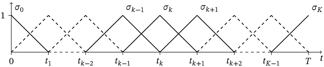
Figure 1. Piecewise linear temporal discretization (hat functions).

As in [20], we start by defining the test space and then construct inf-sup optimal trial spaces. To this end, let d: = dim(ker E^T) and assume that we have a basis {v₁, …, v_d} of ker E^T at hand⁵ and form a matrix $V:=(v_1,...,v_d)\in {ℝ}^{n\times d}$ by arranging the vectors as columns of V. Then, we construct $Y^{{N}}\subset Y=H_E^1{(I)}^n$ independent of the parameter and choose the trial space as $X_{\mu }^{{N}}:=B_{\mu }^{*}{Y}^{{N}}$, which will then guarantee that ${\beta }_{\mu }^{{N}}=1$. We suggest a piecewise linear discretization by

$\begin{array}{l}\begin{array}{l}{Y}^{{N}}:=span\left\{e_i{\sigma }_k:k=0,...,K-1,i=1,...,n\right\}\\ \oplus span\left\{v_i{\sigma }_K:i=1,\dots ,d\right\}\subset Y,\end{array}\end{array}$

where $e_i\in {ℝ}^n$ denotes i-th canonical vector. Then, we set

$\begin{array}{l}{X}_{\mu }^{{N}}:=B_{\mu }^{*}{Y}^{{N}}=span\{-E^T{e}_i{\stackrel{.}{\sigma }}_k-A_{\mu }^T{e}_i{\sigma }_k:k=0,...,K-1,i=1,...,n\}\\ \oplus span\{-A_{\mu }^T{v}_i{\sigma }_K:i=1,\dots ,d\}\subset X=L_2{(I)}^n,\end{array}$

with dimensions ${N}:=dim(X_{\mu }^{{N}})=dim(Y^{{N}})=nK+d$. Then, Lemma 2.5 and Remark 3.1 ensure ${\beta }_{\mu }^{{N}}={\beta }_{\mu }={\gamma }_{\mu }=1$ and thus

$\begin{array}{ll}||x_{\mu }-x_{\mu }^{{N}}|{|}_{L_2}={\displaystyle \underset{v^{{N}}\in X_{\mu }^{{N}}}{inf}}\parallel x_{\mu }-v^{{N}}{\parallel }_{L_2}=|||r(x_{\mu }^{{N}}){|||}_{\mu }^{\prime }={\Delta }_{\mu }^{{N}}.& (3.4)\end{array}$

3.2.1. The Linear System

To construct the discrete linear system $B_{\mu }^{{N}}{x}_{\mu }^{{N}}=f_{\mu }^{{N}}$ we need bases $\left\{{\xi }_1(\mu ),\dots ,{\xi }_{{N}}(\mu )\right\}$ of $X_{\mu }^{{N}}$ and $\left\{{\psi }_1,\dots ,{\psi }_{{N}}\right\}$ of $Y^{{N}}$. The stiffness matrix $B_{\mu }^{{N}}\in {ℝ}^{{N}\times {N}}$ can be computed by ${\left[B_{\mu }^{{N}}\right]}_{j,i}:=b_{\mu }({\xi }_i(\mu ),{\psi }_j)={({\xi }_i(\mu ),B_{\mu }^{*}{\psi }_j)}_{L_2}$. We recall that $X_{\mu }^{{N}}=B_{\mu }^{*}{Y}^{{N}}$, which implies that ${\xi }_i(\mu )=B_{\mu }^{*}{\psi }_i$, so that ${\left[B_{\mu }^{{N}}\right]}_{j,i}={(B_{\mu }^{*}{\psi }_i,B_{\mu }^{*}{\psi }_j)}_{L_2}$ and $B_{\mu }^{{N}}$ is in fact symmetric positive definite.

The right-hand side $f_{\mu }^{{N}}\in {ℝ}^{{N}}$ reads $[f_{\mu }^{{N}}{]}_j:=f_{\mu }({\psi }_j)$. The discrete solution then reads $x_{\mu }^{{N}}:=\sum _{i=1}^{{N}}[x_{\mu }^{{N}}{]}_i{\xi }_i(\mu )$.

Recalling the finite element functions σ_k in Figure 1, we define the inner product matrices for k, ℓ = 0, …, K by

$\begin{array}{l}\begin{array}{c}[K_{\Delta t}{]}_{k,\ell }:=({\stackrel{.}{\sigma }}_k,{\stackrel{.}{\sigma }}_{\ell }{)}_{L_2(I)},\\ [L_{\Delta t}{]}_{k,\ell }:=({\sigma }_k,{\sigma }_{\ell }{)}_{L_2(I)},\\ [O_{\Delta t}{]}_{k,\ell }:=({\stackrel{.}{\sigma }}_k,{\sigma }_{\ell }{)}_{L_2(I)},\end{array}\end{array}$

and subdivide the matrices ${\Pi }_{\Delta t}\in {ℝ}^{(K+1)\times (K+1)}$ for Π_Δt ∈ {K_Δt, L_Δt, O_Δt} according to

$\begin{array}{l}{\Pi }_{\Delta t}=\left(\begin{array}{cc}{\Pi }_{\Delta t}^{1,1}& {\Pi }_{\Delta t}^{1,2}\\ {\Pi }_{\Delta t}^{2,1}& {\Pi }_{\Delta t}^{2,2}\end{array}\right),\begin{array}{c}\begin{array}{l}{\Pi }_{\Delta t}^{1,1}\in {ℝ}^{K\times K},{\Pi }_{\Delta t}^{1,2}\in {ℝ}^{K\times 1},\hfill \\ {\Pi }_{\Delta t}^{2,1}\in {ℝ}^{1\times K},{\Pi }_{\Delta t}^{2,2}\in ℝ.\hfill \end{array}\end{array}\end{array}$

Then, the stiffness matrix also has a block structure

$\begin{array}{l}{B}_{\mu }^{{N}}=\left(\begin{array}{cc}{B}_{\mu }^{1,1}& B_{\mu }^{1,2}\\ B_{\mu }^{2,1}& B_{\mu }^{2,2}\end{array}\right)\in {ℝ}^{{N}\times {N}}\end{array}$

in form of Kronecker products of matrices, i.e., (with $V=(v_1,\dots ,v_d)\in {ℝ}^{n\times d}$ as above),

$\begin{array}{l}{B}_{\mu }^{1,1}=K_{\Delta t}^{1,1}\otimes E{E}^T+O_{\Delta t}^{1,1}\otimes E{A}_{\mu }^T+{(O_{\Delta t}^{1,1})}^T\otimes A_{\mu }{E}^T+L_{\Delta t}^{1,1}\\ \otimes A_{\mu }{A}_{\mu }^T\in {ℝ}^{nK\times nK},\\ B_{\mu }^{1,2}=O_{\Delta t}^{1,2}\otimes E{A}_{\mu }^{T}V+L_{\Delta t}^{1,2}\otimes A_{\mu }{A}_{\mu }^{T}V\in {ℝ}^{nK\times d},\\ B_{\mu }^{2,1}={(O_{\Delta t}^{1,2})}^T\otimes V^T{A}_{\mu }{E}^T+L_{\Delta t}^{2,1}\otimes V^T{A}_{\mu }{A}_{\mu }^T\in {ℝ}^{d\times nK},\\ B_{\mu }^{2,2}=L_{\Delta t}^{2,2}\otimes V^T{A}_{\mu }{A}_{\mu }^{T}V\in {ℝ}^{d\times d}.\end{array}$

For the right-hand side, given some function $f_{\mu }:\bar{I}\to {ℝ}^n$, we obtain a discretization $f_{\mu }^{{N}}\in {ℝ}^{{N}}$ in the sense of (2.7) by $[f_{\mu }^{{N}}{]}_j=\sum _{k=0}^K(f_{\mu }(t_k){\sigma }_k,{\psi }_j{)}_{L_2}$, $j=1,...,{N}$. This means that we discretize f_μ in time by means of piecewise linears. Collecting the sample values of f_μ in one vector, i.e., $f_{\mu ,\Delta t}:=(f_{\mu }(t_0),\dots ,f_{\mu }(t_K){)}^T\in {ℝ}^{n(K+1)}$ we get that

$\begin{array}{l}{f}_{\mu }^{{N}}=F_{\Delta t}^T{f}_{\mu ,\Delta t}\text{where}\\ F_{\Delta t}:=\left(\begin{array}{cc}{L}_{\Delta t}^{1,1}\otimes I{d}_n& L_{\Delta t}^{1,2}\otimes V\\ L_{\Delta t}^{2,1}\otimes I{d}_n& L_{\Delta t}^{2,2}\otimes V\end{array}\right)\in {ℝ}^{n(K+1)\times {N}}\end{array}$

and $I{d}_n\in {ℝ}^{n\times n}$ again denoting the n-dimensional identity matrix.

As already noted above, of course, one could use different discretizations (e.g., higher order or different discretizations for f_μ and the test functions) and we choose the described one just for simplicity.

Due to the Kronecker product structure, the dimension of the system grows rapidly even for moderate n and K. The efficient numerical solution thus requires a solver that takes the specific Kronecker product structure into account in order to accommodate the large system dimension. For similar Kronecker product systems arising from space-time (ultraweak) variational formulations of heat, transport, and wave equations, such specific efficient solvers have been introduced in [21, 25]. However, the solvers in these article are adapted to pPDEs and cannot be used for such kinds of pDAEs we are considering here. Hence, we will devote the development of efficient solvers for ultraweak formulations of pDAEs to future research and refer to Section 6.

3.2.2. Special Case: Fully Linear DAEs

We are going to specify the above general setting to the special case of DAEs with parameter-independent A ≡ A_μ and linear right-hand side which we will call in in the following fully linear DAEs, i.e.,

$\begin{array}{ll}E{\dot{x}}_{\mu }(t)-A{x}_{\mu }(t)=Du(t)+g_{{\mu }_2}(t),t\in I,x_{\mu }(0)=0,& (3.5)\end{array}$

in which the right-hand side depends on the composite parameter μ: = (u, μ₂) and is given in terms of a matrix D ∈ ℝ^n×m, a control u : Ī → ℝ^m, m denoting some input dimension and a function $g_{{\mu }_2}:\bar{I}\to {ℝ}^n$, which arises from the reduction to homogeneous initial conditions, refer to Section 1.3. The initial condition is assumed to be parameterized through g_μ2 by ${\mu }_2\in {{P}}_2\subset {ℝ}^{p_2}$, p₂ ∈ ℕ. In view of (1.2) and Section 1.3, we get

$\begin{array}{l}{g}_{{\mu }_2}(t)={\displaystyle \sum _{q=1}^{Q_x}}{\vartheta }_q^x({\mu }_2)(A{\bar{x}}_q(t)-E{\stackrel{.}{\stackrel{̄}{x}}}_q(t))=:{\displaystyle \sum _{q=1}^{Q_x}}{\vartheta }_q^x({\mu }_2)z_q(t),\end{array}$

where ${\bar{x}}_q\in C^1{(\bar{I})}^n$ are smooth extensions of ${\tilde{x}}_{0,q}$, i.e., ${\bar{x}}_q(0)={\tilde{x}}_{0,q}$, q = 1, …, Q_x.

We view the control and the initial condition (via g_μ2) as parameters, i.e., f_μ(t) = Dμ₁(t) + g_μ2(t), μ = (μ₁, μ₂), which means that the parameter set would be infinite-dimensional and needs to be discretized. Using the same kind of discretization as above, we can use the samples of the control as a parameter, i.e.,

$\begin{array}{l}{\mu }_1:=(u(t_0),...,u(t_K){)}^T\in {{P}}_1={ℝ}^{p_1},p_1=m(K+1),\end{array}$

and similar to the initial condition $z_q:=(z_q(t_0),...,z_q(t_K){)}^T\in {ℝ}^{n(K+1)}$, q = 1, …, Q_x. Then, we get

$\begin{array}{l}{f}_{\mu }^{{N}}=F_{\Delta t}^T(D\otimes I{d}_{K+1}){\mu }_1+{\displaystyle \sum _{q=1}^{Q_x}}{\vartheta }_q^x({\mu }_2)F_{\Delta t}^T{z}_q,\end{array}$

so that the parameter dimension is p = p₁ + p₂ = m(K + 1) + p₂, which might be large. The right-hand side $f_{\mu }^{{N}}$ thus also admits an affine decomposition with Q_f = p₁ + Q_x = m(K + 1) + Q_x terms. However, this number might be an issue concerning efficiency if K is large, we nevertheless have $Q_f\ll {N}$ if m ≪ n.

Moreover, in the fully linear case, the matrix A_μ ≡ A is independent of the parameter, which means (among other facts) that trial and test spaces are parameter-independent, as sets and also with respect to their topology. Note that this is the most common case for system theoretic MOR methods (like BT), which are often even restricted to this case, [10, 11], with the exception [9]. Our setting seems more flexible in this regard and fully linear DAEs are just a special case.

4. Model Order Reduction: The Reduced Basis Method

The Reduced Basis Method (RBM) is a model order reduction technique that has originally been constructed for parameterized partial differential equations (pPDEs), refer to e.g., [7, 16, 26]. In an offline training phase, a reduced basis of size $N\ll {N}$ is constructed (typically in a greedy manner, refer to Algorithm 1 below) from sufficiently detailed approximations for certain parameter samples (also called truth approximations or snapshots), which are computed e.g., by a Petrov-Galerkin method as described above. In particular, ${N}$ is assumed to be sufficiently large in order to ensure that $x_{\mu }^{{N}}$ is (at least numerically) indistinguishable from the exact state x_μ, which explains the name truth. As long as an efficient solver for the detailed problem is available, we may assume that the snapshots can be computed in ${O}({N})$ complexity.

Given some parameter value μ, the reduced approximation x_N(μ)⁶ is then computed by solving a reduced system of dimension N. As a result of the affine decomposition (1.2), several quantities for the reduced system can be precomputed and stored so that a reduced approximation is determined in ${O}(N^3)$ operations, independent of ${N}$ (which is called online efficient). Moreover, an a posteriori error estimator Δ_N(μ) guarantees a certification in terms of an online efficiently computable upper bound for the error, i.e., $\left|\right|x_{\mu }^{{N}}-x_N(\mu )|{|}_{L_2}\le {\Delta }_N(\mu )$.

We are going to use this framework for pDAEs of the form (1.1). Model reduction of (1.1) may be concerned (at least) with the following quantities

• Size n of the system,

• Dimension K of the temporal discretization,

where we have in mind to solve (1.1) extremely fast for several values of the parameter μ. As mentioned earlier, the first issue has extensively been studied in the literature e.g., by system theoretic methods, in particular for fully linear DAEs (3.5). This can be done independently from the subsequent reduction with respect to K (both for parameterized and non-parameterized versions), so we even might assume that such Model Order Reduction (MOR) techniques have already been applied in a preprocessing step. We mention [9] a system theoretic MOR for parameter-dependent DAEs. Here, we are going to consider the reduction with respect to time using the RBM based upon a variational formulation with respect to the time variable.

We restrict ourselves to the reduction of the fully linear case of (3.5) as it easily shows how the RBM-inspired model reduction can be combined with existing system theoretic approaches to reduce the size of the system (e.g., in a preprocessing step). In the fully linear case, the matrix A_μ ≡ A and, hence, all operators and bilinear forms on the left-hand side are parameter-independent. This implies in addition that the ansatz space $X_{\mu }^{{N}}\equiv X^{{N}}$ and the norm |||·|||_μ ≡ |||·||| inducing the topology on the test space are parameter-independent as well, which of course simplifies the framework. However, parameter-dependent matrices A_μ can be treated similar to the RBM for ultraweak formulations of pPDEs as described e.g., in [20–22]. We further note that the RB approach also allows the treatment of more general pDAEs and is not restricted to fully linear systems (3.5), in particular with respect to the right-hand side.

The idea of the RBM can be described as follows: One determines sample values

$\begin{array}{l}{S}_N:=\{{\mu }^{(1)},...,{\mu }^{(N)}\}\subset {P}\end{array}$

of the parameters in an offline training phase by a greedy procedure described in Algorithm 1 below. Then, for each μ ∈ S_N, we determine a sufficiently detailed snapshot $x_{\mu }^{{N}}\in X^{{N}}$ by the ultraweak Petrov-Galerkin discretization as in Section 3.2 and obtain a reduced space of dimension N by setting

$\begin{array}{l}{X}_N:=span\{x_{\mu }^{{N}}:\mu \in S_N\}=:span\{{\zeta }_1,...,{\zeta }_N\}\subset X^{{N}}.\end{array}$

We also need a reduced test space for the Petrov-Galerkin method. Recalling that the operator is parameter-independent here (B_μ ≡ B) and also the trial space $X^{{N}}$ is independent of μ, we can easily identify the optimal test space. In fact, for each snapshot, there exists a unique $y_{\mu }^{{N}}\in Y^{{N}}$ such that $x_{\mu }^{{N}}=B^{*}{y}_{\mu }^{{N}}$. Then, we define

$\begin{array}{l}{Y}_N:=span\{y_{\mu }^{{N}}:\mu \in S_N\}=:span\{{\eta }_1,...,{\eta }_N\}\subset Y^{{N}}.\end{array}$

Then, given a new parameter value $\mu \in {P}$, one determines the reduced approximation x_N(μ) ∈ X_N by solving (recall that here b_μ ≡ b).

$\begin{array}{l}b(x_N(\mu ),y_N)=f_{\mu }(y_N)\text{for all }{y}_N\in Y_N.\end{array}$

If $N\ll {N}=nK+d$, we can compute a reduced approximation with significantly less effort as compared to the Petrov-Galerkin (or a time-stepping) method. To determine the reduced approximation x_N(μ), we have to solve a linear system of the form B_Nx_N(μ) = f_N(μ), where the stiffness matrix is given by [B_N]_j,i = b(ζ_i, η_j), i, j = 1, …, N, recalling that the bilinear form is parameter-independent. Hence, $B_N\in {ℝ}^{N\times N}$ can be computed and stored in the offline phase. For the right-hand side, we use the affine decomposition (1.2) and get ${\left[f_N(\mu )\right]}_j=\sum _{q=1}^{Q_f}{\vartheta }_g^f(\mu ){({\tilde{f}}_q,{\eta }_j)}_{L_2}$. The quantities ${({\tilde{f}}_q,{\eta }_j)}_{L_2}$ can be precomputed and stored in the offline phase so that f_N(μ) is computed online efficiently in ${O}(Q_{f}N)$ operations. Obtaining the coefficient vector x_N(μ), the reduced approximation results in $x_N(\mu )=\sum _{i=1}^N{\left[x_N(\mu )\right]}_i{\zeta }_i$. Note that the matrix B_N is typically densely populated so the numerical solution requires in general ${O}(N^3)$ operations.

The announced greedy selection of the samples is based upon the residual error estimate (here identity) ${\Delta }_{\mu }^{{N}}$ in (3.3) respectively (3.4) for the reduced system described as follows: In a similar manner as deriving ${\Delta }_{\mu }^{{N}}$ in (3.3), we get a residual based error estimator for the reduced approximation

$\begin{array}{l}\begin{array}{l}\left|\right|x_{\mu }^{{N}}-x_N(\mu )|{|}_{L_2}\le \frac{1}{{\beta }^{{N}}}{\displaystyle {sup}_{y\in Y^{{N}}}}\frac{b(x_{\mu }^{{N}}-x_N(\mu ),y)}{|||y|||}\\ =\frac{1}{{\beta }^{{N}}}|||r(x_N(\mu )){|||}^{\prime }\\ =:{\Delta }_N(\mu ),\end{array}\end{array}$

since the bilinear form and the norm in Y are parameter-independent here. Hence, the inf-sup constant is parameter-independent as well, i.e., ${\beta }_{\mu }^{{N}}\equiv {\beta }^{{N}}$ and it is unity by Remark 3.1, so that

$\begin{array}{ll}\left|\right|x_{\mu }^{{N}}-x_N(\mu )|{|}_{L_2}=|||r(x_N(\mu )){|||}^{\prime }={\Delta }_N(\mu ).& (4.1)\end{array}$

Its computation can be done in an online efficient manner in ${O}(N)$ operations by determining Riesz representations in the offline phase, refer to [7, 16, 26]. We use this error identity in the greedy method in Algorithm 1 below.

ALGORITHM 1

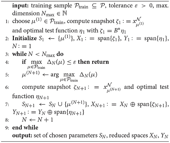
Algorithm 1. (Weak) Greedy method

5. Numerical Experiments

In this section, we report on the results of some of our numerical experiments. Our main focus is on the numerical solution of the ultraweak form of the pDAE, the error estimation, and the quantitative reduction. We solve the arising linear systems for the Petrov-Galerkin and the reduced system by MATLAB's backslash operator, refer also to our remarks in Section 6 below. The code for producing the subsequent results is available via https://github.com/mfeuerle/Ultraweak_PDAE.

5.1. Serial RLC Circuit

We start with a standard problem which (in some cases) admits a closed formula for the analytical solution. This allows us to monitor the exact error and comparison with standard time-stepping methods. Our particular interest is the approximation property of the ultraweak approach, which is an L₂-approximation.

The serial RLC circuit consists of a resistor with resistance R, an inductor with inductance L, a capacitor with capacity C and a voltage source fed by a voltage curve f_VS : Ī → ℝ. Kirchhoff's circuit and further laws from electrical engineering yield a DAE with the data.

$\begin{array}{l}E=\left(\begin{array}{cccc}1& 0& 0& 0\\ 0& 1& 0& 0\\ 0& 0& 0& 0\\ 0& 0& 0& 0\end{array}\right),A=\left(\begin{array}{cccc}0& 0& L^{-1}& 0\\ C^{-1}& 0& 0& 0\\ R& 0& 0& -1\\ 0& 1& 1& 1\end{array}\right),x=\left(\begin{array}{c}{x}_I\\ x_{V_C}\\ x_{V_L}\\ x_{V_R}\end{array}\right),f=\left(\begin{array}{c}0\\ 0\\ 0\\ -f_{V_S}\end{array}\right),\end{array}$

whose index is k = 1. The solution x consists of the electric current x_I and the voltages at the capacitor x_VC, at the inductor x_VL, and the resistor x_VR.

5.1.1. Convergence of the Petrov-Galerkin Scheme

In Figure 2, we compare the exact solution with approximations generated by a standard time-stepping scheme (using MATLAB's fully implicit variable order solver with adaptive step size control ode15i, [27]) and by our ultraweak formulation from Section 3.2. We choose two specific examples for f_VS, namely a smooth and a discontinuous one,

$\begin{array}{l}{f}_{V_S}^{\text{smooth}}(t):=sin\left(\frac{4\pi }{T}t\right),f_{V_S}^{\text{disc}}(t):=sign\left(cos\left(\frac{4\pi }{T}t\right)\right).\end{array}$

For the smooth right-hand side (left graph in Figure 2), both ode15i and the ultraweak method give good results. Concerning the deviations for the ultraweak approach at the start and end time, we recall that the ultraweak form yields an approximation in L₂ so pointwise comparisons are not necessarily meaningful.

FIGURE 2

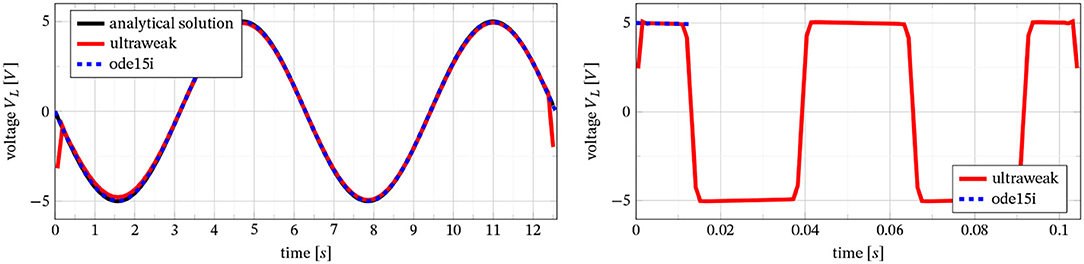
Figure 2. Serial RLC circuit, the exact voltage at the inductor; comparison of time-stepping (ode15i – blue) and ultraweak (red) approximation for smooth $f_{V_S}^{\mathrm{\text{smooth}}}$ (left, including analytical solution) and discontinuous $f_{V_S}^{\mathrm{\text{disc}}}$ (right) right-hand side.

In the discontinuous case, the existence of a classical solution cannot be guaranteed by the above arguments. In particular, there is no closed solution formula. As we see in the right graph in Figure 2, ode15i stops at the first jump. This is to be expected, since $f_{V_S}^{\mathrm{\text{disc}}}\notin C^0(\bar{I})$, so that the solution lacks sufficient regularity to guarantee convergence of a time-stepping scheme like ode15i (even though it is an adaptive variable order method). We could resolve the jumps even better by choosing more time steps K, while ode15i still fails. We conclude that the ultraweak method also converges for problems lacking regularity.

5.1.2. Convergence Rate

Next, we investigate the rate of convergence for the ultraweak form. To that end, we use $f_{V_S}^{\mathrm{\text{smooth}}}$, since the analytical solution x* is known and we can thus compute the relative error $\parallel x^{*}-x^{{N}}{\parallel }_{L_2}/\parallel x^{*}{\parallel }_{L_2}$. Using the lowest order discretization as mentioned above (namely piecewise linear test functions ψ_j, which yield discontinuous trial functions $B^{*}{\psi }_i$), we can only hope for the first order (with respect to the number of time steps K), which we see in Figure 3 and was observed in all cases we considered. We obtain higher order convergence by choosing test functions of higher order, provided the solution has sufficient smoothness.

FIGURE 3

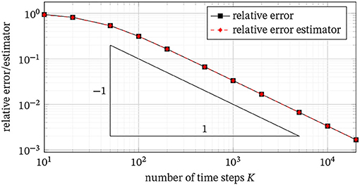
Figure 3. Relative error $\parallel x^{*}-x^{{N}}{\parallel }_{L_2}/\parallel x^{*}{\parallel }_{L_2}$ and relative error estimator ${\Delta }^{{N}}/\parallel x^{*}{\parallel }_{L_2}$ with respect to the analytical solution x^* for increasing numbers of time steps K.

Moreover, we compare the exact relative error with our error estimator (refer to Section 3.1). Figure 3 shows a perfect matching confirming the error-residual identity (3.4) also for the numerically computed error estimator.

5.2. Time-Dependent Stokes Problem

In order to investigate the quantitative performance of the model reduction, we consider a problem, which has often been used as a benchmark, [28–31], namely the time-dependent Stokes problem on the unit square (0, 1)², discretized by a finite volume method on a uniform, staggered grid for the spatial variables with n unknowns, [31], where we choose n = 644. The arising homogeneous fully linear DAE with output function y : I → ℝ takes the form (3.5),

$\begin{array}{ll}E\dot{x}(t)-Ax(t)=Du(t)+g(t),t\in I,x(0)=0,& (\mathrm{5.1a})\end{array}$

$\begin{array}{ll}y(t)=Cx(t),& (\mathrm{5.1b})\end{array}$

where C ∈ ℝ^{1 × n} is an output matrix, D ∈ ℝ^n×1 is the control matrix, and u : I → ℝ is a control, which serves as a parameter μ ≡ u as described in Section 3.2.2 above. We use a parameter-independent initial condition, so that g_μ ≡ g and Q_x = 1.

In order to combine system theoretic model reduction with the RBM from Section 4, we use the system theoretic model order reduction package [28]. In particular, we use Balanced Truncation (BT) from [30] during a preprocessing step to reduce the above system of dimension n to a system

$\begin{array}{ll}\widehat{E}\stackrel{.}{\widehat{x}}(t)-\widehat{A}\widehat{x}(t)=\widehat{D}u(t)+ĝ(t),t\in I,\widehat{x}(0)=0,& (\mathrm{5.2a})\end{array}$

$\begin{array}{ll}y(t)=Ĉ\widehat{x}(t),& (\mathrm{5.2b})\end{array}$

with $\widehat{E},\widehat{A}\in {ℝ}^{\widehat{n}\times \widehat{n}}$, $\widehat{D}\in {ℝ}^{\widehat{n}\times 1}$, $Ĉ\in {ℝ}^{1\times \widehat{n}}$ as well as $\widehat{x},ĝ:\bar{I}\to {ℝ}^{\widehat{n}}$ and $\widehat{n}\ll n$. We note that the resulting reduced system typically provides regular matrices $\widehat{E},\widehat{A}$. Then, the reduced system is an LTI system, which is an easier problem than a DAE and in fact a special case. Hence, our presented approach is still valid, even though designed for pDAEs. For an ultraweak formulation of LTI systems, we refer to [13].

Remark 5.1. We use the RBM here for deriving a certified reduced approximation of the state x. If we would want to control the output y along with a corresponding error estimator ${\Delta }_N^y$, it is fairly standard in the theory of RBM to use a primal-dual approach with a second (dual) reduced basis, e.g., [16, 26]. For simplicity of exposition, we leave this to future study and compute the output from the state by $Ĉ\widehat{x}(t)$, respectively Cx(t).

5.2.1. Discretization of the Control Within the RBM

Since we use a variational approach, we are in principle free to choose any discretization for the control (we only need to compute inner products with the test basis functions). We tested piecewise linear discretizations as described in Section 3.2 for different step sizes T/K_u, where K_u might be different from K, which we choose for discretizing the state. Doing so, the parameter reads $\mu =(u(t_0),\dots ,u(t_{K_u}){)}^T\in {P}\equiv {ℝ}^{K_u+1}$, i.e., the parameter dimension is p = K_u + 1, which might be large. Large parameter dimensions are potentially an issue for the RBM since the curse of dimension occurs. Hence, we investigate if we can reduce K_u within the RBM.

In order to answer this question, we apply Algorithm 1 to the time-dependent Stokes problem (5.1a) (without BT) setting ε = 0, N_max = Q_f from (1.2) (i.e., Q_f = p + 1 for the fully linear system with parameter-independent initial value) and ${{P}}_{\mathrm{\text{train}}}$ consisting of 500 random vectors for K_u ≡ K ∈ {75, 150, 300}, i.e., ${N}=48524,96824,193424$, where d = 224. For these three cases, we investigate the max greedy training error, i.e., ${max}_{\mu \in {{P}}_{\mathrm{\text{train}}}}{\Delta }_N(\mu )$. The results in Figure 4 show an exponential decay with respect to the dimension N of the reduced system with slower decay as K grows. This is to be expected as the discretized control space is much richer for growing K_u and the reduced model has to be able to represent this variety. However, in relative terms (i.e., reduced size N compared with full size K), we see that the compression rates are almost the same. This shows that the RBM can effectively reduce the system no matter how strong the influence of the control on the state is. It is expected that this potential is even more pronounced if a primal-dual RBM is used for the output.

FIGURE 4

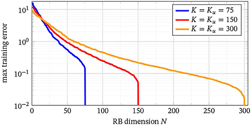
Figure 4. Maximal greedy training error $\underset{\mu \in {{P}}_{\mathrm{\text{train}}}}{max}{\Delta }_N(\mu )$ for different time resolutions K_u = K ∈ {75, 150, 300} over the reduced dimension N.

Next, we note that for A ≡ A_μ as (5.1a), the reduced model is always exact for N ≥ Q_f, which explains the drop off of the curves in Figure 4. For fully linear DAEs, a reduced model with N ≥ Q_f = K_u + 2 is always exact. Hence, if m ≪ n (here m = 1 ≪ 644 = n), we obtain an exact reduced model of dimension $N=Q_f=p+Q_x=m(K_u+1)+1\ll nK+d=:{N}$. Even though this seems to be attractive for low-dimensional outputs, we stress the fact that the reduced dimension still depends on the temporal dimension K_u, which might be large. Hence, a combination of a possibly small discretization of the control and an RBM seems necessary.

Let us comment on the error decay of the RBM produced by the greedy method using the error estimator derived from the ultraweak formulation of the pDAE. We obtain exponential decay of the error, which in fact shows the potential of the RBM. The question whether a given pDAE permits a fast decay of the greedy RBM error is well-known to be linked to the decay of the Kolmogorov N-width, [7, 16, 22], which is a property only of the problem at hand. In other words, if a pDAE can be reduced with respect to time, the greedy method will detect this.

The results in Figure 4 use K_u = K. The next question is how the error behaves for K_u < K. To this end, we determine the error in the state with respect to the full resolution, i.e., we compare the state derived from the control with K_u degrees of freedom with the state of the fully resolved control. In Figure 5, we display errors for different values for K. We obtain fast convergence, which again shows the significant potential for a reduced temporal discretization of the control.

FIGURE 5

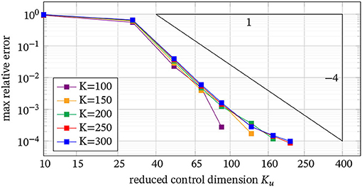
Figure 5. Max error for control dimensions of size K_u < K.

5.2.2. Combination With BT/RBM Error Decay

Next, we wish to investigate if a combination of a system theoretic MOR (here BT) and an RBM-like reduction with respect to time can be combined. To this end, we fix the temporal resolution (i.e., the number of time steps, here K = K_u = 300) and determine the RBM error using Algorithm 1 for the full and the BT-reduced system. We use [28] to compute the BT from [30] and obtain an LTI system of dimension $\widehat{n}=5$.

The results are shown in Figure 6, where we again show the maximal training error. As can be seen, the error for the BT-reduced system is smaller than the original one⁷, which in fact indicates that we can combine both methods. We get similar results for other choices of K. This shows that there is as much reduction potential in the reduced system eq. (5.2a) as in the original system eq. (5.1a). In other words, a combination of BT and RBM shows significant compression potential.

FIGURE 6

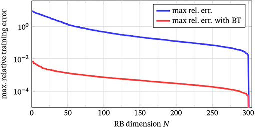
Figure 6. Maximal RBM relative error decay over the reduced dimension N for the full system eq. (5.1a) (blue) and the reduced system eq. (5.2a) with K = 300 (red).

However, applying BT first implies that the error estimator measures the difference with respect to the BT-reduced model and not with respect to the original problem, which means that we somehow lose part of the rigor implied by the fact that our error estimator coincides with the error. If one wants to preserve the rigor, it seems that a full pPDE model is required, which is possible in cases where the pDAE originates from a (known) discretization of a pPDE.

6. Conclusion and Outlook

In this article, we introduced a well-posed ultraweak formulation for DAEs and an optimally stable Petrov-Galerkin discretization, which admits a sharp error bound. The scheme shows the expected order of convergence depending on the regularity of the solution and the smoothness of the trial functions. The scheme also converges in low-regularity cases, where classical standard time-stepping schemes fail. Moreover, the stability of the Petrov-Galerkin scheme allows us to choose any temporal discretization without satisfying other stability criteria like a CFL condition.

Based upon the ultraweak framework, we introduced a model order reduction in terms of the Reduced Basis Method with an error/residual identity. We have obtained fast convergence and the possibility to combine the RBM for a reduction with respect to time with system theoretic methods such as Balanced Truncation to reduce the size of the system.

There are several open issues for future research. We already mentioned a primal-dual RBM for an efficient reduction of the output, the generalization to parameter-dependent matrices A_μ, and more general DAEs (not only fully linear). We also mentioned that the system matrix is a sum of Kronecker products of high dimension, which calls for specific solvers as in [21] for the (parameterized) wave equation. Another issue in that direction is the need for a basis of ker(E^T), which might be an issue for high-dimensional problems.

Data Availability Statement

The original contributions presented in the study are included in the article/supplementary material, further inquiries can be directed to the corresponding author/s.

Author Contributions

All authors listed have made a substantial, direct, and intellectual contribution to the work and approved it for publication.

Conflict of Interest

The authors declare that the research was conducted in the absence of any commercial or financial relationships that could be construed as a potential conflict of interest.

Publisher's Note

All claims expressed in this article are solely those of the authors and do not necessarily represent those of their affiliated organizations, or those of the publisher, the editors and the reviewers. Any product that may be evaluated in this article, or claim that may be made by its manufacturer, is not guaranteed or endorsed by the publisher.

Acknowledgments

We acknowledge support by the state of Baden-Württemberg through bwHPC.

Footnotes

1. ^Each regular matrix pencil can be transformed into Weierstrass-Kronecker canonical form P(λE − A)Q = diag(λId − W, λN − Id) with regular matrices P, Q ∈ ℂ^{n × n}, [15]. The index of a regular matrix pencil {E, − A} is then defined by ind{E, − A}: = ind{N}: = min{k ∈ ℕ : N^k = 0}.

2. ^By classical we mean defined in a pointwise manner.

3. ^The framework in [19] is slightly more general.

4. ^$Y_{\mu }^{\prime }$ denotes the dual space of Y_μ with respect to the pivot space L₂(Ω).

5. ^This is in fact the reason why we restricted ourselves to parameter-independent matrices E instead of E_μ. We would then need to have a parameter-dependent basis for $ker{E}_{\mu }^T$, which is, of course, possible, but causes a quite heavy notation.

6. ^For all quantities of the reduced system, we write the parameter μ as an argument in order to clearly distinguish the detailed approximation $x_{\mu }^{{N}}$ from the reduced approximation x_N(μ) for the same parameter.

7. ^This remains true even after additionally normalizing the training error by the dimensions of the DAE (n and $\widehat{n}$, respectively) or the dimension of the resulting linear system (Kn + d and $K\widehat{n}$, respectively).

References

1. Brenan KE, Campbell SL, Petzold LR. Numerical Solution of Initial-Value Problems in Differential-Algebraic Equations. Philadelphia, PA: SIAM (1995). doi: 10.1137/1.9781611971224

CrossRef Full Text | Google Scholar

2. Hairer E, Wanner G. Solving Ordinary Differential Equations II. Vol. 14. Berlin: Springer (2010).

Google Scholar

3. Kunkel P, Mehrmann V. Differential-Algebraic Equations. Zürich: European Mathematical Society (EMS) (2006).

Google Scholar

4. Trenn S. In: Ilchmann A, Reis T. Solution Concepts for Linear DAEs: A Survey. Berlin: Springer (2013). doi: 10.1007/978-3-642-34928-7_4

CrossRef Full Text | Google Scholar

5. Grundel S, Reis T, Schöps S. Progress in Differential-Algebraic Equations II. Cham: Springer (2020).

Google Scholar

6. Schöps S, Bartel A, Günther M, ter Maten EJ, Müller PC. Progress in Differential-Algebraic Equations. Berlin: Springer (2014).

Google Scholar

7. Benner P, Cohen A, Ohlberger M, Willcox K. Model Reduction and Approximation: Theory and Algorithms. Philadelphia, PA: SIAM (2017). doi: 10.1137/1.9781611974829

CrossRef Full Text | Google Scholar

8. Benner P, Stykel T. Model order reduction for differential-algebraic equations: A survey. In: Ilchmann A, Reis T, editors. Surveys in Differential-Algebraic Equations IV. Cham: Springer (2017). p. 107–60. doi: 10.1007/978-3-319-46618-7_3

CrossRef Full Text | Google Scholar

9. Chellappa S, Feng L, Benner P. Adaptive basis construction and improved error estimation for parametric nonlinear dynamical systems. Int J Num Methods Eng. (2020) 121:5320–49. doi: 10.1002/nme.6462

CrossRef Full Text | Google Scholar

10. Mehrmann V, Stykel T. Balanced truncation model reduction for large-scale systems in descriptor form. In: Benner P, Sorensen DC, Mehrmann V, editors. Dimension Reduction of Large-Scale Systems. Berlin: Springer (2005). p. 83–115. doi: 10.1007/3-540-27909-1_3

CrossRef Full Text | Google Scholar

11. Stykel T. Balanced truncation model reduction for descriptor systems. PAMM. (2003) 3:5–8. doi: 10.1002/pamm.200310302

CrossRef Full Text | Google Scholar

12. Stykel T. Gramian-based model reduction for descriptor systems. Math Control Signals Syst. (2004) 16:297–319. doi: 10.1007/s00498-004-0141-4

CrossRef Full Text | Google Scholar

13. Feuerle M, Urban K. A variational formulation for LTI-systems and model reduction. In: Vermolen FJ, Vuik C, editors. Numerical Mathematics and Advanced Applications ENUMATH 2019. Cham: Springer (2021). p. 1059–67. doi: 10.1007/978-3-030-55874-1_105

CrossRef Full Text | Google Scholar

14. Gear CW, Petzold LR. Differential/algebraic systems and matrix pencils. In: Kragström B, Ruhe A, editors. Matrix Pencils. Berlin: Springer (1983). p. 75–89. doi: 10.1007/BFb0062095

CrossRef Full Text | Google Scholar

15. Gantmacher FR. Theory of Matrices II. Providence, RI: Chelsea Publication (1959).

16. Hesthaven JS, Rozza G, Stamm B. Certified Reduced Basis Methods for Parametrized Partial Differential Equations. Cham: Springer (2016). doi: 10.1007/978-3-319-22470-1

CrossRef Full Text | Google Scholar

17. Barrault M, Maday Y, Nguyen NC, Patera AT. An empirical interpolation method: application to efficient reduced-basis discretization of partial differential equations. C R Acad Sci. (2004) 339:667–72. doi: 10.1016/j.crma.2004.08.006

CrossRef Full Text | Google Scholar

18. Chaturantabut S, Sorensen D. Nonlinear model reduction via discrete empirical interpolation. SIAM J Sci Comput. (2010) 32:2737–64. doi: 10.1137/090766498

CrossRef Full Text | Google Scholar

19. Dahmen W, Huang C, Schwab C, Welper G. Adaptive Petrov-Galerkin methods for first order transport equations. SIAM J Num Anal. (2012) 50:2420–45. doi: 10.1137/110823158

CrossRef Full Text | Google Scholar

20. Brunken J, Smetana K, Urban K. (Parametrized) First order transport equations: realization of optimally stable Petrov-Galerkin methods. SIAM J Sci Comput. (2019) 41:A592–621. doi: 10.1137/18M1176269

CrossRef Full Text

21. Henning J, Palitta D, Simoncini V, Urban K. An ultraweak space-time variational formulation for the wave equation: Analysis and efficient numerical solution. ESAIM: Math Modell Numer Anal. (2022) 56:1173–98. Available online at: https://www.esaim-m2an.org/articles/m2an/pdf/2022/04/m2an210138.pdf

Google Scholar

22. Urban K. The Reduced Basis Method in Space and Time: Challenges, Limits and Perspectives. Ulm: Ulm University (2022).

23. Arendt W, Urban K. Partial Differential Equations: An analytic and Numerical Approach. Transl. by J. B. Kennedy. New York, NY: Springer (2022).

24. Xu J, Zikatanov L. Some observations on Babuška and Brezzi theories. Num Math. (2003) 94:195–202. doi: 10.1007/s002110100308

CrossRef Full Text | Google Scholar

25. Henning J, Palitta D, Simoncini V, Urban K. Matrix oriented reduction of space-time Petrov-Galerkin variational problems. In: Vermolen FJ, Vuik C, editors. Numerical Mathematics and Advanced Applications ENUMATH 2019. Cham: Springer (2019). p. 1049–57. doi: 10.1007/978-3-030-55874-1_104

CrossRef Full Text | Google Scholar

26. Quarteroni A, Manzoni A, Negri F. Reduced Basis Methods for Partial Differential Equations: An Introduction. vol. 92. Springer (2015). doi: 10.1007/978-3-319-15431-2

CrossRef Full Text | Google Scholar

27. The The MathWorks Inc. MATLAB Version 9.11.0. Natick, MA (2021).

28. Saak J, Köhler M, Benner P. MM.ESS-2.2-The Matrix Equations Sparse Solvers Library. (2022). Available online at: https://www.mpi-magdeburg.mpg.de/projects/mess

Google Scholar

29. Schmidt M. Systematic Discretization of Input/Output Maps and Other Contributions to the Control of Distributed Parameter Systems. Berlin: TU Berlin (2007).

Google Scholar

30. Stykel T. Balanced truncation model reduction for semidiscretized Stokes equation. Linear Algebra Appl. (2006) 415:262–289. doi: 10.1016/j.laa.2004.01.015

CrossRef Full Text | Google Scholar

31. The The MORwiki Community. Stokes Equation. Magdeburg: MORwiki-Model Order (2018).

Google Scholar