Optimal statistical design of the double sampling np chart based on expected median run length

Introduction

Control chart is one of the most useful tools in Statistical Process Control since control charts play a key role in detecting the assignable cause(s) [1]. Other effective way to mitigate the incidence of false alarm rate and to increase the control chart sensitivity includes the fuzzy logic scheme [2–6], which combines the probability and fuzzy set theories for enabling inference of process state based on fuzzified sensitivity criteria. When the quality characteristics can only be classified into two possible outcomes, for instance, “Yes or No,” “Good or Bad,” “Conforming or Nonconforming,” and “Defective or Non-defective,” it is not possible to monitor the process using the variable control charts, such as the $\bar{X}$, s, and R charts. In such a scenario, attribute control charts will be the right choice.

The standard np chart is one of the attribute control charts that has been widely used for process monitoring. Compared to the p chart, the standard np chart is also easier to understand by managers who are lack of statistical knowledge and new to the quality control system. This provides more persuasive evidence of quality issues to management [7]. However, the standard np chart is well known to be slow in detecting moderate and small process fraction nonconforming (p) shifts. Consequently, considerable attentions have been devoted to develop np chart with various approaches for enhancing the sensitivity of the standard np chart in the literature, such as the optimal design for the cumulative sum (CUSUM) np chart by Gan [8] and the modified exponentially weighted moving average (EWMA) np chart by Gan [9]. Adaptive technique to develop np control chart has also been studied. Case in point, Epprecht and Costa [10] investigated the np properties for sample size that fluctuates between small and large sizes, while Luo and Wu [11] proposed optimal designs of variable sample size and variable sampling intervals np charts under steady-state mode.

Croasdale [12] was the first to introduce the DS scheme, bringing the concept of DS process from the acceptance sampling field and applying the technique to the $\bar{X}$ chart. Following Croasdale [12], Daudin [13] demonstrated that by employing the sample size of n₁ at stage 1 and combining two samples of size n₁ and n₂ at stage 2 can improve the performance of the $\bar{X}$ chart and this reduces the number of items to be inspected, resulting in a cost-saving benefit in the manufacturing process. As a result, the DS scheme developed after 1992, such as He and Grigoryan [14], Costa and Claro [15], Torng and Lee [16], Khoo et al. [17], and De Araujo Rodrigues et al. [18], to name a few, were based on the method proposed by Daudin [13]. De Araujo Rodrigues et al. [18] were the first to introduce the DS np chart. Chong et al. [19], Joekes et al. [20], Lee and Khoo [21], and Tuh et al. [22] have since focused their studies around the proposed DS np chart.

The performance of the control charts is usually evaluated by the average run length (ARL). ARL is defined as the average number of samples to be plotted on the control chart before the out-of-control signal is observed. However, many researchers criticized the sole dependence of the ARL as the performance measure of control charts, for example, see Teoh et al. [23], Khoo et al. [24], Lee and Khoo [25], Smajdorová and Noskievičová [26]. In addition, as pointed out by Graham et al. [27], the ARL as a performance measure has many drawbacks. It is noted that the run length (RL) distribution is changing from highly right-skewed when process shift size is small to almost symmetric when process shift size is large. Consequently, utilizing the ARL as a performance measure may neglect some vital statistical properties of control charts. Chakraborti [28] recommended to investigate the percentiles of the run length distribution such as 5, 25, 50 (median), 75, and 95th percentiles to have a better vision and evaluation of the RL distribution. Utilizing the median run length (MRL) that is the 50th percentile of the RL has some additional benefits in designing control charts [29–31]. This is due to the fact that the MRL is less impacted by the skewness of the RL distribution. Thus, the MRL provides a more accurate measure of the central tendency compared to the ARL [32].

Existing work on the DS np control chart based on MRL by Tuh et al. [22] assumes the shift size is known. However, the shift size of the process fraction nonconforming is usually unknown by quality practitioners. The performance of control charts may be negatively impacted if the determined shift size differs from the actual value. To overcome this issue, it is crucial to consider the expected median run length (EMRL) as an alternative performance measure, where only a range of process shift sizes is required. You et al. [33], Teoh et al. [34], Tang et al. [35], Chong et al. [36], and Yeong et al. [37], to name a few, evaluated the performance of control charts when the process shift size is unknown. Motivated by these studies, we suggest the optimal design of the DS np chart based on EMRL in this paper.

The paper is structured as follows: Section Theories and formulations begins with a brief introduction of the standard np and DS np charts, followed by a discussion of the RL distribution properties of the DS np chart. Section Computational methods and results presents the optimization design of the EMRL-based DS np chart, performance of the DS np chart, and comparison to that of the standard np chart. The operability of the DS np chart is also furnished through an illustrative example incorporating event within a data processing department. Finally, the conclusion is given in section Conclusions.

Theories and formulations

The standard np chart

The goal of the standard np chart is to detect the assignable causes for increasing shift in the process fraction nonconforming. As a result, the standard np chart is designed without a lower control limit. According to Lee and Khoo [29], the probability that d < UCL is calculated as follows:

$\begin{array}{ll}{A}_S=P(d\le \lfloor UCL\rfloor )={\displaystyle \sum _{d=0}^{\lfloor UCL\rfloor }}\frac{n!}{d!(n-d)!}{p}^d{(1-p)}^{n-d}& (1)\end{array}$

where p = p₀ when γ = 1, and p = p₁ when γ ≠ 1. The d and UCL represent the number of nonconforming items found in a sample of size n and upper control limit of the standard np chart, respectively.

The DS np chart

In this section, we give a brief review of the DS np chart, which was first introduced by De Araujo Rodrigues [18]. To achieve the desired statistical performance, the DS np chart is designed with five charting parameters. We define the set of charting parameters as n₁, n₂, WL, CL₁, and CL₂, where n₁, n₂, WL, CL₁, and CL₂ denote the size of the first sample, the size of second sample, the stage 1 warning limit, the stage 1 control limit, and the stage 2 control limit, respectively. The three non-integer control limits are set as WL = Ac₁ + 0.5, CL₁ = Re – 0.5, and CL₂ = Ac₂ + 0.5 to avoid doubt by quality practitioners when the number of nonconforming items in a sample falls within or outside the control limits. In these expressions, Ac₁, Re₁, and Ac₂ are the acceptance number in the first sample, the rejection number in the first sample, and the acceptance number in the stage 2, respectively. The operation of the DS np chart is elaborated in the following steps. The graphical summary is shown in Figure 1.

Step 1. Determine the limits that are WL, CL₁, and CL₂.

Step 2. Take the first sample of size n₁ from the process and check the number of nonconforming items (d₁).

Step 3. At the stage 1 of the DS scheme,

a) if d₁ < WL, the process is considered as in-control and return to Step 2.

b) if d₁ > CL₁, the process is considered as out-of-control. For the purpose of identifying and eliminating the assignable cause(s), corrective measure is performed. Repeat Step 2.

c) if WL < d₁ < CL₁, take a second sample with size n₂. Count the number of nonconforming items (d₂) for the second sample. Then, move to the next step, which is stage 2 of the DS scheme.

Step 4. If (d₁ + d₂) < CL₂, the process is considered to be in-control and return to Step 2. Else, the process is deemed to be out-of-control. To locate and remove the assignable cause(s), corrective action is once again performed. Repeat Step 2.

FIGURE 1

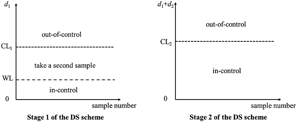
Figure 1. Regions at stages 1 and 2 of the DS schemes.

The run length properties of the DS np chart

In general, RL denotes the number of sample points plotted on the DS np chart before the first signal is observed. The probability mass function (pmf) f_RL(ζ) and the cumulative distribution function (cdf) F_RL(ζ) of the RL distribution for a control chart are

$\begin{array}{ll}{f}_{RL}(\zeta )=(1-A)A^{\zeta -1}& (2)\end{array}$

and

$\begin{array}{ll}{F}_{RL}(\zeta )=P(RL\le \zeta )=1-A^{\zeta },& (3)\end{array}$

respectively [38], where ζ ∈ {1, 2, 3, 4, …} and A is calculated by Equations (5) and (6).

As suggested by Chakraborti [28], the smallest integer of the percentile run length, ζ_α, can be obtained from

$\begin{array}{ll}{\zeta }_{\alpha }\ge \frac{ln(1-\alpha )}{lnA}& (4)\end{array}$

facilitates the computation for the 100αth (0 < α < 1) percentile of the RL.

The probability that the process is in-control is given by A = A₁ + A₂. Here, A₁ denotes the probability that d₁ < WL at the stage 1 of the DS scheme, while A₂ is the probability that WL < d₁ < CL₁ at the stage 1 of the DS scheme and (d₁ + d₂) < CL₂ at the stage 2 of the DS scheme, where

$\begin{array}{ll}{A}_1=P(d_1\le \lfloor WL\rfloor )={\displaystyle \sum _{d_1=0}^{\lfloor WL\rfloor }}\frac{n_1!}{d_1!(n_1-d_1)!}{p}^{d_1}{(1-p)}^{n_1-d_1}& (5)\end{array}$

and

$\begin{array}{ll}{A}_2=P({\lfloor WL\rfloor <d}_1<\lceil C{L}_1\rceil )\cap P(d_1+d_2\le \lfloor C{L}_2\rfloor )={\displaystyle \sum _{d_1=\lfloor WL\rfloor +1}^{\lceil C{L}_1\rceil -1}}\left[\frac{n_1!}{d_1!(n_1-d_1)!}{p}^{d_1}{(1-p)}^{n_1-d_1}\left({\displaystyle \sum _{d_2=0}^{\lfloor C{L}_2\rfloor -d_1}}\frac{n_2!}{d_2!(n_2-d_2)!}{p}^{d_2}{(1-p)}^{n_2-d_2}\right)\right],& (6)\end{array}$

where ⌊ · ⌋ denotes the round down to the nearest integer and ⌈ · ⌉ represents the round up to the nearest integer.

The efficiency of the DS np chart is determined by how fast the chart can detect an increasing shift in the process fraction nonconforming p with the shift size $\gamma =\frac{p_1}{p_0}$, where p₁ > p₀. Note that p = p₀ and p = p₁ for the in-control (γ = 1) and out-of-control (γ > 1) states, respectively. According to De Araujo Rodrigues et al. [18], the ARL and the average sample size (ASS) can be computed as

$\begin{array}{ll}ARL=\frac{1}{1-A}and& (7)\end{array}$

$\begin{array}{ll}ASS=n_1+n_2{P}_s,& (8)\end{array}$

respectively, where P_s = P(⌊WL⌋ < d₁ < ⌈CL₁⌉). The in-control ARL (ARL₀) and ASS (ASS₀) are calculated when p = p₀, while the out-of-control ARL (ARL₁) and ASS (ASS₁) can be obtained when p = p₁.

The MRL is the RL with a cumulative probability of at least 50% of the time. The MRL can be computed using Equation (4) by putting α = 0.5, where Equation (4) can be rewritten as

$\begin{array}{ll}{\zeta }_{0.5}\ge \frac{ln(0.5)}{lnA},& (9)\end{array}$

where ζ_0.5 = MRL. Note that MRL = MRL₀ is the in-control MRL when γ = 1, whereas MRL = MRL₁ is the out-of-control MRL when γ > 1.

The computation of the percentiles of the RL requires the shift size to be known in advance. However, in practical, it is usually tough for practitioners to quantify the magnitude of process shift due to insufficient historical data. Aside from that, the shift size varies according to various undetermined or random events [39]. Thus, the percentile of the RL can be replaced by the expected percentile of the RL (E(ζ_α)). Herein, a specific value for γ is not required and can be determined as follows:

$\begin{array}{ll}E({\zeta }_{\alpha })={\displaystyle {\int }_{{\gamma }_{min}}^{{\gamma }_{max}}}{f}_{\gamma }(\gamma ){\zeta }_{\alpha }(\gamma )d\gamma .& (10)\end{array}$

Hence, the expected median run length, EMRL, that is E(ζ_0.5) can be computed as

$\begin{array}{ll}EMRL=E({\zeta }_{0.5})={\displaystyle {\int }_{{\gamma }_{min}}^{{\gamma }_{max}}}{f}_{\gamma }(\gamma )MRL(\gamma )d\gamma .& (11)\end{array}$

In this paper, the EMRL in Equation (11) is evaluated by using a numerical integration over the probability density function f_γ(γ) for a shift size interval of γ_min (the lower limit of the integral) to γ_max (the upper limit of the integral). The function f_γ(γ) is assumed to have a continuous uniform distribution over the interval (γ_min, γ_max) [39], with probability density function of $f_{\gamma }(\gamma )=\frac{1}{({\gamma }_{max}-{\gamma }_{min})}$, where γ_max − γ_min denotes the interval length. To incorporate exact shift sizes, γ ∈ {1.5, 2.0, 3.0}, that were considered in Tuh et al. [22], two intervals of the shift size, therefore, are set in this paper: (i) (γ_min , γ_max] = (1.1 , 2.0] and (ii) (γ_min , γ_max] = (2.0 , 3.0]. For example, the interval (γ_min , γ_max] = (1.1 , 2.0] and (γ_min , γ_max] = (2.0 , 3.0] include γ = {1.5, 2.0} and γ = {3.0}, respectively. Note that MRL(γ) denotes the MRL₁ at γ. The Gauss Legendre Quadrature is employed to estimate approximately the definite integral in Equation (11).

This paper also evaluates the expected average run length (EARL) and the expected average sample size (EASS) values through

$\begin{array}{ll}EARL={\displaystyle {\int }_{{\gamma }_{min}}^{{\gamma }_{max}}}{f}_{\gamma }(\gamma )ARL(\gamma )d\gamma & (12)\end{array}$

and

$\begin{array}{ll}EASS={\displaystyle {\int }_{{\gamma }_{min}}^{{\gamma }_{max}}}{f}_{\gamma }(\gamma )ASS(\gamma )d\gamma ,& (13)\end{array}$

respectively.

Computational methods and results

Optimal design of the EMRL-based DS np chart

Tuh et al. [22] investigated the performance of the DS np chart using the MRL as the performance measure. Interested readers may refer to Tuh et al. [22] for the detailed optimization procedure for the DS np chart based on the MRL.

Nevertheless, the actual process shift size is usually unknown. Thus, the DS np chart can be designed for a given range of shift sizes (γ_min, γ_max], which is an alternative method. The optimization design of the DS np chart by minimizing the out-of-control expected median run length (EMRL₁) is given as

$\begin{array}{ll}{min}_{n1,n2,WL,CL1,CL2}EMR{L}_1& (14)\end{array}$

subject to:

$\begin{array}{ll}EMR{L}_0\ge MR{L}_{0min}and& (15)\end{array}$

$\begin{array}{ll}EAS{S}_0=n.& (16)\end{array}$

MRL_0min [in Constraint (15)] and n [in Constraint (16)] are denoted as the predetermined in-control median run length and predetermined in-control average sample size, respectively, where n₁ < n < n₂, with both n₁ and n₂ are integers. Note that EMRL₀ = MRL₀ and EASS₀ = ASS₀ are considered in this paper.

The procedure for searching optimal (n₁, n₂, WL, CL₁, CL₂) combination, based on the optimization model in (14)–(16), and the DS np chart based on EMRL is outlined as follows:

Step 1: Specify the desired values of p₀, n, MRL_0min, γ_min, and γ_max. Here, n is the average sample size in each sampling when the process is in a state of control; n is also the fixed sample size for the standard np chart.

Step 2: Initialize EMRL_1min with a very large value, say 10⁵. EMRL_1min is used to keep track of the lowest EMRL₁ value.

Step 3: Begin with n₁ = 1.

Step 4: With the current n₁ value, determine the combination of (n₁, n₂, WL, CL₁) for a specified n when γ = 1, such that the Constraint (16) is fulfilled. The value of n₂ is computed through the rearrangement of Equation (8), that is, $n_2{=}^{(n-n_1)}{/}_{\mathrm{\text{P}}(\lfloor \mathrm{\text{WL}}\rfloor <d_1<\lceil \mathrm{\text{C}}{\mathrm{\text{L}}}_1\rceil )}$, and is rounded up to the nearest integer, where 0 < WL < CL₁.

Step 5: Then determine CL₂ based on the Equation (9) and Constraint (15), in which the computed EMRL equals to EMRL₀ when γ = 1, where CL₂ > CL₁. The values of WL, CL₁, and CL₂ are determined based on operating procedure discussed in Section 2.2. In this step, the possible (n₁, n₂, WL, CL₁, CL₂) combination is identified.

Step 6: Once the possible (n₁, n₂, WL, CL₁, CL₂) combination has been determined, EMRL₁ will be computed for p = p₁, by means of Equation (11). If the calculated EMRL₁ is less than the current EMRL_1min, the EMRL_1min value will be replaced by the newly computed EMRL₁. The current (n₁, n₂, WL, CL₁, CL₂) combination is temporarily stored as the possible combination before any new lower EMRL₁ value is found. If the (n₁, n₂, WL, CL₁, CL₂) combination obtained in the following search yields similar EMRL_1min, the combination will be saved together as a possible combination. Otherwise, the (n₁, n₂, WL, CL₁, CL₂) combination will not be considered if it results in larger EMRL₁ value.

Step 7: Once the search with n₁ = 1 is complete, increase n₁ by one. Repeat Steps 4–6, for the remaining n₁ = 2, 3…, (n − 1), to search for the possible (n₁, n₂, WL, CL₁, CL₂) combinations that satisfy the Constraints (15)–(16) and having the smallest value of EMRL₁.

Step 8: If more than one combinations of (n₁, n₂, WL, CL₁, CL₂) produce a similar lowest EMRL₁ value, the combination that yields the smallest out-of-control expected average sample size (EASS₁) value is selected as the optimal combination.

An optimization MATLAB program is developed to execute the above procedure to search for the optimal (n₁, n₂, WL, CL₁, CL₂) combination for the EMRL-based DS np chart.

In this paper, based on the Gauss Legendre Quadrature rule, the weights (w_i) and nodes (x_i) values are obtainable through the MATLAB coding written by Winckel [40]. These values are considered for the computation of E(ζ_α)₁, EARL₁, and EASS₁. According to Hale and Townsend [41], the fundamental accuracy can be achieved for any number of ordinates (N) that exceeds 100. Therefore, N = 200 is considered for all these computations.

Comparative studies

In this section, the EMRL₁ performance of the standard np chart with unknown shift size is compared with that of the DS np chart. The computational procedure for the standard np chart based on the EMRL₁ is to find the minimal value of UCL given the sample size n, by attaining the constraint EMRL₀ ≥ MRL_0min. The E(ζ_0.5)₀ (= MRL₀) and EARL₀ (= ARL₀) of the standard np chart are computed using Equations (9) and (7), respectively, by replacing A with A_S from Equation (1). The optimal charting parameters of the DS np chart are computed using the optimization procedure described in Section Optimal design of the EMRL-based DS np chart. The different combinations of input parameters as follows are considered: p₀ ∈ {0.005, 0.01, 0.02}, MRL_0min ∈ {200, 370.4}, n ∈ {25, 50, 100, 200, 400, 800}, and two intervals of process shift sizes: (1) (γ_min, γ_max] = (1.1, 2.0] and (2) (γ_min , γ_max] = (2.0 , 3.0]. We only provide the results for the combinations of n and p₀ such that np₀ = {0.5, 1.0, 2.0, 4.0}. The and p₀ combinations that generate np₀ = {0.5, 1.0, 2.0, 4.0} were also adopted by several researchers [see [10], [29], and [19]] for clarity and unbiased comparison between competing charts.

Performance of the standard np and DS np charts based on EMRL

The charting parameter UCL for the standard np and the optimal charting parameters (n₁, n₂, WL, CL₁, CL₂) of the DS np chart based on the EMRL₁ are listed in Tables 1, 2. The corresponding values of E(ζ_0.05)₀, EMRL₀, E(ζ_0.95)₀, and EARL₀ are also provided in the tables. Note that E(ζ_0.05)₀ and E(ζ_0.95)₀ denote the in-control 5th and 95th percentiles of the RL, respectively. For example, Table 2 shows that when p₀ = 0.01, n = 100 and (γ_min, γ_max] = (1.1, 2.0], for the standard np chart, while (n₁, n₂, WL, CL₁, CL₂) = (27, 2454, 1.5, 4.5, 34.5) for the optimal DS np chart. The DS np chart with these charting parameters gives the smallest EMRL₁ value, while the EMRL₀ is at least 370.4. Subsequently, the corresponding values of (E(ζ_0.05)₀, EMRL₀, E(ζ_0.95)₀, EARL₀) for the standard np and optimal DS np charts are computed as (96, 1,297, 5,603, 1,870.79) and (29, 385, 1,661, 554.77), respectively. The optimal design makes the DS np chart easier to implement in practice. Consider the case of a plastic component created via injection molding, for which a rapid detection within the range of process shift sizes (γ_min, γ_max] = (1.1, 2.0] is required. Table 1 suggests (n₁, n₂, WL, CL₁, CL₂) = (24, 1,090, 1.5, 4.5, 16.5) as the best charting parameter for detecting this range of shift sizes if p₀ = 0.01, n = 50, and MRL_0min = 200.

TABLE 1

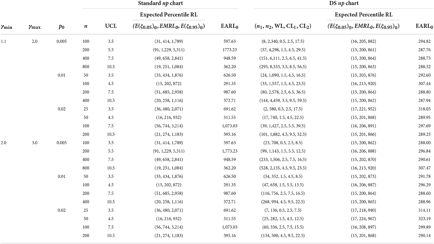
Table 1. Charting parameters with corresponding (E(ζ_0.05)₀, EMRL₀, E(ζ_0.95)₀) and EARL₀ for standard np and optimal DS np charts, when MRL_0min = 200.

TABLE 2

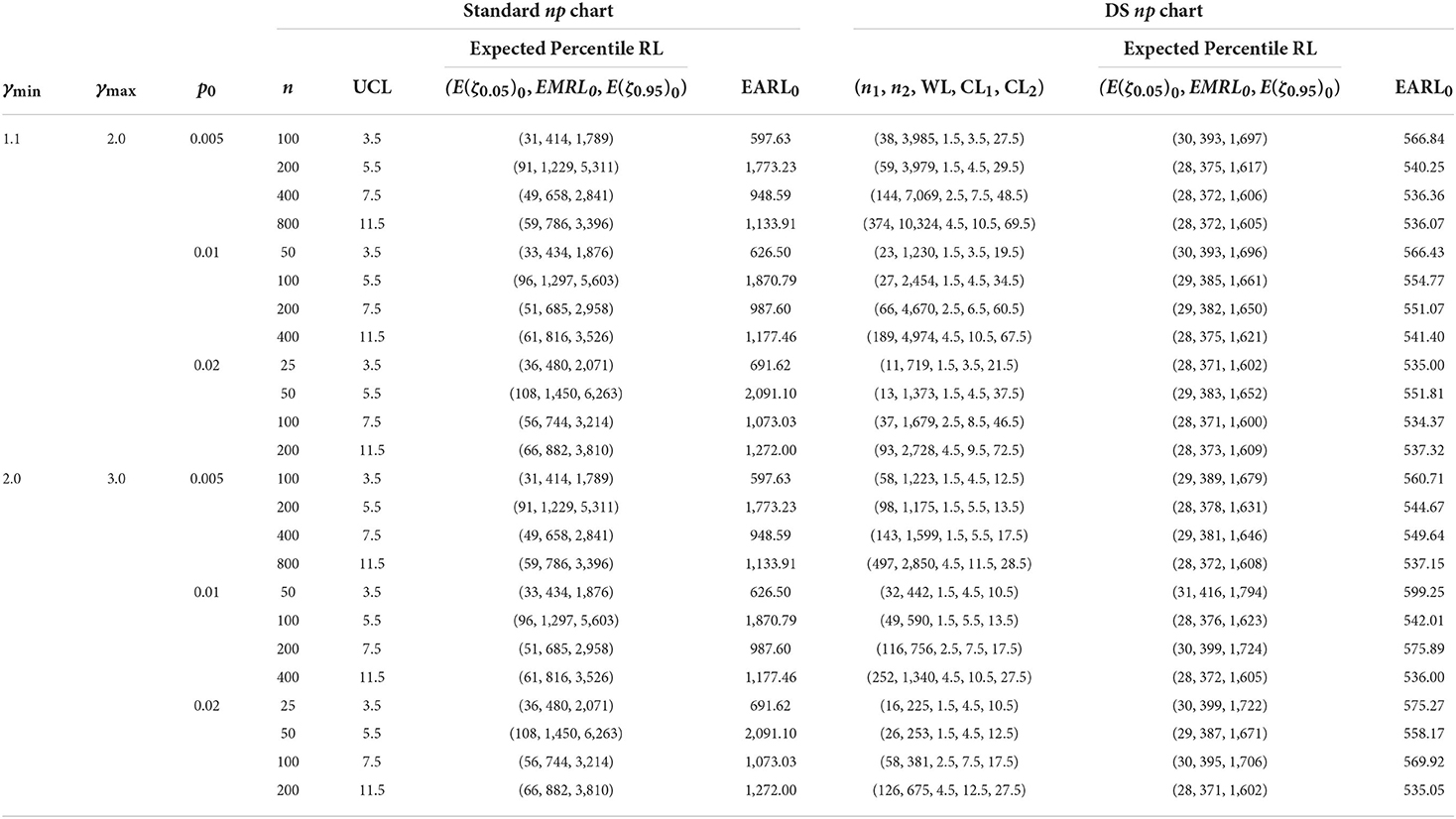
Table 2. Charting parameters with corresponding and EARL₀ for standard np and optimal DS np charts, when MRL_0min = 370.4.

In Table 3, the E(ζ_0.05)₁, EMRL₁, E(ζ_0.95)₁, and EARL₁ values, for the out-of-control case, can be obtained using the charting parameter UCL for the standard np and optimal charting parameters (n₁, n₂, WL, CL₁, CL₂) of the DS np charts (refer to Tables 1, 2). For instance, when p₀ = 0.02, n = 50, MRL_0min = 200, and (γ_min, γ_max] = (1.1, 2.0], Table 1 gives (n₁, n₂, WL, CL₁, CL₂) = (17, 740, 1.5, 4.5, 22.5) as the optimal charting parameters for the DS np chart. With these optimal charting parameters, (E(ζ_0.05)₁, EMRL₁, E(ζ_0.95)₁, EARL₁) = (1.83, 18.50, 78.34, 26.49). The equations used for the evaluation of E(ζ_0.05)₁, EMRL₁, E(ζ_0.95)₁, and EARL₁ values can be found in Section The run length properties of the DS np chart.

TABLE 3

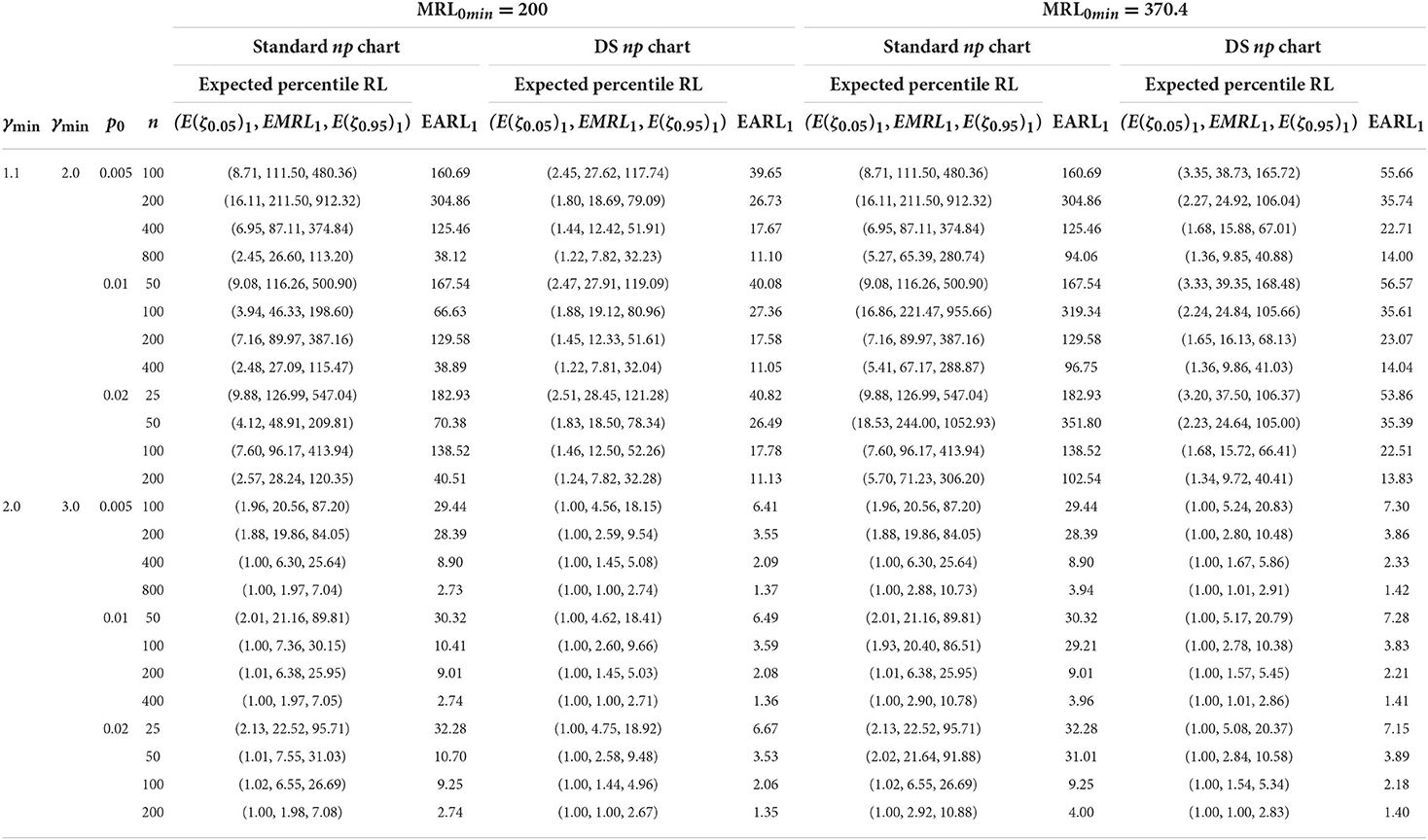
Table 3. Performance of the DS np and standard np charts with MRL_0min = 200 and 370.4.

Numerical results in Tables 1, 2 clearly demonstrate that the EMRL₀ values are lower than EARL₀, for both standard np and optimal DS np charts for the in-control case (γ = 1). For instance, referring to Table 1, the DS np chart gives EARL₀ = 314.11 when p₀ = 0.02, = 25, (γ_min , γ_max] = (2.0 , 3.0], and MRL_0min = 200. Practitioners may interpret a false alarm happens by the 314th sample in half of the time. In fact, this value is located in between 60 and 70th (= 378) percentile of the RL distribution, and the false alarm actually happens before 314th sample, that is by the 218th sample (EMRL₀ = 218), occurs in half of the time. On the contrary, for the out-of-control case (see Table 3), when p₀ = 0.02, n = 100, (γ_min , γ_max] = (2.0 , 3.0], and MRL_0min = 200, the DS np chart gives EARL₁ = 2.06, while EMRL₁ = 1.44, showing small difference between the EARL₁ and EMRL₁ values. This demonstrates that when the RL distribution is highly right-skewed, the average is significantly larger than the median. In contrast, the average is relatively closer to the median in symmetric distribution. Consequently, we recommend the EMRL over EARL as a performance measure which delivers a clearer interpretation for the performance DS np chart. In addition, based on the EMRL performance measure, Table 3 shows that the optimal DS np chart outperforms the standard np chart for all shift sizes, (γ_min, γ_max], with the former giving lower EMRL₁ than the latter for identical p₀, n, MRL_0min, and (γ_min, γ_max] combination.

Performance of the standard np and DS np charts based on expected percentile of the RL distribution

The percentiles of RL distribution can help to reveal more information about the entire RL distribution, including the early false alarm rates. In this paper, the E(ζ_0.05) and E(ζ_0.95) are also analyzed to equip practitioners with a better view on the spread of the entire RL distribution of the standard np and optimal DS np charts.

The lower percentile, such as E(ζ_0.05) evaluated in this paper for the in-control case (γ = 1), provides information concerning early false alarm rates. Let us consider standard np chart in Table 1, when p₀ = 0.01, n = 50, MRL_0min = 200, and (γ_min, γ_max] = (1.1, 2.0], gives E(ζ_0.05)₀ = 33. This result suggests a false alarm will occur by 33rd sample point in 5% of the time. On the contrary, a false alarm will happen in half of the time by the 434th sample (E(ζ_0.5)₀ = 434), meaning that sample 434 has a chance of 0.5 of detecting a false alarm, whereas the EARL₀ is indicated as 626.50.

On the other hand, the higher percentile of the RL distribution, for example, E(ζ_0.95)₁, provides information about the out-of-control condition which will be issued by the control chart with a high possibility at a certain magnitude of the shift. Based on DS np chart, as shown in Table 3, when p₀ = 0.005, MRL_0min = 370.4, n = 100, and (γ_min, γ_max] = (2.0, 3.0], this chart is anticipated to signal within the first 20.83 samples with a probability of 0.95 (E(ζ_0.95)₁ = 20.83). In other words, practitioners can claim with 95% confidence that an out-of-control signal will be discovered by the 20.83rd sample.

Moreover, both the standard np and DS np charts, shown in Tables 1, 2, clearly demonstrate that the in-control RL is subject to significant variation. Expectedly, in Table 2, the in-control extreme percentile of the DS np chart is 1,722 – 30 = 1,692 and the standard np chart is 2,071 – 36 = 2,035 when p₀ = 0.02, n = 25, (γ_min, γ_max] = (2.0, 3.0], and MRL_0min = 370.4.

However, by referring to Table 3 for the out-of-control condition, the extreme percentile (the difference between the E(ζ_0.05) and E(ζ_0.95)) reduces as n increases and the shifts interval changes from (γ_min, γ_max] = (1.1, 2.0] (small shifts interval) to (γ_min, γ_max] = (2.0, 3.0] (large shifts interval), for both standard np and DS np charts. This trend suggests that there is small variation for the out-of-control RL over large shift interval and larger n values. For example, the out-of-control extreme percentile of the DS np chart is 103.17 when MRL_0min = 370.4, p₀ = 0.02, n = 25, and (γ_min, γ_max] = (1.1, 2.0], diminishes to 19.37 when (γ_min, γ_max] = (2.0, 3.0], for identical p₀, n, and MRL_0min. In addition, the numerical results reveal that the optimal DS np chart has smaller variation in RL distribution compared to the competing standard np chart for small and large shift interval.

Performance of the DS np chart when shift size is unknown

The most interesting finding emerges from the analysis shown in Tables 4–6, utilizing the optimal parameters by minimizing EMRL₁ to compute the MRL₁ when unknown shift size is a viable option, providing γ ϵ (γ_min, γ_max]. The optimal charting parameters for the EMRL-based DS np chart can be obtained from Tables 1, 2. For ease of reference and comparison, the MRL₁ of MRL-based design chart found by Tuh et al. [22] is listed in Tables 4–6. For a comprehensive comparison, the MRL₁ values for both MRL-based and EMRL-based design charts when γ = 1.2 are also added to this section. Due to space constraint, we only present the results with n = 100.

TABLE 4

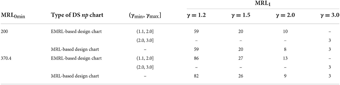
Table 4. MRL₁ computed using the optimal charting parameters of the EMRL-based DS np chart and the MRL-based DS np chart for p₀ = 0.005, n = 100, and EMRL₀ ∈ {200, 370.4}.

TABLE 5

Table 5. MRL₁ computed using the optimal charting parameters of the EMRL-based DS np chart and the MRL-based DS np chart for p₀ = 0.01, n = 100, and EMRL₀ ∈ 200, 370.4.

TABLE 6

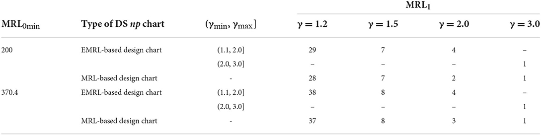
Table 6. MRL₁ computed using the optimal charting parameters of the EMRL-based DS np chart and the MRL-based DS np chart for p₀ = 0.02, n = 100, and EMRL₀ ∈ {200, 370.4}.

From Tables 4–6, it is worth noting that the MRL₁ computed in Tables 4–6 by means of (n₁, n₂, WL, CL₁, CL₂) for DS np chart with EMRL-based design is nearly identical to those based on specific shift sizes (MRL-based design chart) for most cases, on condition that γ ϵ (γ_min, γ_max]. For instance, in Table 5, when n = 100, MRL_0min = 200, p₀ = 0.02, and (γ_min, γ_max] = (1.1, 2.0], the optimal charting parameters of the DS np chart are (n₁, n₂, WL, CL₁, CL₂) = (39, 1,427, 2.5, 5.5, 39.5) (see Table 1), obtained by minimizing EMRL₁. This optimal charting parameters yield MRL₁ = {29, 7, 4} for γ = {1.2, 1.5, 2.0}, while the MRL-based design chart gives MRL₁ = {28, 7, 2}. As a result, the optimal parameters listed in Tables 1, 2 (as determined by minimizing EMRL₁) can be directly and reliably substituted for the optimal parameters by assuming a known shift size, in the event that γ ϵ (γ_min, γ_max].

An illustrative example

The performance of the DS np chart is assessed with the use of an example, as follows. The information used in this illustration was extracted from Gitlow and Hertz [42]. The information is relevant to the keypunching operation that normally takes place in a data processing department. To establish the control chart, a sample size of 200 cards (n = 200) was selected at random from the output of each day's production over the course of 24 days (subgroups m = 24) and inspected for defects. After establishing the control chart, it was discovered that samples 8 and 22 were not within the control limits and were subsequently discarded following further investigation. Using the remaining samples of m = 22 and n = 200, revised control limits were computed. All the verified points fall within the control limits, pointing toward in-control process. This represents phase I analysis. As a result, we may estimate the in-control process fraction nonconforming (p₀) using following equation:

$\begin{array}{ll}{p}_0=\frac{{\displaystyle {\sum }_{i=1}^m}{p}_i}{m}=\frac{{\displaystyle {\sum }_{i=1}^m}{d}_i}{m\times n}=\frac{73}{22\times 200}\approx 0.02& (17)\end{array}$

We illustrate the proposed optimal EMRL-based DS np chart by applying a simulated data generated using the RStudio software. Herein, we use the optimal charting parameters based on MRL_0min = 200, (γ_min, γ_max] = (1.1, 2.0], p₀ = 0.02, and n = 200 obtained from Table 1. The optimal parameter combination for the DS np chart is (n₁, n₂, WL, CL₁, CL₂) = (101, 1,882, 4.5, 9.5, 52.5). The data for the 30 samples are simulated, where the first eight samples come from the in-control state with p₀ = 0.02. The subsequent 22 samples depict the out-of-control state with p₁ = γp₀ = 1.3 × 0.02 = 0.026, where a process shift of γ = 1.3 is presumed to have occurred. Note that the number of nonconforming items in the first sample d₁ is simulated from the binomial distribution with parameters (n₁, p₀) = (101, 0.02) and (n₁, p₁) = (101, 0.026) for the in-control and out-of-control states, respectively, while the number of nonconforming items for the second sample d₂ is generated from the same distribution but with parameters (n₂, p₀) = (1,882, 0.02) and (n₂, p₁) = (1,882, 0.026) for the in-control and out-of-control cases, respectively.

The thirty samples from Table 7 are plotted in Figure 2's DS np chart. The solid dots (•) and hollow dots (◦) represent the stages 1 and 2 of the DS scheme, respectively. One can observe that the process remains at the stage 1 of the DS scheme for samples 1 through 6 as the points lie lower than 4.5 (<WL) and is deemed to be in-control. Note that at sample 7, d₁ = 5 for the first sample at the stage 1 of the DS scheme corresponds to size n₁ = 101. Since 4.5 < d₁ < 9.5, the operation moves to the stage 2 of the DS scheme, which involves taking a second sample of size n₂ = 1,882 and number of nonconforming items d₂ = 36 is observed. As a result, d₁ + d₂ = 5 + 36 = 41. Since d₁ + d₂ is below 52.5 (<CL₂), this sample is considered as in-control. The process remains in-control condition up to sample 14. At sample 15, d₁ = 6, d₂ = 54 in which d₁ + d₂ = 60 exceeds the control limit CL₂ of 52.5. This indicates that sample 15 is out-of-control. Clearly, DS np chart detects the process shift at sample 15. Corrective action should be taken immediately to identify and remove the assignable cause(s) that resulting to the out-of-control condition in the process.

TABLE 7

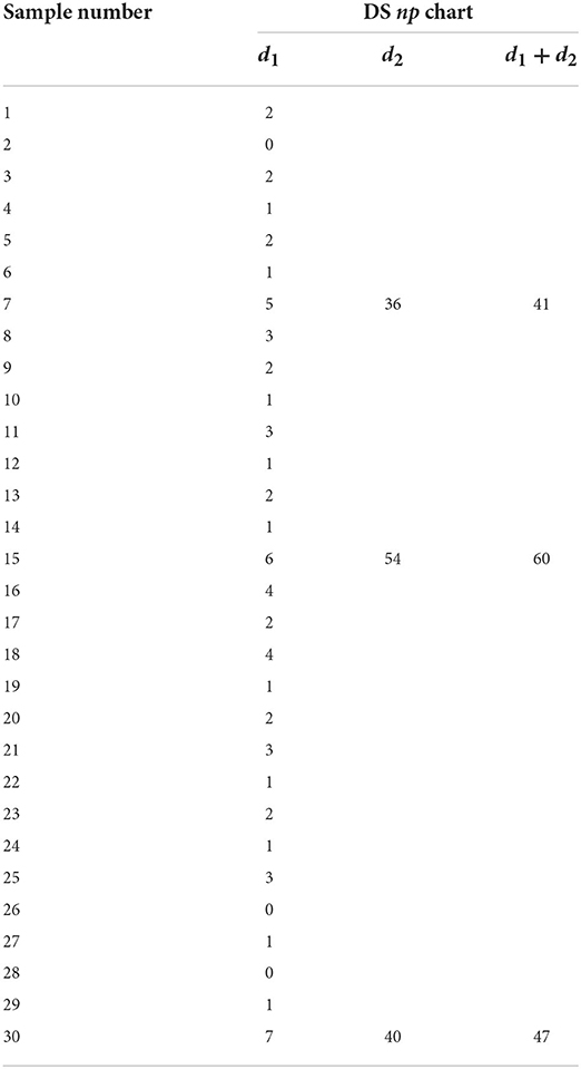
Table 7. Dataset for the illustrative example.

FIGURE 2

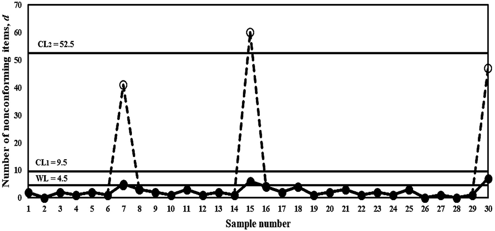
Figure 2. DS np chart.

Conclusion

A good understanding of a control chart is crucial as it helps to increase the confidence of quality practitioners. Therefore, in this study, EMRL has been proposed as a performance measure for designing DS np chart. The results obtained indicate that the EMRL is an effective optional performance measure for the DS np chart when it is not possible to specify the shift size of the fraction nonconforming beforehand. Alternatively, practitioners can utilize the recommended optimal charting parameters based on EMRL₁ minimization if the process shift size is within the acceptable range (γ_min, γ_max]. In the case of inexperienced practitioners who are not familiar with the establishment of process shift size, this approach can help to minimize inaccuracy that may arise when practicing and implementing the DS np control chart. It should be noted that the conclusion in this research depends on the data independence and binomially distributed assumptions. For future research purposes, additional work can be carried out without applying these assumptions. In addition, the effect of parameter estimation may also be conducted for the unknown shift size.

Data availability statement

The original contributions presented in the study are included in the article/supplementary material, further inquiries can be directed to the corresponding author/s.

Author contributions

MT: conceptualization, methodology, software, formal analysis, investigation, data curation, project administration, and writing—original draft. CK and HC: software, validation, resources, and writing—reviewing and editing. ML: validation, visualization, and writing—reviewing and editing. All authors contributed to the article and approved the submitted version.

Acknowledgments

We gratefully acknowledge Dr. Robin Chang Yee Hui for lending us his personal computing resources to carry out part of the calculations shown in this study.

Conflict of interest

The authors declare that the research was conducted in the absence of any commercial or financial relationships that could be construed as a potential conflict of interest.

Publisher's note

All claims expressed in this article are solely those of the authors and do not necessarily represent those of their affiliated organizations, or those of the publisher, the editors and the reviewers. Any product that may be evaluated in this article, or claim that may be made by its manufacturer, is not guaranteed or endorsed by the publisher.

References

1. Montgomery DC. Introduction to Statistical Quality Control. New York: John Wiley & Sons (2020).

2. Kumar PS. A simple method for solving type-2 and type-4 fuzzy transportation problems. Int J Fuzzy Logic Intell Syst. (2016) 16:225–37. doi: 10.5391/IJFIS.2016.16.4.225

CrossRef Full Text | Google Scholar

3. Kumar PS. Algorithms for solving the optimization problems using fuzzy and intuitionistic fuzzy set. Int J Syst Assur Eng Manage. (2020) 11:189–222. doi: 10.1007/s13198-019-00941-3

CrossRef Full Text | Google Scholar

4. Kumar PS. Intuitionistic fuzzy solid assignment problems: a software-based approach. Int J Syst Assur Eng Manage. (2019) 10:661–75. doi: 10.1007/s13198-019-00794-w

CrossRef Full Text | Google Scholar

5. Kumar PS, Hussain RJ. Computationally simple approach for solving fully intuitionistic fuzzy real life transportation problems. Int J Syst Assur Eng Manage. (2016) 7:90–101. doi: 10.1007/s13198-014-0334-2

CrossRef Full Text | Google Scholar

6. Kumar PS. Computationally simple and efficient method for solving real-life mixed intuitionistic fuzzy solid assignment problems. Int J Fuzzy Syst Appl. (2022)

7. Shah S, Shridhar P, Gohil D. Control chart: a statistical process control tool in pharmacy. Asian J. Pharm. (2014) 4:184–92. doi: 10.4103/0973-8398.72116

CrossRef Full Text | Google Scholar

8. Gan FF. An optimal design of cusum control charts for binomial counts. J Appl Stat. (1993) 20:445–60. doi: 10.1080/02664769300000045

CrossRef Full Text | Google Scholar

9. Gan FF. Monitoring observations generated from a binomial distribution using modified exponentially weighted moving average control chart. J Stat Comput Simul. (1990) 37:45–60. doi: 10.1080/00949659008811293

CrossRef Full Text | Google Scholar

10. Epprecht EK, Costa AFB. Adaptive sample size control charts for attributes. Qual Eng. (2001) 13:465–73. doi: 10.1080/08982110108918675

CrossRef Full Text | Google Scholar

11. Luo H, Wu Z. Optimal np control charts with variable sample sizes or variable sampling intervals. Econ. Q. Cont. (2002) 17:39–61. doi: 10.1515/EQC.2002.39

PubMed Abstract | CrossRef Full Text | Google Scholar

12. Croasdale R. Control charts for a double-sampling scheme based on average production run lengths. Int. J. Prod. Res. (1974) 12:585–92. doi: 10.1080/00207547408919577

CrossRef Full Text | Google Scholar

13. Daudin JJ. Double sampling X charts. J Qual Technol. (1992) 24:78–87. doi: 10.1080/00224065.1992.12015231

CrossRef Full Text | Google Scholar

14. He D, Grigoryan A. An improved double sampling s chart. Int J Prod Res. (2003) 41:2663–79. doi: 10.1080/0020754031000093187

CrossRef Full Text | Google Scholar

15. Costa AFB, Claro FAE. Double sampling X control chart for a first-order autoregressive moving average process model. Int J Adv Manuf Technol. (2008) 39:521–42. doi: 10.1007/s00170-007-1230-6

CrossRef Full Text | Google Scholar

16. Torng CC, Lee PH. The performance of double sampling control charts under non-normality. Commun Stat Simul Comput. (2009) 38:541–57. doi: 10.1080/03610910802571188

CrossRef Full Text | Google Scholar

17. Khoo MBC, Lee HC, Wu Z, Chen CH, Castagliola P. A synthetic double sampling control chart for the process mean. IIE Transac. (2010) 43:23–38. doi: 10.1080/0740817X.2010.491503

CrossRef Full Text | Google Scholar

18. De Araujo Rodrigues AA, Epprecht EK, De Magalhaes MS. Double sampling control charts for attributes. J Appl Stat. (2011) 38:87–112. doi: 10.1080/02664760903266007

CrossRef Full Text | Google Scholar

19. Chong ZL, Khoo MBC, Castagliola P. Synthetic double sampling np control chart for attributes. Comput Indus Eng. (2014) 75:157–69. doi: 10.1016/j.cie.2014.06.016

CrossRef Full Text | Google Scholar

20. Joekes S, Smrekar M, Barbosa EP. Extending a double sampling control chart for non-conforming proportion in high quality processes to the case of small samples. Stat Methodol. (2015) 23:35–49. doi: 10.1016/j.stamet.2014.09.003

CrossRef Full Text | Google Scholar

21. Lee MH, Khoo MBC. Double sampling np chart with estimated process parameter. Commun Stat Simul Comput. (2021) 50:2232–50. doi: 10.1080/03610918.2019.1599017

CrossRef Full Text | Google Scholar

22. Tuh MH, Lee MH, Lau EMF, Then PHH. Performance of the double sampling np chart based on the median run length. Adv Math Sci J. (2020) 9:7429–38. doi: 10.37418/amsj.9.9.89

CrossRef Full Text | Google Scholar

23. Teoh WL, Khoo MBC, Castagliola P, Chakraborti S. Optimal design of the double sampling X chart with estimated parameters based on median run length. Comput Indus Eng. (2014) 67:104–15. doi: 10.1371/journal.pone.0068580

PubMed Abstract | CrossRef Full Text | Google Scholar

24. Khoo MBC, Wong VH, Wu Z, Castagliola P. Optimal design of the synthetic chart for the process mean based on median run length. IIE Transac. (2012) 44:765–79. doi: 10.1080/0740817X.2011.609526

CrossRef Full Text | Google Scholar

25. Lee MH, Khoo MBC. Optimal designs of multivariate synthetic |S| control chart based on median run length. Commun Stat Theor Methods. (2017) 46:3034–53. doi: 10.1080/03610926.2015.1048884

CrossRef Full Text | Google Scholar

26. Smajdorová T, Noskievičová D. Analysis and application of selected control charts suitable for smart manufacturing processes. Appl Sci. (2022) 12:5410. doi: 10.3390/app12115410

CrossRef Full Text | Google Scholar

27. Graham MA, Chakraborti S, Mukherjee A. Design and implementation of cusum exceedance control charts for unknown location. Int J Prod Res. (2014) 52:5546–64. doi: 10.1080/00207543.2014.917214

CrossRef Full Text | Google Scholar

28. Chakraborti S. Run length distribution and percentiles: the Shewhart chart with unknown parameters. Qual Eng. (2007) 19:119–27. doi: 10.1080/08982110701276653

CrossRef Full Text | Google Scholar

29. Lee MH, Khoo MBC. Optimal design of synthetic np control chart based on median run length. Commun Stat Theor Methods. (2017) 46:8544–56. doi: 10.1080/03610926.2016.1183790

CrossRef Full Text | Google Scholar

30. Faraz A, Saniga E, Montgomery D. Percentile-based control chart design with an application to Shewhart X and S² control charts. Qual Reliab Eng Int. (2019) 35:116–26. doi: 10.1002/qre.2384

CrossRef Full Text | Google Scholar

31. Gao H, Khoo MBC, Teh SY, Teoh WL. A study on the median run length performance of the run sum s control chart. Int J Mech Eng Robot Res. (2019) 8:885–90. doi: 10.18178/ijmerr.8.6.885-890

CrossRef Full Text | Google Scholar

32. Qiao Y, Hu X, Sun J, Xu Q. Optimal design of one-sided exponential ewma charts with estimated parameters based on the median run length. IEEE Access. (2019) 7:76645–58. doi: 10.1109/ACCESS.2019.2921427

CrossRef Full Text | Google Scholar

33. You HW, Khoo MBC, Castagliola P, Qu L. Optimal exponentially weighted moving average charts with estimated parameters based on median run length and expected median run length. Int J Prod Res. (2016) 54:5073–94. doi: 10.1080/00207543.2016.1145820

CrossRef Full Text | Google Scholar

34. Teoh WL, Chong JK, Khoo MBC, Castagliola P, Yeong WC. Optimal designs of the variable sample size chart based on median run length and expected median run length. Qual Reliab Eng Int. (2017) 33:121–34. doi: 10.1002/qre.1994

CrossRef Full Text | Google Scholar

35. Tang A, Castagliola P, Sun J, Hu X. Optimal design of the adaptive ewma chart for the mean based on median run length and expected median run length. Qual Technol Quant Manag. (2019) 16:439–58. doi: 10.1080/16843703.2018.1460908

CrossRef Full Text | Google Scholar

36. Chong ZL, Tan KL, Khoo MBC, Teoh WL, Castagliola P. Optimal designs of the exponentially weighted moving average (ewma) median chart for known and estimated parameters based on median run length. Commun Stat Simul Comput. (2022) 51:3660–84. doi: 10.1080/03610918.2020.1721539

CrossRef Full Text | Google Scholar

37. Yeong WC, Lee PY, Lim SL, Ng PS, Khaw KW. Optimal designs of the side sensitive synthetic chart for the coefficient of variation based on the median run length and expected median run length. PLoS ONE. (2021) 16:e0255366. doi: 10.1371/journal.pone.0255366

PubMed Abstract | CrossRef Full Text | Google Scholar

38. Brook D, Evans DA. An approach to the probability distribution of cusum run length. Biometrika. (1972) 59:539–49. doi: 10.1093/biomet/59.3.539

PubMed Abstract | CrossRef Full Text | Google Scholar

39. Castagliola P, Celano G, Psarakis S. Monitoring the coefficient of variation using ewma charts. J Qual Technol. (2011) 43:249–65. doi: 10.1080/00224065.2011.11917861

CrossRef Full Text | Google Scholar

40. Winckel G. Legendre-Gauss Quadrature Weights and Nodes. MATLAB Central File Exchange. Available online at: https://www.mathworks.com/matlabcentral/fileexchange/4540-legendre-gauss-quadrature-weights-and-nodes (accessed on January 5, 2022).

41. Hale N, Townsend A. Fast and accurate computation of Gauss-Legendre and Gauss-Jacobi Quadrature nodes and weights. SIAM J Sci Comput. (2013) 35:A652–74. doi: 10.1137/120889873

CrossRef Full Text | Google Scholar

42. Gitlow HS, Hertz PT. Product Defects Productivity. (1983). Available online at: https://hbr.org/1983/09/product-defects-and-productivity (accessed on June 22, 2022).

Google Scholar