Third-degree B-spline collocation method for singularly perturbed time delay parabolic problem with two parameters

1 Introduction

We consider the following two-parametric singularly perturbed parabolic problem with the time lag of the form:

$\begin{array}{ll}\{\begin{array}{l}\epsilon \frac{{\partial }^{2}u(s,t)}{\partial s^2}+\gamma a(s,t)\frac{\partial u(s,t)}{\partial s}-b(s,t)u(s,t)-\frac{\partial u(s,t)}{\partial t}\\ =-c(s,t)u(s,t-\tau )+f(s,t),(s,t)\in \Omega ,\\ u(s,t)=\theta (s,t),(s,t)\in \left[0,1\right]\times \left[-\tau ,0\right],\\ u(0,t)=q_0(t),0\le t\le T,\\ u(1,t)=q_1(t),0\le t\le T,\end{array}& (1)\end{array}$

where $\Omega ={\Omega }_s^N\times {\Omega }_t^M=(0,1)\times (0,T]$, T is fixed time, ε, γ(0 < ε, γ ≪ 1) are two small perturbation parameters and τ > 0 is delay parameter. For the existence and uniqueness of the solution, the functions a(s, t), b(s, t), c(s, t), f(s, t) q₀(t), q₁(t) and θ(s, t) are sufficiently smooth and bounded with a(s, t) ≥ α > 0, b(s, t) ≥ ϖ > 0, b(s, t)+c(s, t) ≥ β > 0. The mathematical models related to two-parameter singularly perturbed problem of type (1) arises in transport phenomena in chemistry, biology, chemical reactor theory [1], lubrication theory [2], and dc motor theory [3] and flow through unsaturated porous media [4].

Due to the dual presence of singular parameters and time delay in the problem finding oscillation-free solution of Equation (1) using contemporary computational methods are very tough task. To overcome such limitations, some scholars developed parameter uniform numerical methods. For instance, Sumit et al. [5] presented a robust numerical scheme using a hybrid monotone finite difference scheme on uniform mesh in time and a piecewise uniform Shishkin mesh in space for Equation (1). Govindarao et al. [6] developed a uniformly convergent computational method using the implicit Euler scheme for temporal discretization on a uniform mesh and the upwind difference scheme for the spatial discretization on the Shishkin type meshes for Equation (1). The authors in the study mentioned in the references [7] and [8] constructed a parameter uniform numerical method based on a uniform mesh for Equation (1). The schemes in the study mentioned in the references [5] and [6] need apriori knowledge about the location and the width of the boundary layer(s) which might be difficult to understand for beginner researchers. Exponentially fitted difference (EFD) schemes have gained popularity as a powerful technique to singularly perturbed problems. For instance, the authors in the study mentioned in the references [9–11] suggested different EFD schemes for singularly perturbed two-point boundary-value problems. The aforementioned studies above motivate us, to propose and analyze the fitted third-degree B-spline collocation scheme for Equation (1). Analytical aspects of the problem, the description of the proposed scheme, and its corresponding analysis are preserved in the subsequent sections.

1.1 Apriori estimates for the solution of the continuous problem

When τ < ε, the use of Taylor's series expansion for the term containing shift argument is valid [12]. On applying Taylor's series expansion on u(s, t − τ), we have:

$\begin{array}{ll}u(s,t-\tau )=u(s,t)-\tau \frac{\partial u(s,t)}{\partial s}+O({\tau }^2),& (2)\end{array}$

Now taking Equation (2) into Equation (1), we have:

$\begin{array}{ll}\{\begin{array}{l}{\mathcal{L}}_{\epsilon ,\gamma }u(s,t)\equiv \epsilon \frac{{\partial }^{2}u(s,t)}{\partial s^2}\\ +\mu a(s,t)\frac{\partial u(s,t)}{\partial s}-\eta (s,t)u(s,t)-d_{\tau }(s,t)\frac{\partial u(s,t)}{\partial t}=f(s,t),\\ u(s,0)={\theta }_0(s),s\in {\Omega }_s\\ u(0,t)=q_0(t),t\in {\Omega }_t,\\ u(1,t)=q_1(t),t\in {\Omega }_t.\end{array}& (3)\end{array}$

where, η(s, t) = b(s, t)−c(s, t), d_τ(s, t) = 1 + τc(s, t).

Lemma 1. (Continuous minimum principle). If $u\in C^{(2,1)}(\bar{\Omega })$, u|_∂Ω ≥ 0 and ${\mathcal{L}}_{\epsilon ,\gamma }u{|}_{\Omega }\le 0$. Then, $u{|}_{\overline{\Omega }}\ge 0$.

Proof. Assume that the arbitrary function u attains its minimum value at the point $(s^{*},t^{*})\in \bar{\Omega }$ such that $u(s^{*},t^{*})=\underset{(s,t)\in \bar{\Omega }}{min}u(s,t)$ and suppose that u(s^*, t^*) < 0. Clearly, (s^*, t^*)∉∂Ω. Therefore, $\frac{\partial u}{\partial x}(s^{*},t^{*})=0$, $\frac{\partial u}{\partial t}(s^{*},t^{*})=0$ and $\frac{{\partial }^{2}u}{\partial s^2}(s^{*},t^{*})\ge 0$. Moreover, for (s^*, t^*) ∈ Ω, we have

$\begin{array}{r}{\mathcal{L}}_{\epsilon ,\gamma }u(s^{*},t^{*})=\epsilon \frac{{\partial }^{2}u}{\partial s^2}(s^{*},t^{*})+\gamma a(s^{*},t^{*})\frac{\partial u}{\partial s}(s^{*},t^{*})\\ -\eta (s^{*},t^{*})u(s^{*},t^{*})-d_{\tau }(s,t)\frac{\partial u}{\partial t}(s^{*},t^{*})\ge 0,& (4)\end{array}$

which is illogicality to the supposition that ${\mathcal{L}}_{\epsilon ,\mu }u{|}_{\Omega }\le 0$. It follows that $u{|}_{\overline{\Omega }}\ge 0$.

Lemma 2. (Uniform stability estimate) Let u(s, t) be the solution of Equation (3), then we have:

$\Vert u{\Vert }_{\bar{\Omega }}\le max\{|{\theta }_0(s,t)|,|q_0(t)|,|q_1(t)|\}+{\beta }^{-1}\Vert f\Vert ,$

where $\Vert .{\Vert }_{\overline{\Omega }}$ is used to denote maximum norm given by $\Vert u{\Vert }_{\overline{\Omega }}=\underset{(s,t)\in \overline{\Omega }}{max}|u(s,t)|.$

Proof. Let Θ^± be the barrier functions given as

${\Theta }^{\pm }(s,t)=max\{|{\theta }_0(s)|,|q_0(t)|,|q_1(t)|\}+{\beta }^{-1}\Vert f\Vert \pm u(s,t).$

Then at the initial and boundary conditions, we have

$\begin{array}{l}{\Theta }^{\pm }(s,0)=max\{\left|{\theta }_0(s)\right|,\left|q_0(0)\right|,\left|q_1(0)\right|\}+{\beta }^{-1}\Vert f\Vert \pm {\theta }_0(s),\\ \ge 0.\end{array}$

$\begin{array}{l}{\Theta }^{\pm }(0,t)=max\{\left|{\theta }_0(0)\right|,\left|q_0(t)\right|,\left|q_1(t)\right|\}+{\beta }^{-1}\Vert f\Vert \pm u(0,t),\\ =max\{\left|{\theta }_0(0)\right|,\left|q_0(t)\right|,\left|q_1(t)\right|\}+{\beta }^{-1}\Vert f\Vert \pm q_0(t),\\ \ge 0.\end{array}$

$\begin{array}{l}{\Theta }^{\pm }(1,t)=max\{\left|{\theta }_0(1)\right|,\left|q_0(t)\right|,\left|q_1(t)\right|\}+{\beta }^{-1}\Vert f\Vert \pm u(1,t),\\ =max\{\left|{\theta }_0(1)\right|,\left|q_0(t)\right|,\left|q_1(t)\right|\}+{\beta }^{-1}\Vert f\Vert \pm q_1(t),\\ \ge 0.\end{array}$

Applying the differential operator in (3) on Θ^±(s, t), we have

$\begin{array}{l}{ℒ}_{\epsilon ,\gamma }{\Theta }^{\pm }(s,t)=\epsilon \frac{{\partial }^2{\Theta }^{\pm }(s,t)}{\partial s^2}+\gamma (s,t)\frac{\partial {\Theta }^{\pm }(s,t)}{\partial s}\\ -\eta (s,t){\Theta }^{\pm }(s,t)-d_{\tau }(s,t)\frac{\partial {\Theta }^{\pm }(s,t)}{\partial t},\\ =\epsilon \frac{{\partial }^2}{\partial s^2}[\max \left\{\right|{\theta }_0(s)|,|q_0(t)|,|q_1(t)\left|\right\}\\ +{\beta }^{-1}\Vert f\Vert \pm u(s,t)]\\ +\gamma a(s,t)\frac{\partial }{\partial s}[\max \left\{\right|{\theta }_0(s)|,|q_0(t)|,|q_1(t)\left|\right\}\\ +{\beta }^{-1}\Vert f\Vert \pm u(s,t)]\\ -\eta (s,t)[\max \left\{\right|{\theta }_0(s)|,|q_0(t)|,|q_1(t)\left|\right\}\\ +{\beta }^{-1}\Vert f\Vert \pm u(s,t)]\\ -d_{\tau }(s,t)\frac{\partial }{\partial t}[\max \left\{\right|{\theta }_0(s)|,|q_0(t)|,|q_1(t)\left|\right\}\\ +{\beta }^{-1}\Vert f\Vert \pm u(s,t)],\\ =-\eta (s,t)[\max \left\{\right|{\theta }_0(s)|,|q_0(t)|,|q_1(t)\left|\right\}\\ +{\beta }^{-1}\Vert f\Vert \pm u(s,t)]\pm {ℒ}_{\epsilon ,\mu }u(s,t),\\ =-\eta (s,t)[\max \left\{\right|{\theta }_0(s,t)|,|q_0(t)|,|q_1(t)\left|\right\}\\ +{\beta }^{-1}\Vert f\Vert \pm u(s,t)]\pm f(s,t)& (5)\end{array}$

Since η(s, t) ≥ β > 0 we have η(s, t)β⁻¹ > 1, and the fact ‖f‖ ≥ f(s, t) implies that ${\mathcal{L}}_{\epsilon ,\mu }{\Theta }^{\pm }(s,t)\le 0$. Hence, Lemma (1) confirms ${\Theta }^{\pm }(s,t)\ge 0,\forall (s,t)\in \bar{\Omega }$, which yields the desired result.

The above Lemma (1) and Lemma (2) are guarantees for the existence and uniqueness solution of Equation (3), respectively.

2 Formulation of the numerical method

2.1 Temporal semi-discretization

We describe the uniform mesh for the domain Ω_t as

$\begin{array}{l}{\Omega }_t^M=\left\{t_j=j\Delta t,j=0,\cdots ,M,\Delta t=T/M\right\}.\end{array}$

Applying the Crank-Nicholson method on t−direction of Equation (3) yields

$\begin{array}{ll}\{\begin{array}{l}\epsilon U_{ss}(s,t_{j+1})+\gamma a(s,t_{j+1})U_s(s,t_{j+1})-p(s,t_{j+1})U(s,t_{j+1})\\ =g(s,t_{j+1}),\\ U(s,t_{j+1})={\theta }_0(s),s\in {\overline{\Omega }}_s,\\ U(0,t_{j+1})=q_0(t_{j+1}),0\le t_{j+1}\le T,\\ U(1,t_{j+1})=q_1(t_{j+1}),0\le t_{j+1}\le T,\end{array}& (6)\end{array}$

where

$\begin{array}{r}g(s,t_{j+1})=-\epsilon U_{ss}(s,t_j)-\gamma a(s,t_j)U_s(s,t_j)\\ +Q(s,t_j)U(s,t_j)+f(s,t_{j+1})+f(s,t_j),& (7)\end{array}$

$p(s,t_{j+1})=\eta (s,t_{j+1})+\frac{2d_{\tau }(s,t_{j+1})}{\Delta t}$ and $Q(s,t_j)=\eta (s,t_j)+\frac{2d_{\tau }(s,t_j)}{\Delta t}.$

The local truncation error (LTE) of the temporal semi-discretization of Equation (6) is defined as e_j+1 = u(s, t_j+1) − U(s, t_j+1), where U(s, t_j+1) is the solution of the following BVP

$\begin{array}{ll}\{\begin{array}{l}\epsilon U_{ss}(s,t_{j+1})+\gamma a(s,t_{j+1})U_s(s,t_{j+1})-p(s,t_{j+1})U(s,t_{j+1})\\ =g(s,t_{j+1}),\\ U(0,t_{j+1})=q_0(t_{j+1}),0\le t_{j+1}\le T,\\ U(1,t_{j+1})=q_1(t_{j+1}),0\le t_{j+1}\le T.\end{array}& (8)\end{array}$

Now, we state the bounds for the errors in the local and global as follows.

Lemma 3. (LTE) If

$\begin{array}{l}|\frac{{\partial }^{k}U(s,t)}{\partial s^k}|\le C,(s,t)\in \bar{\Omega },0\le k\le 2,\end{array}$

the LTE of Equation (6) is given by

$\Vert e_{j+1}{\Vert }_{\infty }\le C{(\Delta t)}^3,1\le j\le M.$

Proof. See [6].

Lemma 4. Underneath Lemma (3), the global error estimate (GEE)at t_j is given by

$\begin{array}{l}\Vert E_j{\Vert }_{\infty }\le C{(\Delta t)}^2,j\le T/\Delta t.\end{array}$

Proof. From Lemma 3, we have

$\begin{array}{l}\begin{array}{l}\Vert E_j{\Vert }_{\infty }=\Vert {\displaystyle \sum _{i=1}^j}{e}_i{\Vert }_{\infty },j\le T/\Delta t\\ \le \Vert e_1{\Vert }_{\infty }+\Vert e_2{\Vert }_{\infty }+\Vert e_3{\Vert }_{\infty }+\cdots +\Vert e_j{\Vert }_{\infty }\\ \le Cj{(\Delta t)}^3(\text{by Lemma }3)\\ \le C(j\Delta t)({(\Delta t)}^2)\\ \le CT({(\Delta t)}^2)(j\Delta t\le T)\\ \le C({(\Delta t)}^2),\end{array}\end{array}$

where C(C > 0) is constant independent of ε, μ, and Δt.

2.2 Spatial discretization

To approximate Equation (6), we employ the third-degree B-spline collocation method. We divide the space domain ${\overline{\Omega }}_s$ as ${\overline{\Omega }}_s=\left\{0=s_0<s_1<\cdots <s_N=1\right\}$ with s_i = iℓ, where ℓ = 1/N. The third-degree B-Spline (B_i(s)) can be defined as [13]

$\begin{array}{ll}{B}_i(s)=\frac{1}{{\ell }^3}\{\begin{array}{l}{(s-s_{i-2})}^3,s\in \left[s_{i-2},s_{i-1}\right],\\ {\ell }^3+3{\ell }^2(s-s_{i-1})+3\ell {(s-s_{i-1})}^2-3{(s-s_{i-1})}^3,\\ \hfill s\in \left[s_{i-1},s_i\right],\hfill \\ {\ell }^3+3{\ell }^2(s_{i+1}-s)+3\ell {(s_{i+1}-s)}^2-3{(s_{i+1}-s)}^3,\\ \hfill s\in \left[s_i,s_{i+1}\right],\hfill \\ {(s_{i+2}-s)}^3,s\in \left[s_{i+1},s_{i+2}\right],\\ 0,\text{ otherwise},\hfill \end{array}& (9)\end{array}$

where ${\left\{B_i\right\}}_{i=-1}^{N+1}$ form a basis over ${\overline{\Omega }}_s$. Let $S_3({\overline{\Omega }}_s)$ be the set of all third-degree B-spline functions over the subintervals ${\overline{\Omega }}_s$. Let λ = {B₋₁, B₀, B₁, ⋯   , B_N+1} and ${\xi }_3({\overline{\Omega }}_s)$ be the set of all linear components of $B_i^{\prime }s$. The function $B_i^{\prime }s$ are linearly independent, thus ${\xi }_3({\overline{\Omega }}_s)$ is dimensional space of $S_3({\overline{\Omega }}_s)$ [14].

In the third-degree B-spline collocation method, we approximate the exact solution U(s, t_j+1) by S(s) in the form:

$\begin{array}{ll}S(s)\approx {\displaystyle \sum _{i=-1}^{N+1}}{\alpha }_i(t)B_i(s),& (10)\end{array}$

where α_i(t)'s are time-dependent parameters to be determined from the collocation method together with using the boundary and initial conditions. The values of B_i(s) and its derivatives are presented in Table 1.

Table 1

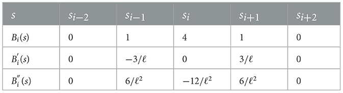
Table 1. Coefficients of third-degree B-splines and their derivatives at knots.

From Equation (10) and Table 1, we have

$\begin{array}{ll}\{\begin{array}{l}{(S)}_i^j={\alpha }_{i-1}^j+4{\alpha }_i^j+{\alpha }_{i+1}^j,\\ {(S_s)}_i^j=\frac{3}{\ell }\left({\alpha }_{i+1}^j-{\alpha }_{i-1}^j\right),\\ {(S_{ss})}_i^j=\frac{6}{{\ell }^2}\left({\alpha }_{i-1}^j-2{\alpha }_i^j+{\alpha }_{i+1}^j\right).\end{array}& (11)\end{array}$

At s = s_i undertaking the notation U(s_i, t_j+1) = Û(s_i) Equation (6) and introducing a fitting factor σ(s_i) in the resulting equation to handle the influence of perturbation parameter on solution profile, we have

$\begin{array}{ll}\{\begin{array}{l}{\mathcal{L}}_{\epsilon ,\gamma }^{N,M}Û(s_i)=\sigma (s_i)\epsilon {Û}_{ss}(s_i)+\gamma a(s){Û}_s(s_i)-p(s_i)Û(s_i)=g(s_i),\\ {Û}_0(s_i)={\theta }_0(s_i),0\le i\le N,\\ Û(0)=q^{j+1}(0),0\le j<M,\\ Û(1)=q^{j+1}(1),0\le j<M.\end{array}& (12)\end{array}$

In the corresponding time level, plugging Equation (11) at the knots into Equation (12) and simplifying, we obtain

$\begin{array}{r}{Y}_i^{-}{\alpha }_{i-1}^{j+1}+Y_i^c{\alpha }_i^{j+1}+Y_i^{+}{\alpha }_{i+1}^{j+1}=D_i^{-}{\alpha }_{i-1}^j+D_i^c{\alpha }_i\\ +D_i^{+}{\alpha }_{i+1}^j+{\ell }^2(f_i^j+f_i^{j+1}),i=0,1,2,...,N,& (13)\end{array}$

where

$\begin{array}{l}\begin{array}{l}{Y}_i^{-}=6{\sigma }_i\epsilon -3\ell \gamma a_i-{\ell }^2{p}_i,\\ Y_i^c=-12{\sigma }_i\epsilon -4{\ell }^2{p}_i,\\ Y_i^{+}=6{\sigma }_i\epsilon +3\ell \gamma a_i-{\ell }^2{p}_i.\end{array}\end{array}$

$\begin{array}{l}\begin{array}{l}{D}_i^{-}=-6{\sigma }_i\epsilon +3\ell \gamma a_i+{\ell }^2{p}_i,\\ D_i^c=12{\sigma }_i\epsilon +4{\ell }^2{p}_i,\\ D_i^{+}=-6{\sigma }_i\epsilon -3\ell \gamma a_i+{\ell }^2{p}_i.\end{array}\end{array}$

The fitting factor σ_i is given as [15, 16]

$\begin{array}{ll}{\sigma }_i=\frac{\gamma a_i\rho }{2}coth\left(\frac{\gamma a_i\rho }{2}\right),& (14)\end{array}$

where ρ = ℓ/ε.

At each (j + 1)th time level, this gives (N + 1) equations with (N + 3) unknowns $\left[{\alpha }_{-1}^{j+1},{\alpha }_0^{j+1},{\alpha }_1^{j+1},\cdots ,{\alpha }_{N+1}^{j+1}\right]$. Using boundary conditions in Equation (11) and the first and last equation, of Equation (13), we get

$\begin{array}{ll}Y{\alpha }_i^{j+1}=D{\alpha }_i^j+H,& (15)\end{array}$

where

$\begin{array}{l}Y=\left(\begin{array}{rr}\hfill (Y_0^c-4Y_0^{-})& (Y_0^{+}-Y_0^{-})\\ \hfill Y_1^{-}& Y_1^c& Y_1^{+}\\ \hfill & \hfill & \cdots & \cdots & \cdots \\ \hfill & \hfill & \hfill & \cdots & \cdots & \cdots \\ \hfill & \hfill & \hfill & \hfill & Y_{N-1}^{-}& Y_{N-1}^c& Y_{N-1}^{+}\\ \hfill & \hfill & \hfill & \hfill & \hfill & (Y_N^{-}-Y_N^{+})& (Y_N^c-4Y_N^{+})\end{array}\right),\end{array}$

$\begin{array}{l}D=\left(\begin{array}{rr}(D_0^c-4D{0}^{-})& (D_0^{+}-D_0^{-})\\ D_1^{-}& D_1^c& D_1^{+}\\ \hfill & \hfill & \cdots & \cdots & \cdots \\ \hfill & \hfill & \hfill & \cdots & \cdots & \cdots \\ \hfill & \hfill & \hfill & \hfill & D_{N-1}^{-}& D_{N-1}^c& D_{N-1}^{+}\\ \hfill & \hfill & \hfill & \hfill & \hfill & (D_N^{-}-D_N^{+})& (D_N^c-4D_N^{+})\end{array}\right),\end{array}$

$\begin{array}{c}H=\left(\begin{array}{c}{\ell }^2(f_0^j+f_0^{f+1})-Y_0^{-}{q}_0(t_{j+1})+D_0^{-}{q}_0(t_j)\\ {\ell }^2(f_1^j+f_1^{f+1})\\ ⋮\\ {\ell }^2(f_{N-1}^j+f_{N-1}^{f+1})\\ {\ell }^2(f_N^j+f_N^{f+1})-Y_N^{+}{q}_1(t_{j+1})+D_N^{+}{q}_1(t_j)\end{array}\right),\end{array}$

$\begin{array}{r}{\alpha }_i^{j+1}={\left({\alpha }_0^{j+1},{\alpha }_i^{j+1},{\alpha }_1^{j+1},\cdots ,{\alpha }_N^{j+1}\right)}^t,\text{and}\\ {\alpha }_i^j={\left({\alpha }_0^j,{\alpha }_i^j,{\alpha }_1^j,\cdots ,{\alpha }_N^j\right)}^t,\end{array}$

which is a diagonally dominant and non-singular matrix. Consequently, we get a exclusively solvable system of equations. So, we can solve the system in the study mentioned in the reference [15] for α′s, substituting these values into Equation (10), and we obtain the required approximate solution.

3 Convergence analysis

Lemma 5. [15] The B-Splines B₋₁, B₀, B₁, ..., B_N+1, satisfy the inequality

$\begin{array}{l}{\displaystyle \sum _{i=-1}^{N+1}}\left|B_i(s)\right|\le 10,s\in {\Omega }_s.\end{array}$

Proof. See [15]

Lemma 6. Let S(s) be the collocation approximation from the space of third-degree splines ${\xi }_3({\overline{\Omega }}_s)$ to the solution Û(s) of Equation (15) at the (j + 1)th time step. If g ∈ C²[0, 1], the parameter uniform error estimate is given by:

$\begin{array}{l}{\displaystyle \underset{0<\epsilon \le 1}{sup}}{\displaystyle \underset{0\le i\le N}{max}}|Û(s_i)-S(s_i)|\le C{\ell }^2,\end{array}$

where C is a positive constant independent of ε, μ, and N.

Proof. Let R(s) be the unique spline interpolate from ${\xi }_3({\overline{\Omega }}_N)$ to the solution Û(s_i) of the Equation (12) given by

$\begin{array}{ll}R(s)={\displaystyle \sum _{i=-1}^{N+1}}{\widehat{\alpha }}_i{B}_i(s).& (16)\end{array}$

If $g(s)\in C^2({\widehat{\Omega }}_s)$, $Û(s_i)\in C^4({\overline{\Omega }}_s)$, and adopting the Hall error estimates [17] for this case, we get

$\begin{array}{l}\Vert (Û(s)-R(s)){\Vert }_{\infty }\le c_0\Vert {Û}^{(4)}{\Vert }_{\infty }{\ell }^4,\\ \Vert ({Û}^{\prime }(s)-R^{\prime }(s)){\Vert }_{\infty }\le c_1\Vert {Û}^{(4)}{\Vert }_{\infty }{\ell }^3,\\ \Vert ({Û}^{″}(s)-R^{″}(s)){\Vert }_{\infty }\le c_2\Vert {Û}^{(4)}{\Vert }_{\infty }{\ell }^2,\end{array}$

where the c₀, c₁, and c₂ are the constants independent of ℓ and N. Therefore, from the estimates of the above equations and the collocating conditions ${\mathcal{L}}_{\epsilon ,\gamma }^{N,M}S(s_i)={\mathcal{L}}_{\epsilon ,\gamma }^MÛ(s_i)=g(s_i)$, it follows

$\begin{array}{r}\left|{ℒ}_{\epsilon ,\gamma }^{N,M}S(s_i)-{ℒ}_{\epsilon ,\gamma }^{N,M}R(s_i)\right|=\left|{ℒ}_{\epsilon ,\gamma }^M\widehat{U}(s_i)-{ℒ}_{\epsilon ,\gamma }^{N,M}R(s_i)\right|\\ \begin{array}{c}=\left|\epsilon \left({Û}^{″}(s_i)-\sigma (s_i)R^{″}(s_i)\right)+\gamma a(s_i)\left({Û}^{\prime }(s_i)-R^{\prime }(s_i)\right)\right|\end{array}\\ \begin{array}{c}\begin{array}{l}+\left|-p(s_i)\left(Û(s_i)-R(s_i)\right)\right|,\\ \begin{array}{c}=\left|\epsilon \left({Û}^{″}(s_i)-\sigma (s_i)R^{″}(s_i)\right)+\epsilon \sigma (s_i){Û}^{″}(s_i)-\epsilon \sigma (s_i){Û}^{″}(s_i)\right|\end{array}\end{array}\end{array}\\ +\left|\gamma a(s_i)\left({Û}^{\prime }(s_i)-R^{\prime }(s_i)\right)\right|+\left|p(s_i)\left(Û(s_i)-R(s_i)\right)\right|,\\ =\left|\epsilon \left(\sigma (s_i)-1\right){Û}^{″}(s_i)+\epsilon \sigma (s_i)\left({Û}^{″}(s_i)-R^{″}(s_i)\right)\right|\\ +\left|\gamma a(s_i)\left({Û}^{\prime }(s_i)-R^{\prime }(s_i)\right)\right|+\left|p(s_i)\left(Û(s_i)-R(s_i)\right)\right|,\\ \le \left|\epsilon \right||\sigma -1|{\Vert {Û}^{″}(s)\Vert }_{\infty }+\left|\epsilon \right|\left|\sigma \right|{\Vert {Û}^{″}(s)-R^{″}(s)\Vert }_{\infty }\\ +{\Vert \gamma a(s)\Vert }_{\infty }{\Vert {Û}^{\prime }(s)-R^{\prime }(s)\Vert }_{\infty }+{\Vert p(s)\Vert }_{\infty }{\Vert Û(s)-R(s)\Vert }_{\infty },\\ \le \left|\epsilon \right||\sigma -1|{\Vert {Û}^{(2)}(s)\Vert }_{\infty }+(\left|\epsilon \right|\left|\sigma \right|c_2{\ell }^2+{\Vert \mu a(s)\Vert }_{\infty }{c}_1{\ell }^3\\ +{\Vert p(s)\Vert }_{\infty }{c}_0{\ell }^4)\Vert {}_{\infty }{Û}^{(4)}\Vert .\end{array}$

Since ε ≪ 1 and as ℓ → 0, we obtain the following estimate

$\begin{array}{ll}|{\mathcal{L}}_{\epsilon ,\gamma }^{N,M}S(s_i)-{\mathcal{L}}_{\epsilon ,\gamma }^{N,M}R(s_i)|\le |\epsilon \Vert \sigma -1\Vert |{Û}^{(2)}{\Vert }_{\infty }.& (17)\end{array}$

From the power series expansion of hyperbolic cotangent function, we have $scoths\approx 1+\frac{s^2}{3}-\frac{s^4}{45}$ and then |scoths − 1| ≤ Cs². This and Equation (14) indicate

$\begin{array}{ll}|\sigma -1|\le C{\ell }^2.& (18)\end{array}$

Substituting Equation (19) in Equation (18), we get

$\begin{array}{ll}\Vert {\mathcal{L}}_{\epsilon ,\gamma }^{N,M}S(s)-{\mathcal{L}}_{\epsilon ,\gamma }^{N,M}R(s)\Vert \le C{\ell }^2.& (19)\end{array}$

Using relationship in Equation (15), ${\mathcal{L}}_{\epsilon ,\gamma }^{N,M}(Û(s_i)-R(s_i))$ yields,

$\begin{array}{ll}Y(\alpha -\widehat{\alpha })=(F-\widehat{F}),& (20)\end{array}$

where $\alpha ={\alpha }_i^{j+1},\overline{\alpha }={\overline{\alpha }}_i^{j+1}$,

$\begin{array}{l}\alpha -\widehat{\alpha }=({\alpha }_0-{\widehat{\alpha }}_0,{\alpha }_1-{\widehat{\alpha }}_1,\cdots ,{\alpha }_N-{\widehat{\alpha }}_N){,}^t\end{array}$

$\begin{array}{l}F=D{\alpha }_i^j+H,\end{array}$

$\begin{array}{l}F-\widehat{F}={({\ell }^2(g(s_0)-ĝ(s_0)),{\ell }^2(g(s_1)-ĝ(s_1)),\cdots ,{\ell }^2(g(s_N)-ĝ(s_N)))}^t.\end{array}$

Using Equation (20), we get

$\begin{array}{ll}\Vert F-\widehat{F}{\Vert }_{\infty }\le C{\ell }^4.& (21)\end{array}$

It is observed that the coefficient matrix A is diagonally dominant as they gratify the subsequent relations::

$\begin{array}{l}\left|y_{i,i}\right|-\left(\left|y_{i,i-1}\right|+\left|y_{i,i+1}\right|\right)=2p_i{\ell }^2\ge 2(\nu ){\ell }^2>0,asy(s)\ge \nu >0.\end{array}$

In addition, from the first and last rows of Y, we have

$\begin{array}{l}\begin{array}{ll}\left|y_{0,0}\right|-\left|y_{0,1}\right|=36{\sigma }_0+6p_0\ell ,& \left|y_{N,N}\right|-\left|y_{N,N-1}\right|=36{\sigma }_N-6p_N\ell .\end{array}\end{array}$

The above diagonal dominant property for smaller values of ℓ [18] gives

$\begin{array}{ll}\Vert Y^{-1}{\Vert }_{\infty }\le \frac{C}{{\ell }^2}.& (22)\end{array}$

From (20)-(22), we get

$\begin{array}{l}|{\alpha }_i-{\widehat{\alpha }}_i|\le C{\ell }^2,0\le i\le N.\end{array}$

Now to estimate $|{\alpha }_{-1}-{\widehat{\alpha }}_{-1}|$ and $|{\alpha }_{N+1}-{\widehat{\alpha }}_{N+1}|$, using the boundary conditions, we get

$\begin{array}{l}|{\alpha }_{-1}-{\widehat{\alpha }}_{-1}|\le C{\ell }^2.\end{array}$

$\begin{array}{l}|{\alpha }_{N+1}-{\widehat{\alpha }}_{N+1}|\le C{\ell }^2.\end{array}$

Therefore

$\begin{array}{ll}{\displaystyle \underset{-1\le i\le N+1}{max}}|{\alpha }_i-{\widehat{\alpha }}_i|\le C{\ell }^2.& (23)\end{array}$

The above inequality allows us to estimate: ‖S(s)−R(s)‖_∞, so ‖Û(s)−S(s)‖_∞. In specific,

$\begin{array}{ll}S(s)-R(s)={\displaystyle \sum _{i=-1}^{N+1}}({\alpha }_i-{\widehat{\alpha }}_i)B_i(s).& (24)\end{array}$

Thus, substituting Equation (24) and Lemma 5 in (25), we get

$\begin{array}{l}|S(s)-R(s)|\le {\displaystyle \underset{-1\le i\le N+1}{max}}|{\alpha }_i-{\widehat{\alpha }}_i|{\displaystyle \sum _{i=-1}^{N+1}}\left|B_i(s)\right|\le C{\ell }^2.\end{array}$

This gives

$\begin{array}{ll}\Vert S(s)-R(s){\Vert }_{\infty }\le C{\ell }^2.& (25)\end{array}$

Using the triangle inequality rule, we obtain

$\begin{array}{ll}\Vert Û(s)-S(s){\Vert }_{\infty }\le \Vert Û(s)-R(s){\Vert }_{\infty }+\Vert R(s)-S(s){\Vert }_{\infty }.& (26)\end{array}$

Using first term of Equation (17) and Equation (26) into Equation (27), we have

$\begin{array}{l}{\displaystyle \underset{0<\epsilon \le 1}{sup}}{\displaystyle \underset{0\le i\le N}{max}}|Û(s_i)-S(s_i)|\le C{\ell }^2.\end{array}$

Theorem 1. Let u(s_i, t_j) and S(s_i, t_j) be the solution of the problem (3) and the collocation approximation from the space ξ₃(Ω_s) to the solution u(s_i, t_j), respectively. If $g(s,t_j)\in C^2({\overline{\Omega }}_s)$,

$\begin{array}{l}\Vert u(s_i,t_j)-S(s_i,t_j)\Vert \le C({(\Delta t)}^2+{\ell }^2).\end{array}$

4 Test examples, numerical computations, and discussions

Some numerical experiments have been presented using the following examples.

Example 1. Consider the following problem of the form (1) [5, 6]

$\begin{array}{l}\{\begin{array}{l}\epsilon \frac{{\partial }^{2}u}{\partial s^2}+\gamma (1+s)\frac{\partial u}{\partial s}-u(s,t)-\frac{\partial u}{\partial t}=-u(s,t-1)\\ +16s^2(1-s^2),(s,t)\in {\Omega }_s\times (0,2],\\ u(s,t)=0,(s,t)\in {\Omega }_s\times (-1,0],\\ u(0,t)=0,u(1,t)=0,t\in (0,2].\end{array}\end{array}$

Example 2. Consider the following problem of the form (1) [5, 6]

$\begin{array}{l}\{\begin{array}{l}\epsilon \frac{{\partial }^{2}u}{\partial s^2}+\gamma (1+s(1-s)+t^2)\frac{\partial u}{\partial s}-(1+5st)u(s,t)-\frac{\partial u}{\partial t}\\ =-u(s,t-1)+s(1-s)(e^t-1),\\ (s,t)\in {\Omega }_s\times (0,2],\\ u(s,t)=0,(s,t)\in {\Omega }_s\times (-1,0],\\ u(0,t)=0,u(1,t)=0,t\in (0,2].\end{array}\end{array}$

Since the exact solution for Examples (1) and (2) is not exist, we use the double mesh principle to compute the maximum absolute errors, for each ε and μ, using the following formula [15, 19]:

$\begin{array}{ll}{E}_{\epsilon ,\gamma }^{N,M}={\displaystyle \underset{0\le i\le N;t\in \left[0,T\right]}{max}}|U^{N,M}(s_i,t_j)-U^{2N,2M}(s_i,t_j)|,& (27)\end{array}$

where $U^{N,M}(s_i,t_j)$ is the numerical solution with (N, M) mesh points, and $U^{2N,2M}(s_i,t_j)$ is the numerical solution at the finer mesh with (2N, 2M) mesh points. The (ε, γ)-uniform absolute errors are calculated using the following formula:

$\begin{array}{ll}{E}^{N,M}={\displaystyle \underset{\epsilon ,\gamma }{max}}{E}_{\epsilon ,\gamma }^{N,M}.& (28)\end{array}$

The numerical rate of convergence and the (ε, γ)-uniform rate of convergence are computed by using the following formulas, respectively.

$\begin{array}{ll}{\rho }_{\epsilon ,\gamma }^{N,M}={log}_2(\frac{E_{\epsilon ,\gamma }^{N,M}}{E_{\epsilon ,\gamma }^{2N,2M}})\text{ and }{\rho }^{N,M}={\displaystyle \underset{\epsilon ,\gamma }{max}}{\rho }_{\epsilon ,\gamma }^{N,M}.& (29)\end{array}$

The computed results by the proposed scheme and comparison with previous schemes for the considered problems are presented in Tables 2–5. From these tables, we observed that the presented method provides more accurate results than results in the study mentioned in the references [5] and [6]. 3-D view numerical simulation for Examples (1) and (2) is presented in Figures 1, 2, respectively. These figures show that as (ε, γ) goes very small, twin boundary layers formed at s = 0 and s = 1. We have plotted a log-log plot of the $E_{\epsilon ,\gamma }^{N,M}$ verses N in Figures 3A, B for (1)-(2), respectively. This figure shows that the scheme is stable and (ε, γ)−uniformly convergent.

Table 2

Table 2. Comparison of $E_{\epsilon ,\gamma }^{N,M}$ and ${\rho }_{\epsilon ,\gamma }^{N,M}$ for fixed γ = 10⁻⁴ and varying ε for Example (1) with the study mentioned in the reference [6] using Shishkin (S-) mesh and Bakhvalov-Shishkin (BS-) mesh.

Table 3

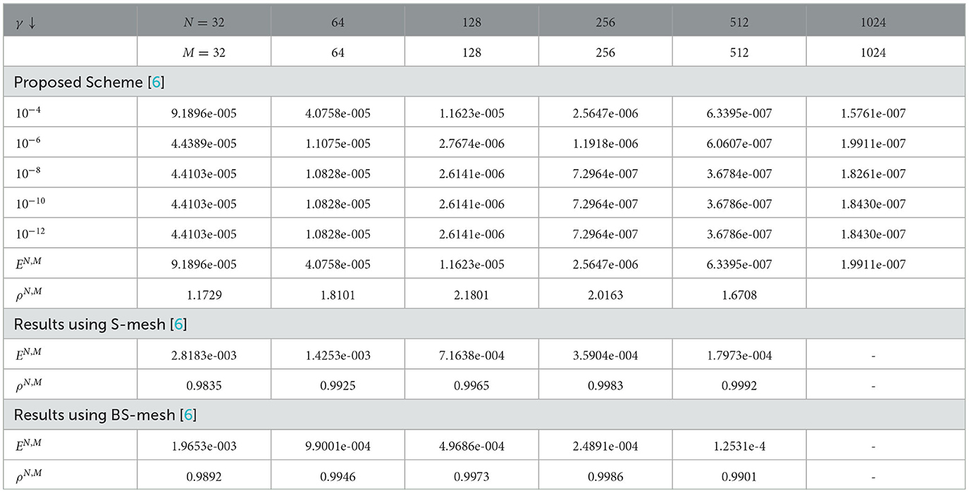
Table 3. Comparison of $E_{\epsilon ,\gamma }^{N,M}$, E^N,M, and ρ^N,M for ϵ = 10⁻⁴ and varying γ for Example (1) with the study mentioned in the reference [6] using S- mesh and BS- mesh.

Table 4

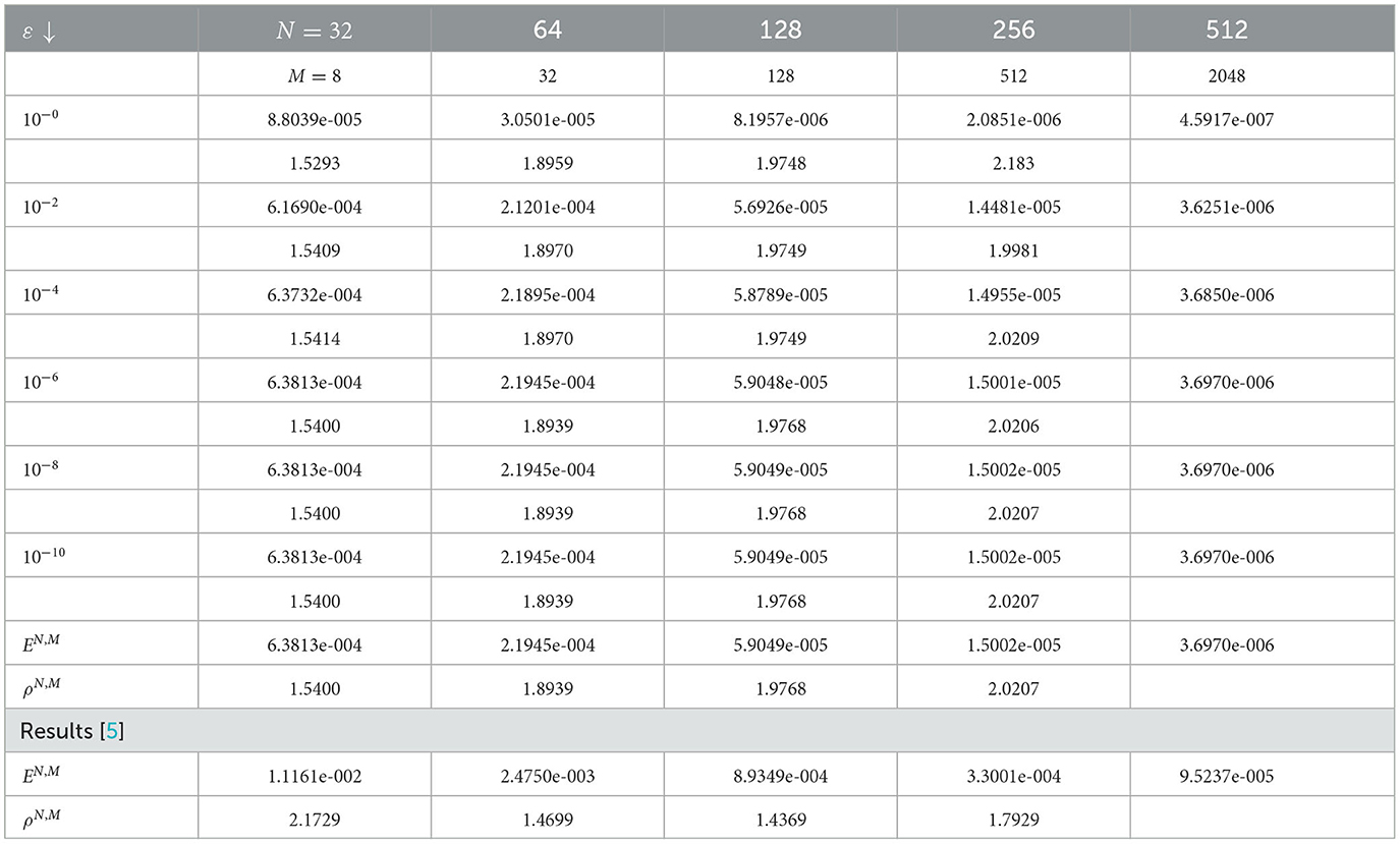
Table 4. Comparison of $E_{\epsilon ,\gamma }^{N,M}$ and ${\rho }_{\epsilon ,\gamma }^{N,M}$ for γ = 10⁻³ and varying ε for Example (2) with the results mentioned in the reference [5].

Table 5

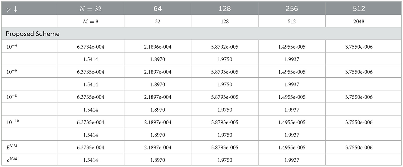
Table 5. Comparison of $E_{\epsilon ,\gamma }^{N,M}$, E^N,M, ${\rho }_{\epsilon ,\gamma }^{N,M}$, and ρ^N,M, for ϵ = 10⁻⁴ and varying γ for Example (2).

Figure 1

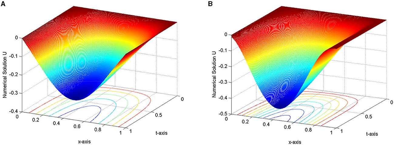
Figure 1. 3-D view numerical solution profile for Example 1 at N = 512 = M. (A) γ = 10⁻⁶, ε = 10⁻¹. (B) γ = 10⁻¹, ε = 10⁻⁶.

Figure 2

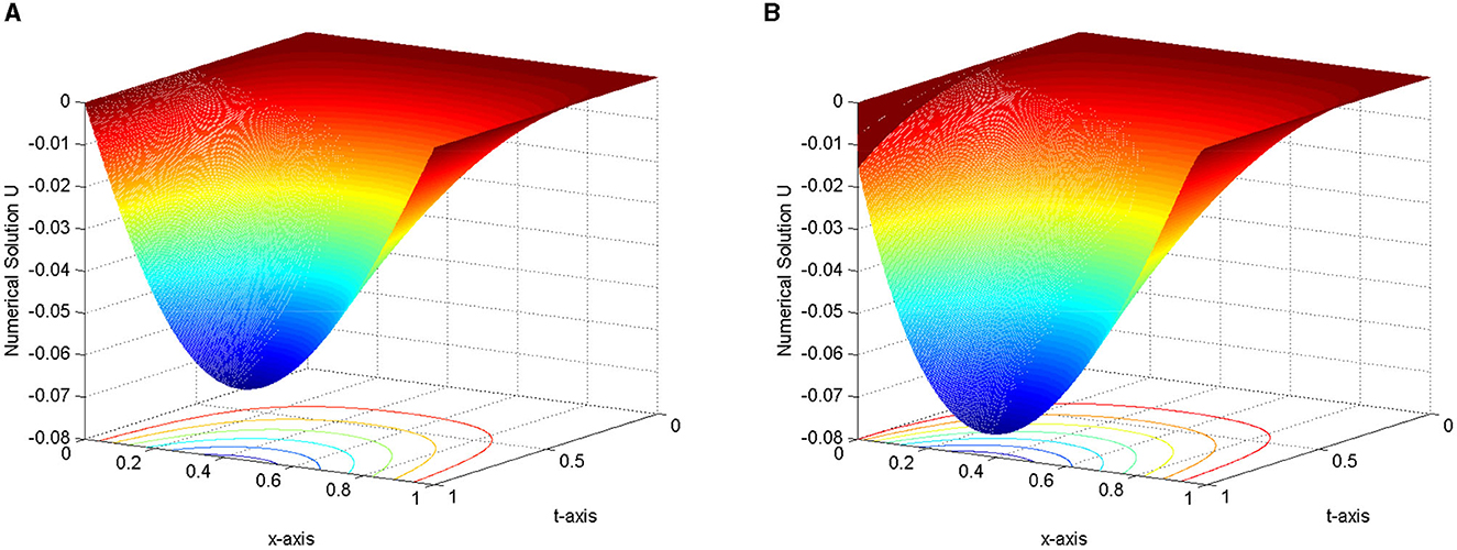
Figure 2. 3-D view numerical solution profile for Example 2 at N = 512 = M. (A) γ = 10⁻⁶, ε = 10⁻¹. (B) γ = 10⁻¹, ε = 10⁻⁶.

Figure 3

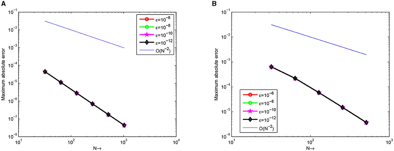
Figure 3. Loglog plot of the maximum point-wise errors for Examples 1 and 2 at different values of ε. (A) Example 1 with γ = 10⁻⁴. (B) Example 2 with γ = 10⁻³.

5 Conclusion

In this study, second order numerical method for the two-parametric singularly perturbed time delay parabolic problem on a uniform mesh is presented. The problem is discretized by the Crank-Nicolson method in time and the third-degree B-spline method in space variable. The presented scheme is proven to be an (ε, γ)−uniformly convergent accuracy of order O((Δt)² + ℓ²). To validate the theoretical findings, some test examples are considered. The computed results are in agreement with the theoretical investigations. Furthermore, the numerical results show that the presented scheme gives better results than available schemes in the literature.

Data availability statement

The raw data supporting the conclusions of this article will be made available by the authors, without undue reservation.

Author contributions

ITD: Conceptualization, Data curation, Formal analysis, Investigation, Methodology, Project administration, Resources, Software, Supervision, Validation, Visualization, Writing - original draft, Writing - review and editing. WGM: Conceptualization, Investigation, Methodology, Validation, Writing - review and editing. GDK: Investigation, Methodology, Validation, Writing - review and editing.

Funding

The author(s) declare that no financial support was received for the research, authorship, and/or publication of this article.

Acknowledgments

The authors would like to thank the editor and referees for careful reading and giving prolific comments.

Conflict of interest

The authors declare that the research was conducted in the absence of any commercial or financial relationships that could be construed as a potential conflict of interest.

Publisher's note

All claims expressed in this article are solely those of the authors and do not necessarily represent those of their affiliated organizations, or those of the publisher, the editors and the reviewers. Any product that may be evaluated in this article, or claim that may be made by its manufacturer, is not guaranteed or endorsed by the publisher.

References

1. Chen J, O'Malley RE Jr. On the asymptotic solution of a two-parameter boundary value problem of chemical reactor theory. SIAM J Appl Math. (1974) 26:717–29. doi: 10.1137/0126064

Crossref Full Text | Google Scholar

2. DiPrima RC. Asymptotic methods for an infinitely long slider squeeze-film bearing. J Lubricat Technol. (1968) 90:173–83. doi: 10.1115/1.3601534

Crossref Full Text | Google Scholar

3. Vasil'eva AB. Asymptotic methods in the theory of ordinary differential equations containing small parameters in front of the highest derivatives. USSR Comput Math Phys. (1963) 3:823–63. doi: 10.1016/0041-5553(63)90381-1

Crossref Full Text | Google Scholar

4. Bhathawala PH, Verma AP. A two-parameter singular perturbation solution of one dimension flow through unsaturated porous media. Proc Indian Natl Sci Acad. (1975) 43:380–4.

Google Scholar

5. Saini S, Kumar S, Kuldeep K, Kumar M. A robust numerical method for a two-parameter singularly perturbed time delay parabolic problem. Comput Appl Math. (2020) 39. doi: 10.1007/s40314-020-01236-1

Crossref Full Text | Google Scholar

6. Govindarao L, Sahu SR, Mohapatra J. Uniformly convergent numerical method for singularly perturbed time delay parabolic problem with two small parameters. Iran J Sci Technol Trans A Sci. (2019) 43:2373–83. doi: 10.1007/s40995-019-00697-2

Crossref Full Text | Google Scholar

7. Negero NT. A uniformly convergent numerical scheme for two parameters singularly perturbed parabolic convection-diffusion problems with a large temporal lag. Results Appl Math. (2022) 16:100338. doi: 10.1016/j.rinam.2022.100338

Crossref Full Text | Google Scholar

8. Negero NT. A parameter-uniform efficient numerical scheme for singularly perturbed time-delay parabolic problems with two small parameters. Partial Diff Equat Appl Math. (2023) 7:100518. doi: 10.1016/j.padiff.2023.100518

Crossref Full Text | Google Scholar

9. Vigo-Aguiara J, Natesan S. An efficient numerical method for singular perturbation problems. J Comput Appl Math. (2006) 192:132–41. doi: 10.1016/j.cam.2005.04.042

Crossref Full Text | Google Scholar

10. Natesan S, Vico-Acuiar J, Ramanujam N. A numerical algorithm for singular perturbation problems exhibiting weak boundary layers. Comput Math Appl. (2003) 45:469–79. doi: 10.1016/S0898-1221(03)80031-7

Crossref Full Text | Google Scholar

11. Vico-Acuiar J, Natesan S. A parallel boundary value technique for singularly perturbed two-point boundary value problems. J Supercomput. (2004) 27:195–206. doi: 10.1023/B:SUPE.0000009322.23950.53

Crossref Full Text | Google Scholar

12. Tian H. The exponential asymptotic stability of singularly perturbed delay differential equations with a bounded lag. J Math Anal Appl. (2002) 270:143–9. doi: 10.1016/S0022-247X(02)00056-2

Crossref Full Text | Google Scholar

13. Prenter P. Spline and Variational Methods. New York, NY: Wiley (1975).

Google Scholar

14. Schoenberg I. On spline functions. J Appl Comput Mech. (1966).

Google Scholar

15. Daba IT, Duressa GF. Collocation method using artificial viscosity for time dependent singularly perturbed differential–difference equations. Math Comput Simulat. (2022) 192:201–20. doi: 10.1016/j.matcom.2021.09.005

Crossref Full Text | Google Scholar

16. O'Malley RE. Singular Perturbation Methods for Ordinary Differential Equations. Berlin: Springer (1991). doi: 10.1007/978-1-4612-0977-5

Crossref Full Text | Google Scholar

17. Hall C. On error bounds for spline interpolation. J Approx Theory. (1968) 1:209–18. doi: 10.1016/0021-9045(68)90025-7

Crossref Full Text | Google Scholar

18. Varah JM. A lower bound for the smallest singular value of a matrix. Linear Algebra Appl. (1975) 11:3–5. doi: 10.1016/0024-3795(75)90112-3

Crossref Full Text | Google Scholar

19. Kadalbajoo MK, Yadaw AS. Parameter-uniform finite element method for two-parameter singularly perturbed parabolic reaction-diffusion problems. Int J Comput Methods. (2012) 9:1250047. doi: 10.1142/S0219876212500478

Crossref Full Text | Google Scholar