Persistence-based clustering with outlier-removing filtration

1 Introduction

Agglomerative hierarchical clustering is one of the main classes of clustering algorithms [1, 2]. It considers each data point as its own cluster and iteratively merges clusters. All state-of-the-art clustering algorithms require to choose parameters such as the number of clusters (K-means, spectral clustering, etc.), some thresholds (hierarchical clustering), or a density parameter for density-based clustering [DBSCAN [3, 4] and ToMATo [5]]. The choice of parameters can be problematic in some cases, especially when clustering is only one step in a larger algorithm.

Topological data analysis (TDA), and more specifically persistent homology [6, 7], has been a popular research subject over the last decades, with many applications [8]. The idea is to construct a sequence of simplicial complexes (a filtration) from given data and to study how its structure evolves when going through the filtration, using a tool called persistence diagram. The success of TDA is partly due to stability theorems, which state that close datasets will have close persistence diagrams, according to some distance between datasets/diagrams, ensuring in particular that TDA results are robust to noise. One of the most used filtrations is the Vietoris–Rips filtration, for which a stability theorem has been proved in [9].

Concretely, 0-dimensional persistent homology links data points until only one connected component is left. It thus naturally induces a hierarchical clustering algorithm as the one described in [10–12], that use the Vietoris–Rips filtration to study brain networks or co-occurrence networks, or the ToMATo algorithm [5], which combines TDA with a density-based approach. Persistent homology highlights important components of the data and is thus a suitable tool for threshold choice in hierarchical clustering. In this study, we introduce a new filtration for metric spaces¹ that adds information about the points' nearest neighbor to the persistence diagram which makes it easier to identify clusters on the diagram and to remove outliers. We prove its stability and use it to define a non-parametric algorithm to perform clustering with outlier removal.²

Section 2 is an introduction to TDA. In Section 3, we introduce our filtration and proved its stability. In Section 4, we present the algorithm and some experiments on point cloud and graph datasets.

2 Topological data analysis background

In this section, we introduce some notions of topological data analysis.

2.1 Simplicial complexes and filtrations

Definition 1. A k-simplex on a set X is an unordered tuple σ = [x₀, ..., x_k] of k+1 distinct elements of X. The elements x₀, ..., x_k are called the vertices of σ. If each vertex of a simplex τ is also a node of σ, then τ is called a face of σ. A simplicial complex K is a set of simplices such that any face of a simplex of K is a simplex of K. We call $S(X)$ the set of all simplices on X.

Definition 2. An increasing filtration³ of a simplicial complex K is a family of simplicial complexes (K_α)_α≥0 such that K₀ = ∅, $\alpha <{\alpha }^{\prime }\Rightarrow K_{\alpha }\subset K_{{\alpha }^{\prime }}$ and ⋃_α≥0K_α = K.

This definition is useful for theory, but in practice, the number of simplices is finite, in which case, we will only use a finite set of indices α_i such that $\varnothing =K^{{\alpha }_0}\subset K^{{\alpha }_1}\subset \cdots \subset K^{{\alpha }_m}=K$ and α_i ≤ α < α_i+1⇒K_αi = K_α. Without loss of generality, we can also assume that for all i, there exists a simplex σ_i+1∈K such that $K^{{\alpha }_{i+1}}=K^{{\alpha }_i}\cup \left\{{\sigma }_{i+1}\right\}$. See Figure 1 and [6, 7, 13] for examples of filtrations.

Figure 1

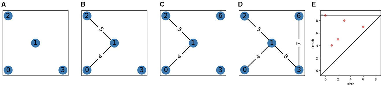
Figure 1. A filtration and its persistence diagram. (A) Steps 0 to 3 (add vertices 0, 1, 2, and 3). (B) Steps 4 and 5 (add edges 4 and 5). (C) Step 6 (add vertex 6). (D) Steps 7 and 8 (add edges 7 and 8). (E) 0-dimensional persistence diagram.

In clustering applications, data are a (finite) metric space (X, d). A common and easily computable filtration on X is the Vietoris–Rips filtration VR(X) = (VR(X, α))_α≥0 defined for all simplices σ by:

$\begin{array}{l}\forall \sigma \in S(X),\sigma \in VR(X,\alpha )\iff \forall x,y\in \sigma ,d(x,y)\le \alpha \end{array}$

The main idea of TDA is to build a filtration on top of the data and study how the structure of the simplicial complexes evolves while increasing the filtration parameter using persistent homology. Our clustering algorithm only requires 0-dimensional persistent homology, which we will explain in terms of connected components. Persistent homology is defined for higher dimensions in Section 2.3 (we define it for the sake of completeness, as Theorem 10 is about all dimensions).

2.2 0-dimensional persistent homology

Let ${(K^{{\alpha }_i})}_{0\le i\le m}$ be a filtration. For each index i, we go from $K^{{\alpha }_i}$ to $K^{{\alpha }_{i+1}}$ by adding a simplex σ_i+1 to $K^{{\alpha }_i}$. If σ_i+1 is a vertex, then it creates a new connected component in $K^{{\alpha }_{i+1}}$, and we say that this component is born at α_i+1. If σ_i+1 is an edge, it links two vertices that where already in $K^{{\alpha }_i}$ (by definition of a simplicical complex). If those vertices belonged to different connected components in $K^{{\alpha }_i}$, they become one component in $K^{{\alpha }_{i+1}}$: we say that one of the two components (the one with the lowest birth date, by convention) absorbed the younger one, and that the younger one died at α_i+1. In all other cases, there is no change in connected components when adding σ_i+1 (changes are made in higher dimensional homology, see Section 2.3). At the end of the filtration, all remaining components die at α = ∞. The 0-dimensional persistence diagram of a filtration is defined as the multiset of all pairs (birthdateanddeathdate) obtained by the above construction, counted with multiplicity, along with all pairs (x, x) with infinite multiplicity.

See Figures 1A–E for an example of persistence diagram. If (b, d) is a point of a persistence diagram, we call d−b its persistence (or the persistence of the corresponding connected component).

A distance between persistence diagrams can be defined as follows:

Definition 3. The bottleneck distance between diagrams D and D′ is defined as:

$d_B(D,D^{\prime })={\displaystyle \underset{\gamma \in \Gamma (D,D^{\prime })}{inf}}{\displaystyle \underset{p\in D}{sup}}||p-\gamma (p){||}_{\infty }$

where Γ(D, D′) is the set of bijections from D to D′, where a point of multiplicity m is treated as m points, and where ||p−q||_∞ = |x_p−x_q| when p = (x_p, y_p), q = (x_q, y_q) and y_p = y_q = +∞.

Note that it is necessary to include the diagonal in persistence diagrams so there exists bijections between diagrams that do not have the same number of persistent pairs.

2.3 Persistent homology in any dimension

2.3.1 Simplicial homology

Let K be a simplicial complex with maximal simplex dimension d, 𝔽 be a field and 0 ≤ k ≤ d.

Definition 4. The space C_k(K) of k-chains is defined as the set of formal sums of k-simplices of K with coefficients in F, that is to say, if all the k-simplices of K are σ₁, …, σ_nk, all the elements of the form:

$c={\displaystyle \sum _{i=1}^{n_k}}{a}_i{\sigma }_i,a_i\in 𝔽.$

C_k(K) is a vector space whose addition and scalar multiplication are naturally defined as follows: if $c=\sum _{i=1}^{n_k}{a}_i{\sigma }_i$ and $c^{\prime }=\sum _{i=1}^{n_k}{a}_i^{\prime }{\sigma }_i$, then:

$c+c^{\prime }={\displaystyle \sum _{i=1}^{n_k}}(a_i+a_i^{\prime }){\sigma }_i.$

and for λ ∈ 𝔽,

$\lambda c={\displaystyle \sum _{i=1}^{n_k}}(\lambda a_i){\sigma }_i.$

Using a field F gives the more general definition, but from now on, we will only consider 𝔽 = ℤ/2ℤ, so the coefficients are modulo 2, which allows to avoid orientation considerations.

Definition 5. Let σ = [v₁, …, v_k] be a k-simplex with vertices v₁, …, v_k, and $\left[v_1,\dots ,\widehat{v_i},\dots ,v_k\right]$ be the (k−1)-simplex spanned by those points minus v_i. The boundary operator ∂ is defined as:

$\partial :\{\begin{array}{l}{C}_k(K)\to C_{k-1}(K)\\ \sigma \mapsto \partial \sigma ={\displaystyle {\sum }_{i=1}^k{\left(-1\right)}^i}[v_1,\dots ,\widehat{v_i},\dots ,v_k].\end{array}$

We have the following sequence of linear maps:

$\left\{0\right\}\to C_d(K)\stackrel{\partial }{\to }{C}_{d-1}(K)\stackrel{\partial }{\to }\dots \stackrel{\partial }{\to }{C}_1(K)\stackrel{\partial }{\to }{C}_0(K)\stackrel{\partial }{\to }\left\{0\right\}.$

They satisfy ∂°∂ = 0 : we call such a sequence of maps a chain complex. This constitutes the setup for homology. We can now define cycle and boundaries, homology groups, and Betti numbers.

Definition 6. We define the set Z_k(K) of k-cycles of K as :

$Z_k(K)=Ker(\partial :C_k(K)\to C_{k-1}(K))$

and the set B_k(K) of k-boundaries of K as :

$B_k(K)=Im(\partial :C_{k+1}(K)\to C_k(K)).$

We have B_k(K) ⊂ Z_k(K) ⊂ C_k(K), so we can define the k^th homology group as:

$H_k(K)=Z_k(K)/B_k(K)$

and the k^th Betti number:

${\beta }_k(K)=dim(H_k(K)).$

β_k represents the number of k-dimensional “holes”. For example, β₀ is the number of connected components of K, β₁ is the number of loops, and β₂ is the number of voids. Betti numbers of simplicial complexes are computable using a filtration, see [7] for the algorithm.

2.3.2 Persistent homology

Persistent homology considers studying the evolution of homology groups while increasing the filtration parameter.

Let ${(K^{{\alpha }_i})}_{0\le i\le m}$ be a filtration such that for each index i, we go from $K^{{\alpha }_i}$ to $K^{{\alpha }_{i+1}}$ by adding a simplex σ_i+1 to $K^{{\alpha }_i}$.

We call $C_k^i,Z_k^i,B_k^i,H_k^i,and{\beta }_k^i$ the respective spaces of k-chains, k-cycles, k-boundaries, k^th homology group and k^th Betti number of Kⁱ. The goal is to follow the evolution of $H_k^i$ as i increases. It can be shown [7] that when a k-simplex σ_i+1 (k>0) is added, it either creates a new homology class in $H_k^{i+1}$ (i.e., a new k-cycle that is independent of those of $H_k^i$) or it closes a k−1-dimensional hole of $H_{k-1}^{i-1}$, so $H_{k-1}^i$ has one less homology class than $H_{k-1}^{i-1}$, in that case, we say that σ_i+1 killed a homology class (by convention, we always consider that when two classes merge, the younger class gets killed). If k = 0, each new vertex creates a homology class in H₀.

The final result of persistent homology is the set of all so-called persistent pairs (σ_l(j), σ_j) such that for each j, σ_l(j) creates a component and σ_j kills it. We say that the persistence (or lifetime) of such a pair is j−l(j)−1. The algorithms to compute them are described in detail in [7]. The k-dimensional persistence diagram is the set of points of coordinates (α_l(j), α_j) such that σ_l(j) is a k-simplex (counted with multiplicity). The points of the diagonal y = x are added with infinite multiplicity (it is useful to define distances). The bottleneck distance between two k-dimensional persistence diagrams is defined exactly as in Definition 3.

3 Nearest Neighbor Vietoris-Rips filtration and stability

In this section, we introduce a new filtration: the Nearest Neighbor Vietoris-Rips (NNVR) filtration, and prove its stability.

Definition 7. Let (X, d) be a metric space. The Nearest Neighbor Vietoris-Rips filtration NNVR(X, α)_α≥0 is defined by:

$\begin{array}{l}\forall x\in X,x\in NNVR(X,\alpha )\iff \alpha \ge {\displaystyle \underset{y\in X,y\ne x}{inf}}d(x,y)\end{array}$

and for all k-simplices σ with k ≥ 1:

$\begin{array}{l}\sigma \in NNVR(X,\alpha )\iff \sigma \in VR(X,\alpha )\end{array}$

This means that the NNVR filtration is the same as the VR filtration except for 0-simplices, which all enter the VR filtration at α = 0, whereas they enter the NNVR filtration when α is equal to the distance to their nearest neighbor. It is easy to verify that NNVR is indeed a filtration. Figure 2 shows an example of NNVR filtration.

Figure 2

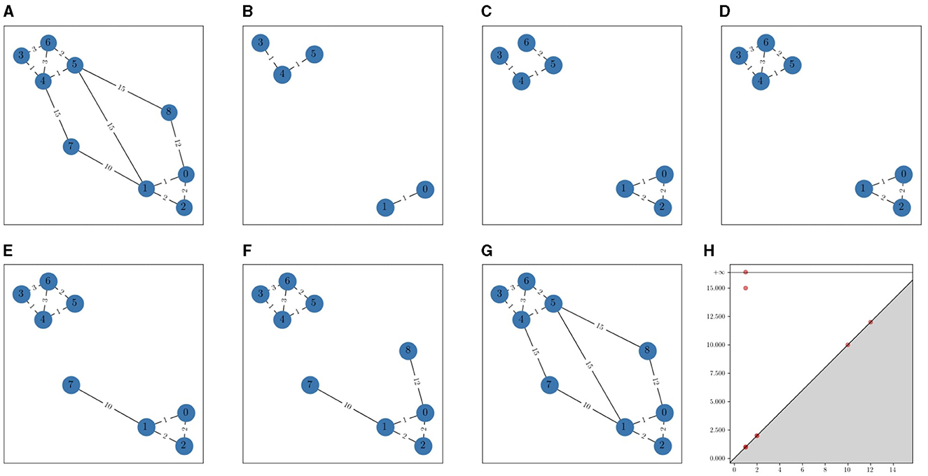
Figure 2. An example of NNVR filtration. The edge weights represent the distance between vertices. For each value of α, vertices and edges with filtration value equal to α are added. (A) Full graph. (B) α = 1. (C) α = 2. (D) α = 3. (E) α = 10. (F) α = 12. (G) α = 15. (H) α = Persistence diagram.

The stability theorem for the VR filtration is proved in [9], we use the same framework as they did to adapt the proof to the NNVR filtration. The theorem states that the NNVR filtration is stable with respect to the Gromov–Hausdorff distance [14], which we define below, along with the notions required to prove the theorem.

Definition 8. Let X, Y be two sets and C ⊂ X × Y. For any A ⊂ X and B ⊂ Y, we note C(A) = {y ∈ Y:∃x ∈ A, (x, y) ∈ C} and C^⊤(B) = {x ∈ X:∃y ∈ B, (x, y) ∈ C}. C is called a correspondence between X and Y if C(X) = Y and

C^⊤(Y) = X.

Definition 9. Let (X, d_X) and (Y, d_Y) be metric spaces and C be a correspondence between X and Y. The distortion of C is defined as

$\begin{array}{l}dis(C)=sup\left\{|d_X(x,x^{\prime })-d_Y(y,y^{\prime })|:(x,y),(x^{\prime },y^{\prime })\in C\right\}.\end{array}$

The Gromov–Hausdorff distance between X and Y is:

$\begin{array}{l}{d}_{GH}(X,Y)=\frac{1}{2}inf\\ \left\{dis(C):\text{C is a correspondence between X and Y}\right\}.\end{array}$

We now state the stability theorem.

Theorem 10. Let (X, d_X) and (Y, d_Y) be totally bounded metric spaces. Let D_X (resp. D_Y) be the persistence diagram of NNVR(X) (resp. NNVR(Y)). Then:

$\begin{array}{l}{d}_B(D_X,D_Y)\le 2d_{GH}(X,Y).\end{array}$

To prove this theorem, we introduce simplicial correspondences and use results from [9].

Definition 11. Let ${(K^X)}_{\alpha \ge 0}$ (resp. ${(K^Y)}_{\alpha \ge 0}$) be a filtration of a simplicial complex on a set X (resp. Y). A correspondence C is called ε-simplicial, if

• For any α ≥ 0 and simplex $\sigma \in K_{\alpha }^X$, any finite subset of C(σ) is a simplex of $K_{\alpha +\epsilon }^Y$.

• For any α ≥ 0 and simplex $\sigma \in K_{\alpha }^Y$, any finite subset of C^⊤(σ) is a simplex of $K_{\alpha +\epsilon }^X$.

Proposition 4.2 from [9] states that if there is an ε-simplicial correspondence between two filtered metric spaces X and Y, then there exists a so-called ε-interleaving between the persistent homology groups of X and Y which is a family of linear maps between homology groups $H_k(K_{\alpha }^X)\to H_k(K_{\alpha +\epsilon }^Y)$ and $H_k(K_{\alpha }^Y)\to H_k(K_{\alpha +\epsilon }^X)$ for all α, that commute with the persistence structure. Theorem 2.3 from [9] states that if there exists such an ε-interleaving then ε is an upper bound on the bottleneck distance.⁴ The following lemma synthesizes those results.

Lemma 12. Let ${(K^X)}_{\alpha \ge 0}$ (resp. ${(K^Y)}_{\alpha \ge 0}$) be a filtration of a finite simpicial complex on a totally bounded metric space X (resp. Y), with persistence diagrams D_X and D_Y. If there exists an ε-simplicial correspondence, then d_B(D_X, D_Y) ≤ ε.

Proof of Theorem 10: Let ε > 2d_GH(X, Y). There exists a correspondence C such that $dis$(C) ≤ ε. Let us show that C is ε-simplicial.

Let α ≥ 0, σ be a simplex of NNVR(X, α) and τ be a finite subset of C(σ).

Case 1: τ only has one element: τ = [y]. There exists x∈σ such that y∈C(x) and a sequence ${(x_n)}_{n\in \mathbb{N}}\in X^{\mathbb{N}}$ such that 0 < d_X(x,x_n) and (d_X(x,x_n))_n∈ℕ converges to a value lower than or equal to α. Moreover, there exists a sequence ${(y_n)}_{n\in \mathbb{N}}\in Y^{\mathbb{N}}$ such that for all n, y_n ∈ C(x_n). Then:

$\forall n\in \mathbb{N},{\displaystyle \underset{z\in Y,z\ne y}{inf}}{d}_Y(y,z)\le d_Y(y,y_n)\le d_X(x,x_n)+\epsilon$

So: $\underset{z\in Y,z\ne y}{inf}{d}_Y(y,z)\le \alpha +\epsilon$ and τ = [y] ∈ NNVR(Y, α + ε).

Case 2: τ = [y₀, ..., y_k], k≥1. For all i, j, there exists x_i, x_j ∈ σ such that y_i ∈ C(x_i) and y_j ∈ C(x_j). Then :

$d_Y(y_i,y_j)\le d_X(x_i,x_j)+\epsilon \le \alpha +\epsilon \text{and }\tau \in NNVR(Y,\alpha +\epsilon )$

where the last inequality holds because [x_i, x_j]∈NNVR(X, α).

The same proof shows that if σ is a simplex in NNVR(Y, α), then all finite subsets of C^⊤(σ) are simplices of NNVR(X, α+ε). So, C is ε-simplicial and Lemma 12 ends the proof.

4 Outlier-removing clustering

4.1 Algorithm

Our clustering algorithm relies on the 0-dimensional persistent homology construction described in Section 2.2. The idea is to construct the 0D persistence diagram of the NNVR filtration of the data, then use it to choose a birth threshold (which tells us which points are outliers) and a persistence threshold (which tells us what the clusters are). The thresholds can be chosen manually or automatically. If they are chosen using a non-parametric procedure, then the whole clustering algorithm is non-parametric (see next section for more details). The clustering algorithm works as follows:

• Input: a finite metric space (X, d).

• Compute the filtration NNVR(X) and its 0-dimensional persistence diagram.

• Choose a birth threshold and a persistence threshold.

• Mark all points whose birth dates are above the birth threshold as outliers. Let Y be the remaining points.

• Compute 0-dimensional persistent homology on NNVR(Y), but do not add edges that would merge components whose persistence is above the persistence threshold.

• Output: a simplicial complex, where each connected component is a cluster.

The benefit of using the NNVR filtration is that, compared to the VR filtration, it separates outliers from essential components on the persistence diagram. Components corresponding to outliers indeed have late death dates in both filtrations as they are far away from other points. Thus, they give very persistent points with the VR filtration (where every birth date is 0), which can be hard to distinguish from other persistent points (as illustrated below). The NNVR filtration moves them to the right of the persistence diagram. Note that, if there are no outliers, the same algorithm can be used with the VR filtration and no birth threshold.

Seeing (X, d) as a graph with n vertices and m edges, the filtration can be computed in O(m) (the filtration value of each vertex is the distance to its nearest neighbor, and the filtration value of each edge is its weight, so reading the m edge weights is enough to compute the filtration). Computing 0D persistent homology requires to compute a minimal spanning tree, which can be done in O(m$log(max$(m, n))) using Kruskall's algorithm. An algorithm to choose the thresholds (such as max-jump, described below) should work in O(n), as there are n points on the persistence diagram. So, the overall complexity of the method is O(m$log(max$(m, n))), so O(n²$log$(n)) in the worst case, as m ≤ n², with equality if the whole distance matrix is computed (in Euclidean spaces, for example).

4.2 Choice of thresholds

After computing the persistence diagram D, two thresholds are needed: a birth threshold, which is a threshold on the list of birth dates of points on the diagram, and a persistence threshold, which is a threshold on the list of persistence of points on the diagram. The choice of the birth threshold determines which points are considered as outliers: if a point on the persistence diagram has a birth date above the threshold, we exclude the corresponding point in X and detect it as an outlier. The choice of the persistence threshold determines which components are significant enough to be considered as clusters. The number of points whose persistence is above the threshold is the number of detected clusters.

A natural method to choose the birth and persistence thresholds is to apply the max-jump algorithm to the list of birth dates and to the list of persistence values (without the point of infinite persistence). The algorithm is defined in Algorithm 1.

Algorithm 1

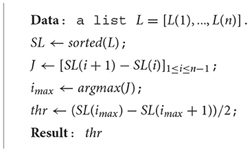
Algorithm 1. Max-jump algorithm.

The idea behind this algorithm is to separate significant values from non-significant ones by using the biggest variation. It is fully non-parametric, and will always output at least two clusters (one corresponding to the infinite persistence point, and at least one point above the persistence threshold). A drawback of this method is that it can output a persistence threshold that is too low if clusters are not at the same distance from one another (see point cloud 5 in section 4.3. for an example).

We propose two possible solutions to this problem, which introduce the choice of a parameter. The first one is to apply a sigmoid function $s_{\lambda }:x\mapsto \frac{1}{1+e^{-\lambda x}}$ to the normalized list $\frac{L}{max(L)}$ before using max-jump. The normalization makes the data vary from 0 to 1, which makes it easier to choose a unique parameter λ for a whole dataset, and the sigmoid function pushes significant values close to 1, which can lead to a lower threshold than the one obtained with max-jump. The second alternative we propose is using OTSU's method [15] for gray-level threshold selection. This requires to choose a number of bins for the histograms, which we set to 1,024 by default. As the persistence distribution is skewed, we apply the algorithm twice and remove values under the threshold after each iteration. The point cloud experiments on Section 4.3 illustrate how those alternatives can improve clustering. For every other dataset, we will always use max-jump by default. Other methods can be preferred depending on the application, to make use of prior knowledge on the data (for example, knowledge about the expected number of clusters or their size).

Figure 3 shows the thresholded persistence diagram (with max-jump) and the results of our algorithm on the graph from Figure 2.

Figure 3

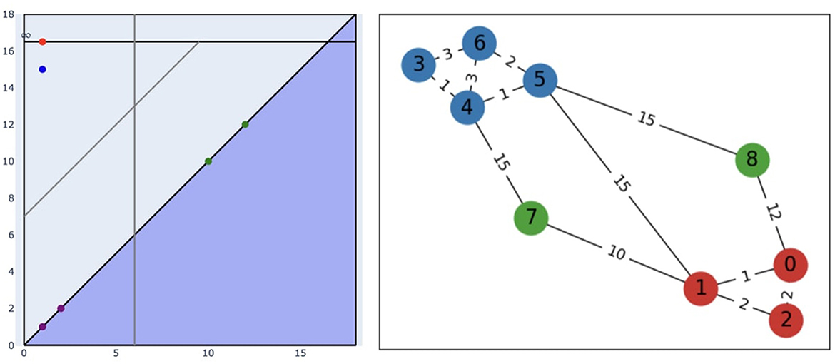
Figure 3. (Left) The persistence diagram from Figure 2 with both thresholds chosen with max-jump. The vertical gray line represents the birth threshold, the gray line parallel to the diagonal represents the persistence threshold (as the persistence of a point is proportional to its distance to the diagonal). (Right) Clusters (blue and red) and outliers (green) obtained with our algorithm. A point of a given color on the diagram represents the component that contains the nodes of this color on the graph.

4.3 Experiments

We applied our algorithm to the karate club graph, which is a classical example for community detection in networks [16], to point clouds from the scikit-learn documentation⁵ to which we added four outliers (one in each corner), and to synthetic graph datasets. Results were evaluated using the Rand index [17], which is the ratio of the number of correctly labeled points over the total number of points, ignoring label permutations (so perfect clustering gives a Rand index of 1 and the index is close to 0 for bad clustering).

4.3.1 Karate club graph

The karate club graph shows the interactions between the 34 members of a karate club (nodes 0–33). Each interaction is represented by an edge with a weight between 1 and 7 (a high weight means more interaction). After a conflict between the instructor (node 0) and administrator (node 33), the club split up into two groups: one with the instructor and one with the administrator. The goal is to predict those groups based on the interaction. We added 10 outliers (nodes 34–43, that could represent people outside the club), each one with two edges randomly linking it to other nodes with a random weight between 0.5 and 1. We inverted the weights of the edges to get a new weighted graph and used the shortest-path distance.

The results are shown in Figure 4 along with persistence diagrams for the NNVR and VR filtrations, and results obtained with the Louvain Community Detection Algorithm [18], which is a modularity optimization method [we used the NetworkX [19] implementation with default parameters]. The Rand indices are 0.95 for the NNVR method, 0.65 for the VR method, and 0.73 for the Louvain method. Note that points from both diagrams have the same death dates, so outliers have a higher persistence than relevant points on the VR diagram, which is not the case on the NNVR diagram. The algorithm exactly recovers the true clusters for all nodes, except nodes 5, 6, 16, and 10, that form a cluster. This can be explained by the fact that node 16 is not linked to node 0 and only has two links to 5 and 6, and the edges (5,6) and (5,10) are, respectively, heavier than (5,0) and (10,0). This point is more persistent than the blue one on Figure 4 because of the proximity between nodes 8 and 33.

Figure 4

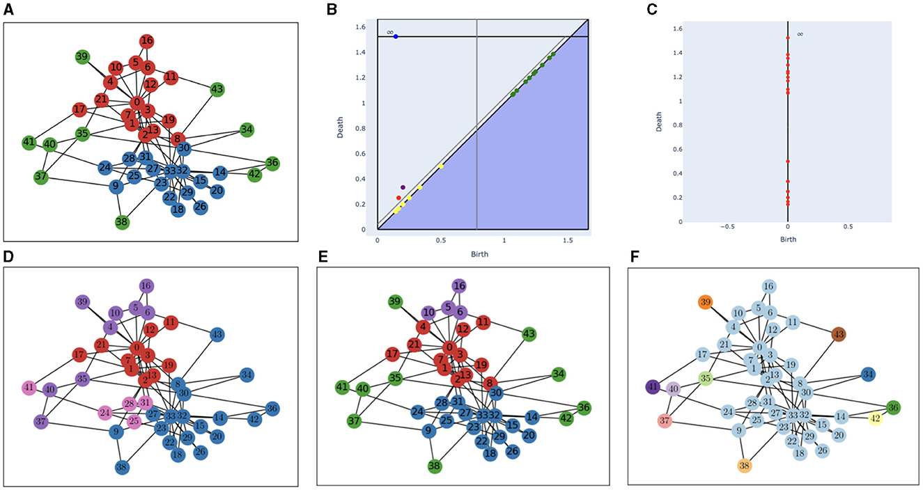
Figure 4. (A) Ground truth for the karate club graph with additional outliers, (B) persistence diagram of the NNVR filtration, (C) persistence diagram of the VR filtration, (D) clusters obtained with the Louvain Community Detection Algorithm, (E) clusters obtained with the NNVR algorithm, and (F) clusters obtained with the VR algorithm. On (B), the two gray lines represent the two thresholds, the blue (resp. red, purple) point corresponds to the blue (resp. red, purple) cluster on the graph, green points correspond to outliers, and yellow points are below the persistence threshold.

4.3.2 Point clouds

In the case of point clouds, the metric space is a set of points in 2D equipped with the Euclidean distance. Figures 5, 6 and Table 1 show the results of 10 clustering algorithms [3, 20–27], and three versions of our algorithm that all use max-jump to choose the birth threshold but different methods (described above) for the persistence threshold: one using max-jump, one using it after applying a sigmoid with parameter 4, and one using OTSU. We also test our algorithm with the VR filtration (and max-jump persistence threshold), on three point clouds. For all algorithms, we used the same parameters as the ones used in the scikit-learn documentation.

Figure 5

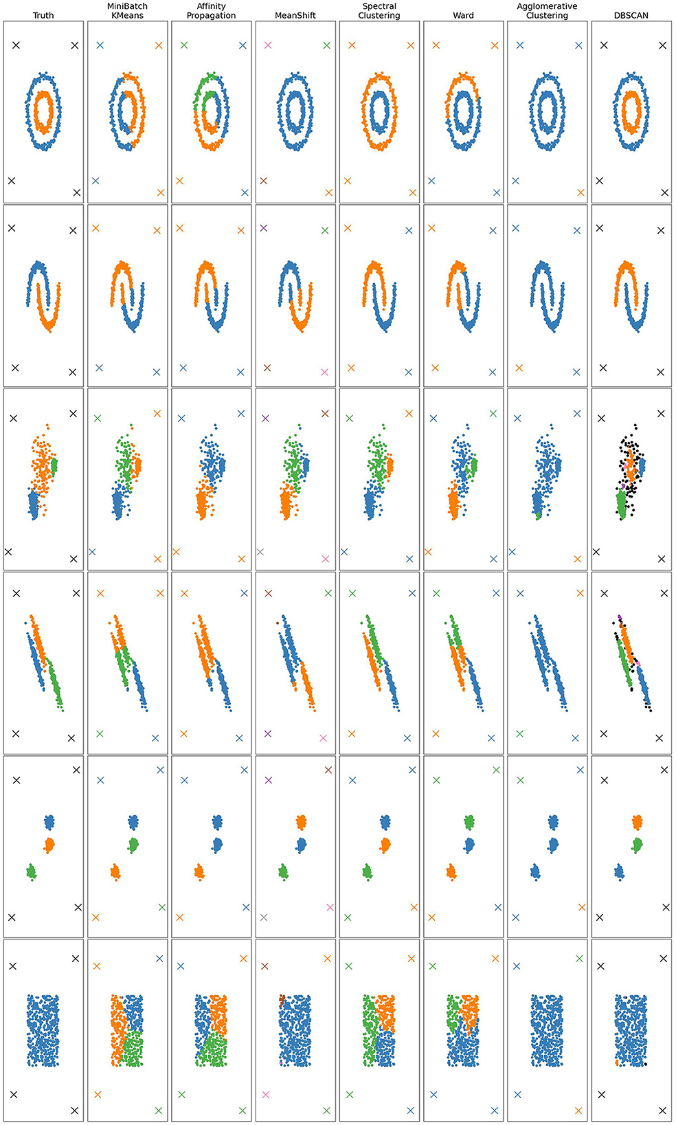
Figure 5. Clustering results for six point clouds obtained with several methods. Points marked with an X are outliers.

Figure 6

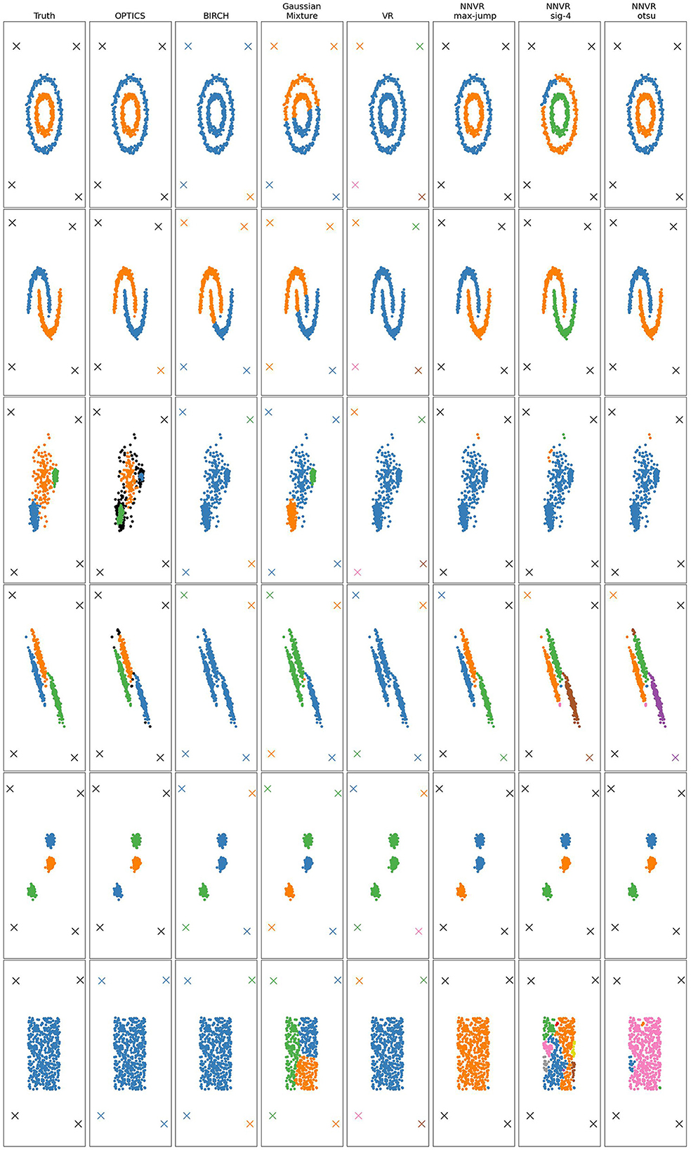
Figure 6. Clustering results for six point clouds obtained with several methods, including the NNVR filtration with max-jump, sigmoid of parameter 4 and OTSU, and VR filtration. Points marked with an X are outliers.

Table 1

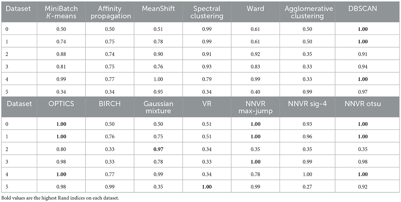
Table 1. Rand indices for the 14 clustering algorithms applied to the six datasets represented on Figures 5, 6.

The NNVR algorithm with max-jump performs almost perfectly on datasets 1, 2, 4, and 6. On dataset 5, the persistence threshold is too high so the algorithm detects two clusters instead of three, which is not the case for the sigmoid and OTSU methods, which work perfectly on this dataset. The drawback of the sigmoid and OTSU methods is that they tend to choose more clusters than max-jump and can thus choose too many such as for datasets 4 and 6 (and 1 and 2 for the sigmoid). Density-based methods outperform the others on dataset 3. Dataset 6 shows that our algorithm cannot output only one cluster. The only methods capable of detecting outliers are DBSCAN, OPTICS, and our NNVR method. Our method only fails to detect two of the four outliers on dataset 4. DBSCAN and OPTICS detect too many outliers on datasets 3 and 4.

4.3.3 Synthetic graphs

We used the NetworkX's [19] $random\_partition\_graph$ function to generate synthetic graph datasets with a number of clusters varying from 2 to 10 and containing outliers. This functions takes as input the size of each cluster, a probability p_in, and a probability p_out. It outputs a random graph where each edge has a probability p_in of existing between two nodes from the same cluster, and p_out if they are from different clusters. The data were generated as follows:

• Fix a number of iterations n and a number of clusters k, p_in = 0.3 and p_out = 0.01.

• Set the size of each cluster to 5 plus a random integer between −3 and 3.

• Add five clusters of size 1 (the outliers).

• Generate n graphs with the above procedure, and add their adjacency matrices together. The resulting matrix is the adjacency matrix of a weighted graph G_{n, k}.

See Figure 7 for examples. Table 2 shows the results obtained with our algorithm (using max-jump for both thresholds) and with the Louvain method [18], for n = 30, 40, 50 and k varying from 2 to 10. Our method performs better than Louvain's on 5 and 6 graphs out of 9 for n = 30 and 40, respectively, and for higher values of n, when clusters are denser, our method always detects the right clusters and outliers.

Figure 7

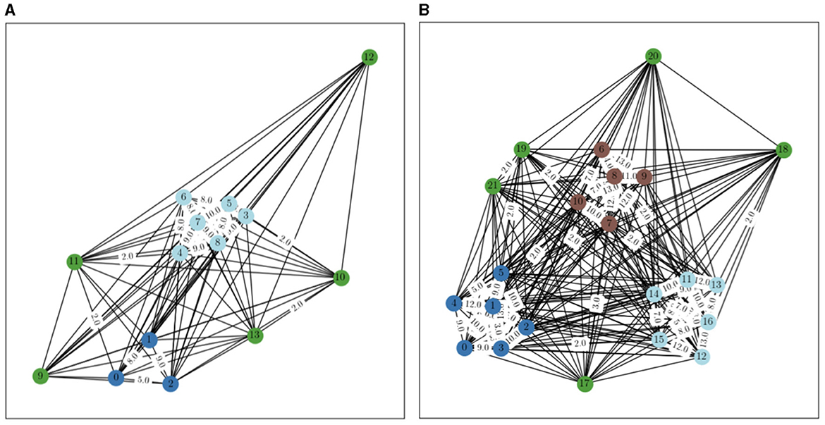
Figure 7. Generated graphs with n = 30, with 2 clusters on (A) and 3 on (B). Edges without a label have a weight of 1.

Table 2

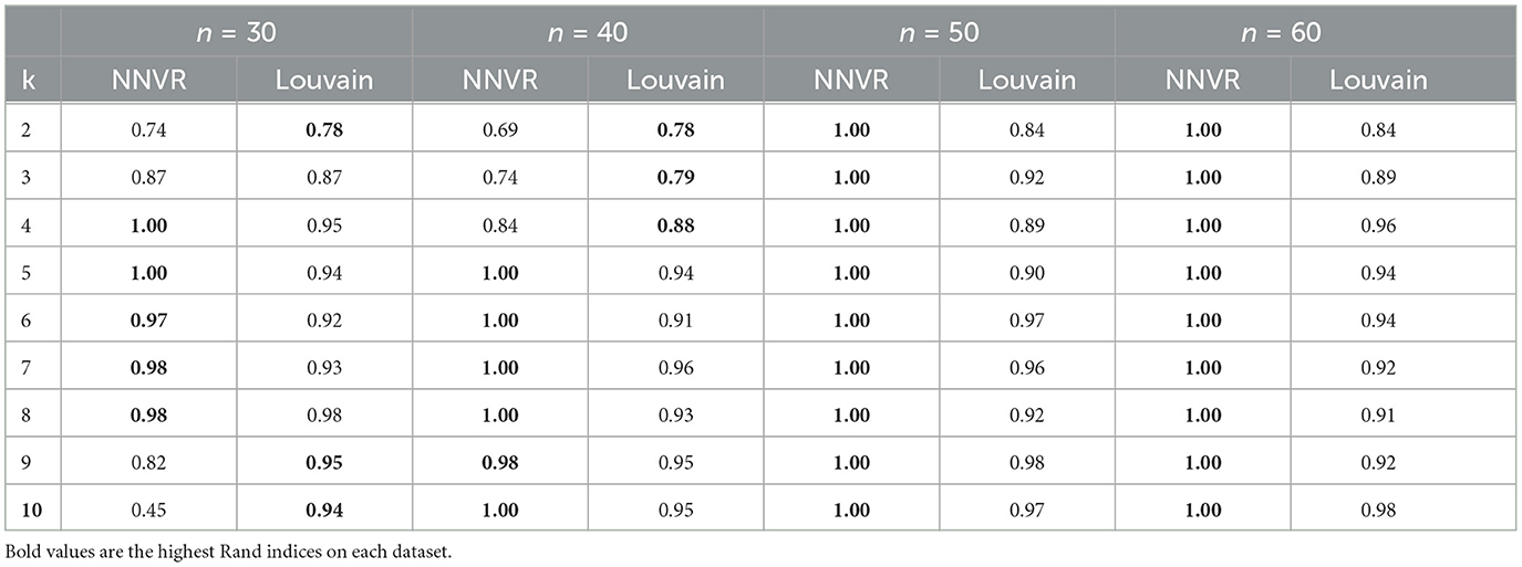
Table 2. Rand indices for n = 30, 40, 50, 60 and k varying from 2 to 10.

5 Conclusion

In this study, we have defined the NNVR filtration, proved its stability, and integrated it in a non-parametric hierarchical clustering algorithm. The NNVR filtration contains more information than the VR filtration, which makes it possible to add an outlier detection step to persistence-based clustering. Our experiments show that our algorithm can perform well despite being fully non-parametric, and can thus be useful in many applications. Future research could explore more advanced methods to choose thresholds on the persistence diagram that could for example select both thresholds simultaneously or incorporate some knowledge depending on the application.

Data availability statement

The original contributions presented in the study are included in the article/Supplementary material, further inquiries can be directed to the corresponding author.

Author contributions

AB: Conceptualization, Data curation, Formal analysis, Investigation, Methodology, Software, Validation, Visualization, Writing – original draft, Writing – review & editing. BT: Supervision, Validation, Writing – review & editing. LO: Supervision, Validation, Writing – review & editing.

Funding

The author(s) declare that no financial support was received for the research, authorship, and/or publication of this article.

Acknowledgments

The authors thank Thibaut Germain for helpful discussions.

Conflict of interest

The authors declare that the research was conducted in the absence of any commercial or financial relationships that could be construed as a potential conflict of interest.

Publisher's note

All claims expressed in this article are solely those of the authors and do not necessarily represent those of their affiliated organizations, or those of the publisher, the editors and the reviewers. Any product that may be evaluated in this article, or claim that may be made by its manufacturer, is not guaranteed or endorsed by the publisher.

Supplementary material

The Supplementary Material for this article can be found online at: https://www.frontiersin.org/articles/10.3389/fams.2024.1260828/full#supplementary-material

Footnotes

1. ^For a review on filtrations over graphs, see [13]. Note that a metric space can be seen as a non-directed weighted graph.

2. ^Here, we define an outlier as an isolated point, and consider that two close points form a cluster.

3. ^In this study, we will simply use the term filtration, as all filtrations considered will be increasing.

4. ^This theorem requires a tameness hypothesis to be verified. Here, it is the case because Proposition 5.1 from [9] applies to the NNVR filtration with the exact same proof as for the VR filtration.

5. ^https://scikit-learn.org/1.2/modules/clustering.html

References

1. Saxena A, Prasad M, Gupta A, Bharill N, Patel OP, Tiwari A, et al. A review of clustering techniques and developments. Neurocomputing. (2017) 267:664–81. doi: 10.1016/j.neucom.2017.06.053

Crossref Full Text | Google Scholar

2. Murtagh F, Contreras P. Algorithms for hierarchical clustering: an overview. Wiley Interdiscipl Rev Data Mining Knowl Discov. (2017) 7:e1219. doi: 10.1002/widm.1219

Crossref Full Text | Google Scholar

3. Ester M, Kriegel HP, Sander J, Xu X. A density-based algorithm for discovering clusters in large spatial databases with noise. KDD. (1996) 96:226–31.

Google Scholar

4. Schubert E, Sander J, Ester M, Kriegel HP, Xu X, DBSCAN. revisited, revisited: why and how you should (still) use DBSCAN. ACM Transact Database Syst. (2017) 42:1–21. doi: 10.1145/3068335

Crossref Full Text | Google Scholar

5. Chazal F, Guibas LJ, Oudot SY, Skraba P. Persistence-based clustering in Riemannian manifolds. J. ACM. (2013) 60:1–38. doi: 10.1145/2535927

Crossref Full Text | Google Scholar

6. Edelsbrunner H, Harer JL. Computational Topology: An Introduction. Providence, RI: American Mathematical Society (2022).

Google Scholar

7. Boissonnat JD, Chazal F, Yvinec M. Geometric and Topological Inference. Vol. 57. Cambridge: Cambridge University Press (2018).

Google Scholar

8. Chazal F, Michel B. An introduction to topological data analysis: fundamental and practical aspects for data scientists. Front Artif Intell. (2021) 4:667963. doi: 10.3389/frai.2021.667963

PubMed Abstract | Crossref Full Text | Google Scholar

9. Chazal F, De Silva V, Oudot S. Persistence stability for geometric complexes. Geometriae Dedicata. (2014) 173:193–214. doi: 10.1007/s10711-013-9937-z

Crossref Full Text | Google Scholar

10. Lee H, Kang H, Chung MK, Kim BN, Lee DS. Persistent brain network homology from the perspective of dendrogram. IEEE Trans Med Imaging. (2012) 31:2267–77. doi: 10.1109/TMI.2012.2219590

PubMed Abstract | Crossref Full Text | Google Scholar

11. Kim H, Hahm J, Lee H, Kang E, Kang H, Lee DS. Brain networks engaged in audiovisual integration during speech perception revealed by persistent homology-based network filtration. Brain Connect. (2015) 5:245–58. doi: 10.1089/brain.2013.0218

PubMed Abstract | Crossref Full Text | Google Scholar

12. Rieck B, Fugacci U, Lukasczyk J, Leitte H. Clique community persistence: a topological visual analysis approach for complex networks. IEEE Trans Vis Comput Graph. (2017) 24:822–31. doi: 10.1109/TVCG.2017.2744321

PubMed Abstract | Crossref Full Text | Google Scholar

13. Aktas ME, Akbas E, Fatmaoui AE. Persistence homology of networks: methods and applications. Appl Netw Sci. (2019) 4:1–28. doi: 10.1007/s41109-019-0179-3

Crossref Full Text | Google Scholar

14. Burago D, Burago Y, Ivanov S. A Course in Metric Geometry. Vol. 33. Providence, RI: American Mathematical Society (2022).

Google Scholar

15. Otsu N. A threshold selection method from gray-level histograms. IEEE Trans Syst Man Cybern. (1979) 9:62–6. doi: 10.1109/TSMC.1979.4310076

Crossref Full Text | Google Scholar

16. Newman ME. Detecting community structure in networks. Eur Phys J B. (2004) 38:321–30. doi: 10.1140/epjb/e2004-00124-y

Crossref Full Text | Google Scholar

17. Rand WM. Objective criteria for the evaluation of clustering methods. J Am Stat Assoc. (1971) 66:846–50. doi: 10.1080/01621459.1971.10482356

Crossref Full Text | Google Scholar

18. Blondel VD, Guillaume JL, Lambiotte R, Lefebvre E. Fast unfolding of communities in large networks. J. Stat. Mech. (2008) 2008:P10008. doi: 10.1088/1742-5468/2008/10/P10008

Crossref Full Text | Google Scholar

19. Hagberg A, Swart PS, Chult D. Exploring Network Structure, Dynamics, and Function Using NetworkX. Los Alamos, NM: Los Alamos National Lab (LANL) (2008).

Google Scholar

20. Arthur D, Vassilvitskii S. K-means++ the advantages of careful seeding. In: Proceedings of the Eighteenth Annual ACM-SIAM Symposium on Discrete Algorithms. Philadelphia, PA: SIAM (2007). p. 1027–35.

Google Scholar

21. Frey BJ, Dueck D. Clustering by passing messages between data points. Science. (2007) 315:972–6. doi: 10.1126/science.1136800

Crossref Full Text | Google Scholar

22. Comaniciu D, Meer P. Mean shift: a robust approach toward feature space analysis. IEEE Trans Pattern Anal Mach Intell. (2002) 24:603–19. doi: 10.1109/34.1000236

Crossref Full Text | Google Scholar

23. Shi. Multiclass spectral clustering. In: Proceedings Ninth IEEE International Conference on Computer Vision. New York, NY: IEEE (2003). p. 313–9.

Google Scholar

24. Nielsen F, Nielsen F. Hierarchical Clustering. Introduction to HPC With MPI for Data Science. New York, NY: Springer (2016). p. 195–211.

Google Scholar

25. Ankerst M, Breunig MM, Kriegel HP, Sander J. Optics: ordering points to identify the clustering structure. ACM Sigmod Record. (1999) 28:49–60. doi: 10.1145/304181.304187

Crossref Full Text | Google Scholar

26. Zhang T, Ramakrishnan R, Livny M. BIRCH: an efficient data clustering method for very large databases. ACM Sigmod Record. (1996) 25:103–14. doi: 10.1145/235968.233324

Crossref Full Text | Google Scholar

27. Moon TK. The expectation-maximization algorithm. IEEE Signal Process Mag. (1996) 13:47–60. doi: 10.1109/79.543975

Crossref Full Text | Google Scholar