Random vector functional link networks for function approximation on manifolds

1 Introduction

In recent years, neural networks have once again triggered an increased interest among researchers in the machine learning community. So-called deep neural networks model functions using a composition of multiple hidden layers, each transforming (possibly non-linearly) the previous layer before building a final output representation [1–5]. In machine learning parlance, these layers are determined by sets of weights and biases that can be tuned so that the network mimics the action of a complex function. In particular, a single layer feed-forward neural network (SLFN) with n nodes may be regarded as a parametric function $f_n:{ℝ}^N\to ℝ$ of the form

$f_n(x)={\displaystyle \sum _{k=1}^n}{v}_k\rho (\langle w_k,x\rangle +b_k),x\in {ℝ}^N.$

Here, the function ρ:ℝ → ℝ is called an activation function and is potentially non-linear. Some typical examples include the sigmoid function $\rho (z)=\frac{1}{1+exp(-z)}$, ReLU ρ(z) = max{0, z}, and sign functions, among many others. The parameters of the SLFN are the number of nodes n ∈ ℕ in the the hidden layer, the input-to-hidden layer weights and biases ${\left\{w_k\right\}}_{k=1}^n\subset {ℝ}^N$ and ${\left\{b_k\right\}}_{k=1}^n\subset ℝ$ (resp.), and the hidden-to-output layer weights ${\left\{v_k\right\}}_{k=1}^n\subset ℝ$. In this way, neural networks are fundamentally parametric families of functions whose parameters may be chosen to approximate a given function.

It has been shown that any compactly supported continuous function can be approximated with any given precision by a single layer neural network with a suitably chosen number of nodes [6], and harmonic analysis techniques have been used to study stability of such approximations [7]. Other recent results that take a different approach directly analyze the capacity of neural networks from a combinatorial point of view [8, 9].

While these results ensure existence of a neural network approximating a function, practical applications require construction of such an approximation. The parameters of the neural network can be chosen using optimization techniques to minimize the difference between the network and the function f:ℝ^N → ℝ it is intended to model. In practice, the function f is usually not known, and we only have access to a set ${\left\{(x_k,f(x_k))\right\}}_{k=1}^m$ of values of the function at finitely many points sampled from its domain, called a training set. The approximation error can be measured by comparing the training data to the corresponding network outputs when evaluated on the same set of points, and the parameters of the neural network f_n can be learned by minimizing a given loss function $\mathcal{L}(x_1,\dots ,x_m)$; a typical loss function is the sum-of-squares error

$\mathcal{L}(x_1,\dots ,x_m)=\frac{1}{m}{\displaystyle \sum _{k=1}^m}|f(x_k)-f_n(x_k){|}^2.$

The SLFN which approximates f is then determined using an optimization algorithm, such as back-propagation, to find the network parameters which minimize $\mathcal{L}(x_1,\dots ,x_m)$. It is known that there exist weights and biases which make the loss function vanish when the number of nodes n is at least m, provided the activation function is bounded, non-linear, and has at least one finite limit at either ±∞ [10].

Unfortunately, optimizing the parameters in SLFNs can be difficult. For instance, any non-linearity in the activation function can cause back-propagation to be very time-consuming or get caught in local minima of the loss function [11]. Moreover, deep neural networks can require massive amounts of training data, and so are typically unreliable for applications with very limited data availability, such as agriculture, healthcare, and ecology [12].

To address some of the difficulties associated with training deep neural networks, both researchers and practitioners have attempted to incorporate randomness in some way. Indeed, randomization-based neural networks that yield closed form solutions typically require less time to train and avoid some of the pitfalls of traditional neural networks trained using back-propagation [11, 13, 14]. One of the popular randomization-based neural network architectures is the Random Vector Functional Link (RVFL) network [15, 16], which is a single layer feed-forward neural network in which the input-to-hidden layer weights and biases are selected randomly and independently from a suitable domain and the remaining hidden-to-output layer weights are learned using training data.

By eliminating the need to optimize the input-to-hidden layer weights and biases, RVFL networks turn supervised learning into a purely linear problem. To see this, define ρ(X) ∈ ℝ^n×m to be the matrix whose jth column is ${\left\{\rho (\langle w_k,x_j\rangle +b_k)\right\}}_{k=1}^n$ and f(X) ∈ ℝ^m the vector whose jth entry is f(x_j). Then, the vector v ∈ ℝⁿ of hidden-to-output layer weights is the solution to the matrix-vector equation f(X) = ρ(X)^Tv, which can be solved by computing the Moore-Penrose pseudoinverse of ρ(X)^T. In fact, there exist weights and biases that make the loss function vanish when the number of nodes n is at least m, provided the activation function is smooth [17].

Although originally considered in the early- to mid-1990s [15, 16, 18, 19], RVFL networks have had much more recent success in several modern applications, including time-series data prediction [20], handwritten word recognition [21], visual tracking [22], signal classification [23, 24], regression [25], and forecasting [26, 27]. Deep neural network architectures based on RVFL networks have also made their way into more recent literature [28, 29], although traditional, single layer RVFL networks tend to perform just as well as, and with lower training costs than, their multi-layer counterparts [29].

Even though RVFL networks are proving their usefulness in practice, the supporting theoretical framework is currently lacking [see 30]. Most theoretical research into the approximation capabilities of deep neural networks centers around two main concepts: universal approximation of functions on compact domains and point-wise approximation on finite training sets [17]. For instance, in the early 1990s, it was shown that multi-layer feed-forward neural networks having activation functions that are continuous, bounded, and non-constant are universal approximators (in the L^p sense for 1 ≤ p < ∞) of continuous functions on compact domains [31, 32]. The most notable result in the existing literature regarding the universal approximation capability of RVFL networks is due to Igelnik and Pao [16] in the mid-1990s, who showed that such neural networks can universally approximate continuous functions on compact sets; the noticeable lack of results since has left a sizable gap between theory and practice. In this study, we begin to bridge this gap by further improving the Igelnik and Pao result, and bringing the mathematical theory behind RFVL networks into the modern spotlight. Below, we introduce the notation that will be used throughout this study, and describe our main contributions.

1.1 Notation

For a function f:ℝ^N → ℝ, the set supp(f)⊂ℝ^N denotes the support of f. We denote by $C_c({ℝ}^N)$ and $C_0({ℝ}^N)$ the classes of continuous functions mapping ℝ^N to ℝ whose support sets are compact and vanish at infinity, respectively. Given a set S⊂ℝ^N, we define its radius to be $\text{rad}(S):={sup}_{x\in S}\parallel x{\parallel }_2$; moreover, if dμ denotes the uniform volume measure on S, then we write $\text{vol}(S):={\int }_S\text{d}\mu$ to represent the volume of S. For any probability distribution P:ℝ^N → [0, 1], a random variable X distributed according to P is denoted by X~P, and we write its expectation as $𝔼X:={\int }_{{ℝ}^N}X\text{d}P$. The open ℓ_p ball of radius r > 0 centered at x ∈ ℝ^N is denoted by $B_p^N(x,r)$ for all 1 ≤ p ≤ ∞; the ℓ_p unit-ball centered at the origin is abbreviated $B_p^N$. Given a fixed δ > 0 and a set S⊂ℝ^N, a minimal δ-net for S, which we denote $\mathcal{C}(\delta ,S)$, is the smallest subset of S satisfying $S\subset {\cup }_{x\in \mathcal{C}(\delta ,S)}{B}_2^N(x,\delta )$; the δ-covering number of S is the cardinality of a minimal δ-net for S and is denoted $\mathcal{N}(\delta ,S):=|\mathcal{C}(\delta ,S)|$.

1.2 Main results

In this study, we analyze the uniform approximation capabilities of RVFL networks. More specifically, we consider the problem of using RVFL networks to estimate a continuous, compactly supported function on N-dimensional Euclidean space.

The first theoretical result on approximating properties of RVFL networks, due to Igelnik and Pao [16], guarantees that continuous functions may be universally approximated on compact sets using RVFL networks, provided the number of nodes n ∈ ℕ in the network goes to infinity. Moreover, it shows that the mean square error of the approximation vanishes at a rate proportional to 1/n. At the time, this result was state-of-the-art and justified how RVFL networks were used in practice. However, the original theorem is not technically correct. In fact, several aspects of the proof technique are flawed. Some of the minor flaws are mentioned in Li et al. [33], but the subsequent revisions do not address the more significant issues which would make the statement of the result technically correct. We address these issues in this study, see Remark 1. Thus, our first contribution to the theory of RVFL networks is a corrected version of the original Igelnik and Pao theorem:

Theorem 1 ([16]). Let $f\in C_c({ℝ}^N)$ with K: = supp(f) and fix any activation function ρ, such that either ρ ∈ L¹(ℝ)∩L^∞(ℝ) with ${\int }_{ℝ}\rho (z)\text{d}z=1$ or ρ is differentiable with ρ′ ∈ L¹(ℝ)∩L^∞(ℝ) and ${\int }_{ℝ}{\rho }^{\prime }(z)\text{d}z=1$. For any ε > 0, there exist distributions from which input weights ${\left\{w_k\right\}}_{k=1}^n$ and biases ${\left\{b_k\right\}}_{k=1}^n$ are drawn, and there exist hidden-to-output layer weights ${\left\{v_k\right\}}_{k=1}^n\subset ℝ$ that depend on the realization of weights and biases, such that the sequence of RVFL networks ${\left\{f_n\right\}}_{n=1}^{\infty }$ is defined by

$f_n(x):={\displaystyle \sum _{k=1}^n}{v}_k\rho (\langle w_k,x\rangle +b_k)\text{for}x\in K$

satisfies

$𝔼{\displaystyle {\int }_K}|f(x)-f_n(x){|}^2\text{d}x<\epsilon +O(1/n),$

as n → ∞.

For a more precise formulation of Theorem 1 and its proof, we refer the reader to Theorem 5 and Section 3.1.

Remark 1.

1. Even though in Theorem 1 we only claim existence of the distribution for input weights ${\left\{w_k\right\}}_{k=1}^n$ and biases ${\left\{b_k\right\}}_{k=1}^n$, such a distribution is actually constructed in the proof. Namely, for any ε > 0, there exist constants α, Ω > 0 such that the random variables

$\begin{array}{l}{w}_k~\text{Unif }({[-\alpha \Omega ,\alpha \Omega ]}^N);\\ y_k~\text{Unif }(K);\\ u_k~\text{Unif }([-\frac{\pi }{2}(2L+1),\frac{\pi }{2}(2L+1)]),\\ \text{ where }L:\text{= }\lceil \frac{\text{2N}}{\pi }\text{rad}(K)\Omega -\frac{1}{2}\rceil ,\end{array}$

are independently drawn from their associated distributions, and b_k: = −〈w_k, y_k〉 −αu_k.

2. We note that, unlike the original theorem statement in Igelnik and Pao [16], Theorem 1 does not show exact convergence of the sequence of constructed RVFL networks f_n to the original function f. Indeed, it only ensures that the limit f_n is ε-close to f. This should still be sufficient for practical applications since, given a desired accuracy level ε > 0, one can find values of α, Ω, andn such that this accuracy level is achieved on average. Exact convergence can be proved if one replaces α and Ω in the distribution described above by sequences ${\left\{{\alpha }_n\right\}}_{n=1}^{\infty }$ and ${\left\{{\Omega }_n\right\}}_{n=1}^{\infty }$ of positive numbers, both tending to infinity with n. In this setting, however, there is no guaranteed rate of convergence; moreover, as n increases, the ranges of the random variables ${\left\{w_k\right\}}_{k=1}^n$ and ${\left\{u_k\right\}}_{k=1}^n$ become increasingly larger, which may cause problems in practical applications.

3. The approach we take to construct the RVFL network approximating a function f allows one to compute the output weights ${\left\{v_k\right\}}_{k=1}^n$ exactly (once the realization of random parameters is fixed), in the case where the function f is known. For the details, we refer the reader to Equations 6, 8 in the proof of Theorem 1. If we only have access to a training set that is sufficiently large and uniformly distributed over the support of f, these formulas can be used to compute the output weights approximately, instead of solving the least squares problem.

4. Note that the normalization ${\int }_{ℝ}\rho (z)\text{d}z=1$ of the activation function can be replaced by the condition ${\int }_{ℝ}\rho (z)\text{d}z\ne 0$. Indeed, in the case when ρ ∈ L¹(ℝ)∩L^∞(ℝ) and ${\int }_{ℝ}\rho (z)\text{d}z\notin \left\{0,1\right\},$ one can simply use Theorem 1 to approximate $\frac{1}{{\int }_{ℝ}\rho (z)\text{d}z}f$ by a sequence of RVFL network with the activation function $\frac{1}{{\int }_{ℝ}\rho (z)\text{d}z}\rho$. Mutatis mutandis in the case when ${\int }_{ℝ}{\rho }^{\prime }(z)\text{d}{z}^{\prime }\notin \left\{0,1\right\}.$ More generally, this trick allows any of our theorems to be applied in the case ${\int }_{ℝ}\rho (z)\text{d}z\ne 0.$

One of the drawbacks of Theorem 1 is that the mean square error guarantee is asymptotic in the number of nodes used in the neural network. This is clearly impractical for applications, and so it is desirable to have a more explicit error bound for each fixed number n of nodes used. To this end, we provide a new, non-asymptotic version of Theorem 1, which provides an error guarantee with high probability whenever the number of network nodes is large enough, albeit at the price of an additional Lipschitz requirement on the activation function:

Theorem 2 Let $f\in C_c({ℝ}^N)$ with K: = supp(f) and fix any activation function ρ ∈ L¹(ℝ)∩L^∞(ℝ) with ${\int }_{ℝ}\rho (z)\text{d}z=1.$ Suppose further that ρ is κ-Lipschitz on ℝ for some κ > 0. For any ε > 0 and η ∈ (0, 1), suppose that n ≥ C(N, f, ρ)ε⁻¹log(η⁻¹/ε), where C(N, f, ρ) is independent of ε and η and depends on f, ρ, and superexponentially on N. Then, there exist distributions from which input weights ${\left\{w_k\right\}}_{k=1}^n$ and biases ${\left\{b_k\right\}}_{k=1}^n$ are drawn, and there exist hidden-to-output layer weights ${\left\{v_k\right\}}_{k=1}^n\subset ℝ$ that depend on the realization of weights and biases, such that the RVFL network defined by

$f_n(x):={\displaystyle \sum _{k=1}^n}{v}_k\rho (\langle w_k,x\rangle +b_k)\text{for}x\in K$

satisfies

${\displaystyle {\int }_K}|f(x)-f_n(x){|}^2\text{d}x<\epsilon$

with probability at least 1−η.

For simplicity, the bound on the number n of the nodes on the hidden layer here is rough. For a more precise formulation of this result that contains a bound with explicit constant, we refer the reader to Theorem 6 in Section 3.2. We also note that the distribution of the input weight and bias here can be selected as described in Remark 1.

The constructions of RVFL networks presented in Theorems 1, 2 depend heavily on the dimension of the ambient space ℝ^N. If N is small, this dependence does not present much of a problem. However, many modern applications require the ambient dimension to be large. Fortunately, a common assumption in practice is the support of the signals of interest lies on a lower-dimensional manifold embedded in ℝ^N. For instance, the landscape of cancer cell states can be modeled using non-linear, locally continuous “cellular manifolds;” indeed, while the ambient dimension of this state space is typically high (e.g., single-cell RNA sequencing must account for approximately 20,000 gene dimensions), cellular data actually occupies an intrinsically lower dimensional space [34]. Similarly, while the pattern space of neural population activity in the brain is described by an exponential number of parameters, the spatiotemporal dynamics of brain activity lie on a lower-dimensional subspace or “neural manifold” [35]. In this study, we propose a new RVFL network architecture for approximating continuous functions defined on smooth compact manifolds that allows to replace the dependence on the ambient dimension N with dependence on the manifold intrinsic dimension. We show that RVFL approximation results can be extended to this setting. More precisely, we prove the following analog of Theorem 2.

Theorem 3 Let $\mathcal{M}\subset {ℝ}^N$ be a smooth, compact d-dimensional manifold with finite atlas {(_{Uj, ϕj)}j ∈ J} and $f\in C(\mathcal{M})$. Fix any activation function ρ ∈ L¹(ℝ)∩L^∞(ℝ) with ${\int }_{ℝ}\rho (z)\text{d}z=1$ such that ρ is κ-Lipschitz on ℝ for some κ > 0. For any ε > 0 and η ∈ (0, 1), suppose n ≥ C(d, f, ρ)ε⁻¹log(η⁻¹/ε), where C(d, f, ρ) is independent of ε and η and depends on f, ρ, and superexponentially on d. Then, there exists an RVFL-like approximation f_n of the function f with a parameter selection similar to the Theorem 1 construction that satisfies

${\displaystyle {\int }_{\mathcal{M}}}|f(x)-f_n(x){|}^2\text{d}x<\epsilon$

with probability at least 1−η.

For a the construction of the RVFL-like approximation f_n and a more precise formulation of this result and an analog of Theorem 1 applied to manifolds, we refer the reader to Section 3.3.1 and Theorems 7, 8. We note that the approximation f_n here is not obtained as a single RVFL network construction, but rather as a combination of several RVFL networks in local manifold coordinates.

1.3 Organization

The remaining part of the article is organized as follows. In Section 2, we discuss some theoretical preliminaries on concentration bounds for Monte-Carlo integration and on smooth compact manifolds. Monte-Carlo integration is an essential ingredient in our construction of RVFL networks approximating a given function, and we use the results listed in this section to establish approximation error bounds. Theorem 1 is proven in Section 3.1, where we break down the proof into four main steps, constructing a limit-integral representation of the function to be approximated in Lemmas 3, 4, then using Monte-Carlo approximation of the obtained integral to construct an RVFL network in Lemma 5, and, finally, establishing approximation guarantees for the constructed RVFL network. The proofs of Lemmas 3, 4, and 5 can be found in Sections 3.5.1, 3.5.2, and 3.5.3, respectively. We further study properties of the constructed RVFL networks and prove the non-asymptotic approximation result of Theorem 2 in Section 3.2. In Section 3.3, we generalize our results and propose a new RVFL network architecture for approximating continuous functions defined on smooth compact manifolds. We show that RVFL approximation results can be extended to this setting by proving an analog of Theorem 1 in Section 3.3.2 and Theorem 3 in Section 3.5.5. Finally, in Section 3.4, we provide numerical evidence to illustrate the result of Theorem 3.

2 Materials and methods

In this section, we briefly introduce supporting material and theoretical results which we will need in later sections. This material is far from exhaustive, and is meant to be a survey of definitions, concepts, and key results.

2.1 A concentration bound for classic Monte-Carlo integration

A crucial piece of the proof technique employed in Igelnik and Pao [16], which we will use repeatedly, is the use of the Monte-Carlo method to approximate high-dimensional integrals. As such, we start with the background on Monte-Carlo integration. The following introduction is adapted from the material in Dick et al. [36].

Let f:ℝ^N → ℝ and S⊂ℝ^N a compact set. Suppose we want to estimate the integral $I(f,S):={\int }_{S}f\text{d}\mu$, where μ is the uniform measure on S. The classic Monte Carlo method does this by an equal-weight cubature rule,

$I_n(f,S):=\frac{\text{vol}(S)}{n}{\displaystyle \sum _{j=1}^n}f(x_j),$

where ${\left\{x_j\right\}}_{j=1}^n$ are independent identically distributed uniform random samples from S and $\text{vol}(S):={\int }_{S}d\mu$ is the volume of S. In particular, note that 𝔼I_n(f, S) = I(f, S) and

$𝔼I_n{(f,S)}^2=\frac{1}{n}\text{vol}(S)I(f^2,S)+(n-1)I{(f,S)}^2.$

Let us define the quantity

$\begin{array}{ll}\sigma {(f,S)}^2:=\frac{I(f^2,S)}{\text{vol}(S)}-\frac{I{(f,S)}^2}{\text{vo}{\text{l}}^2(S)}.& (1)\end{array}$

It follows that the random variable I_n(f) has mean I(f, S) and variance vol²(S)σ(f, S)²/n. Hence, by the Central Limit Theorem, provided that 0 < vol²(S)σ(f, S)² < ∞, we have

$\underset{n\to \infty }{\lim }\mathbb{P}\left(|I_n(f,S)-I(f,S)|\le \frac{C\epsilon (f,S)}{\sqrt{n}}\right)={(2\pi )}^{-1/2}{\displaystyle {\int }_{-C}^C{e}^{-x^2/2}dx}$

for any constant C > 0, where ε(f, S): = vol(S)σ(f, S). This yields the following well-known result:

Theorem 4 For any f ∈ L²(S, μ), the mean-square error of the Monte Carlo approximation I_n(f, S) satisfies

$𝔼{|I}_n(f,S)-I(f,S)|{}^2=\frac{\text{vo}{\text{l}}^2(S)\sigma {(f,S)}^2}{n},$

where the expectation is taken with respect to the random variables ${\left\{x_j\right\}}_{j=1}^n$ and σ(f, S) is defined in Equation 1.

In particular, Theorem 4 implies $𝔼I_n(f,S)-I(f,S){}^2=O(1/n)$ as n → ∞.

In the non-asymptotic setting, we are interested in obtaining a useful bound on the probability ℙ(|I_n(f, S)−I(f, S)| ≥ t) for all t > 0. The following lemma follows from a generalization of Bennett's inequality (Theorem 7.6 in [37]; see also [38, 39]).

Lemma 1 For any f ∈ L²(S) and n ∈ ℕ, we have

$\mathbb{P}(|I_n(f,S)-I(f,S)|\ge t)\le 3exp\left(-\frac{nt}{CK}log\left(1+\frac{Kt}{\text{vol}(S)I(f^2,S)}\right)\right)$

for all t > 0 and a universal constant C > 0, provided |vol(S)f(x)| ≤ K for almost every x ∈ S.

2.2 Smooth, compact manifolds in Euclidean space

In this section, we review several concepts of smooth manifolds that will be useful to us later. Many of the definitions and results that follow can be found, for instance, in Shaham et al. [40]. Let $\mathcal{M}\subset {ℝ}^N$ be a smooth, compact d-dimensional manifold. A chart for $\mathcal{M}$ is a pair (U, ϕ) such that $U\subset \mathcal{M}$ is an open set and ϕ:U → ℝ^d is a homeomorphism. One way to interpret a chart is as a tangent space at some point x ∈ U; in this way, a chart defines a Euclidean coordinate system on U via the map ϕ. A collection {(_{Uj, ϕj)}j ∈ J} of charts defines an atlas for $\mathcal{M}$ if ${\cup }_{j\in J}{U}_j=\mathcal{M}$. We now define a special collection of functions on $\mathcal{M}$ called a partition of unity.

Definition 1 Let $\mathcal{M}\subset {ℝ}^N$ be a smooth manifold. A partition of unity of $\mathcal{M}$ with respect to an open cover {_{Uj}j ∈ J} of $\mathcal{M}$ is a family of non-negative smooth functions {_{ηj}j ∈ J} such that for every $x\in \mathcal{M}$, we have $1=\sum _{j\in J}{\eta }_j(x)$ and, for every j ∈ J, supp(η_j)⊂U_j.

It is known that if $\mathcal{M}$ is compact, there exists a partition of unity of $\mathcal{M}$ such that supp(η_j) is compact for all j ∈ J [see 41]. In particular, such a partition of unity exists for any open cover of $\mathcal{M}$ corresponding to an atlas.

Fix an atlas {(_{Uj, ϕj)}j ∈ J} for $\mathcal{M}$, as well as the corresponding, compactly supported partition of unity {_{ηj}j ∈ J}. Then, we have the following useful result [see 40, Lemma 4.8].

Lemma 2 Let $\mathcal{M}\subset {ℝ}^N$ be a smooth, compact manifold with atlas {(_{Uj, ϕj)}j ∈ J} and compactly supported partition of unity {_{ηj}j ∈ J}. For any $f\in C(\mathcal{M})$, we have

$f(x)={\displaystyle \sum _{\left\{j\in J:x\in U_j\right\}}}({\widehat{f}}_j◦{\varphi }_j)(x)$

for all $x\in \mathcal{M}$, where

${\widehat{f}}_j(z):=\{\begin{array}{ll}f({\varphi }_j^{-1}(z)){\eta }_j({\varphi }_j^{-1}(z))\hfill & z\in {\varphi }_j(U_j)\hfill \\ 0\hfill & \text{otherwise}.\hfill \end{array}$

In later sections, we use the representation of Lemma 2 to integrate functions $f\in C(\mathcal{M})$ over $\mathcal{M}$. To this end, for each j ∈ J, let Dϕ_j(y) denote the differential of ϕ_j at y ∈ U_j, which is a map from the tangent space $T_y\mathcal{M}$ into ℝ^d. One may interpret Dϕ_j(y) as the matrix representation of a basis for the cotangent space at y ∈ U_j. As a result, Dϕ_j(y) is necessarily invertible for each y ∈ U_j, and so we know that |det(Dϕ_j(y))| > 0 for each y ∈ U_j. Hence, it follows by the change of variables theorem that

$\begin{array}{l}{\displaystyle {\int }_{ℳ}f}(x)\text{d}x={\displaystyle {\int }_{ℳ}{\displaystyle \sum _{\{j\in J:x\in U_j\}}({\widehat{f}}_j°{\varphi }_j)(x)}}\text{d}x\\ ={\displaystyle \sum _{j\in J}{\displaystyle {\int }_{{\varphi }_j(U_j)}\frac{{\widehat{f}}_j(z)}{|\det (D{\varphi }_j({\varphi }_j^{-1}(z)))|}}}\text{d}z.& (2)\end{array}$

3 Results

In this section, we prove our main results formulated in Section 1.2 and also use numerical simulations to illustrate the RVFL approximation performance in a low-dimensional submanifold setup. To improve readability of this section, we postpone the proofs of technical lemmas till Section 3.5.

3.1 Proof of Theorem 1

We split the proof of the theorem into two parts, first handling the case ρ ∈ L¹(ℝ)∩L^∞(ℝ) and second, addressing the case ρ′ ∈ L¹(ℝ)∩L^∞(ℝ).

3.1.1 Proof of Theorem 1 when ρ ∈ L¹(ℝ)∩L^∞(ℝ)

We begin by restating the theorem in a form that explicitly includes the distributions that we draw our random variables from.

Theorem 5 ([16]) Let $f\in C_c({ℝ}^N)$ with K: = supp(f) and fix any activation function ρ ∈ L¹(ℝ)∩L^∞(ℝ) with ${\int }_{ℝ}\rho (z)\text{d}z=1$. For any ε > 0, there exist constants α, Ω > 0 such that the following holds: If, for k ∈ ℕ, the random variables

$\begin{array}{l}{w}_k~\text{Unif }({[-\alpha \Omega ,\alpha \Omega ]}^N);\\ y_k~\text{Unif }(K);\\ u_k~\text{Unif }([-\frac{\pi }{2}(2L+1),\frac{\pi }{2}(2L+1)]),\\ \text{ where }L:\text{=}\lceil \frac{\text{2N}}{\pi }\text{rad}(K)\Omega -\frac{1}{2}\rceil ,\end{array}$

are independently drawn from their associated distributions, and

$b_k:=-\langle w_k,y_k\rangle -\alpha u_k,$

then there exist hidden-to-output layer weights ${\left\{v_k\right\}}_{k=1}^n\subset ℝ$ (that depend on the realization of the weights ${\left\{w_k\right\}}_{k=1}^n$ and biases ${\left\{b_k\right\}}_{k=1}^n$) such that the sequence of RVFL networks ${\left\{f_n\right\}}_{n=1}^{\infty }$ defined by

$f_n(x):={\displaystyle \sum _{k=1}^n}{v}_k\rho (\langle w_k,x\rangle +b_k)\text{for}x\in K$

satisfies

$𝔼{\displaystyle {\int }_K}|f(x)-f_n(x){|}^2\text{d}x\le \epsilon +O(1/n).$

as n → ∞.

Proof. Our proof technique is based on that introduced by Igelnik and Pao and can be divided into four steps. The first three steps essentially consist of Lemma 3, Lemma 4, and Lemma 5, and the final step combines them to obtain the desired result. First, the function f is approximated by a convolution, given in Lemma 3. The proof of this result can be found in Section 3.5.1.

Lemma 3 Let $f\in C_0({ℝ}^N)$ and h ∈ L¹(ℝ^N) with ${\int }_{{ℝ}^N}h(z)\text{d}z=1.$ For Ω > 0, define

$\begin{array}{ll}{h}_{\Omega }(y):={\Omega }^{N}h(\Omega y).& (3)\end{array}$

Then, we have

$\begin{array}{ll}f(x)={\displaystyle \underset{\Omega \to \infty }{lim}}(f*h_{\Omega })(x)& (4)\end{array}$

uniformly for all x ∈ ℝ^N.

Next, we represent f as the limiting value of a multidimensional integral over the parameter space. In particular, we replace (f*h_Ω)(x) in the convolution identity (Equation 4) with a function of the form ${\int }_{K}F(y)\rho (\langle w,x\rangle +b(y))\text{d}y$, as this will introduce the RVFL structure we require. To achieve this, we first use a truncated cosine function in place of the activation function ρ and then switch back to a general activation function.

To that end, for each fixed Ω > 0, let $L=L(\Omega ):=\lceil \frac{2N}{\pi }\text{rad}(K)\Omega -\frac{1}{2}\rceil$ and define cos_Ω:ℝ → [−1, 1] by

$\begin{array}{ll}{\cos }_{\Omega }(x):=\{\begin{array}{ll}\cos (x)\hfill & x\in [-\frac{1}{2}(2L+1)\pi ,\frac{1}{2}(2L+1)\pi ],\hfill \\ 0\hfill & \text{otherwise}.\hfill \end{array}& (5)\end{array}$

Moreover, introduce the functions

$\begin{array}{l}{F}_{\alpha ,\Omega }(y,w,u):=\frac{\alpha }{{(2\pi )}^N}f(y){\cos }_{\Omega }(u){\displaystyle \prod _{j=1}^N\varphi }(w(j)/\Omega ),\\ b_{\alpha }(y,w,u):=-\alpha (\langle w,y\rangle +u)& (6)\end{array}$

where y, w ∈ ℝ^N, u ∈ ℝ, and ϕ = A*A for any even function A ∈ C^∞(ℝ) supported on $\left[-\frac{1}{2},\frac{1}{2}\right]$ s.t. ∥A∥₂ = 1. Then, we have the following lemma, a detailed proof of which can be found in Section 3.5.2.

Lemma 4 Let $f\in C_c({ℝ}^N)$ and ρ ∈ L¹(ℝ) with K: = supp(f) and ${\int }_{ℝ}\rho (z)\text{d}z=1$. Define F_{α, Ω} and b_α as in Equation 6 for all α > 0. Then, for $L:=\lceil \frac{2N}{\pi }\text{rad}(K)\Omega -\frac{1}{2}\rceil$, we have

$\begin{array}{ll}f(x)={\displaystyle \underset{\Omega \to \infty }{lim}}{\displaystyle \underset{\alpha \to \infty }{lim}}{\displaystyle {\int }_{K(\Omega )}}{F}_{\alpha ,\Omega }(y,w,u)\rho (\alpha \langle w,x\rangle +b_{\alpha }(y,w,u))\text{d}y\text{d}w\text{d}u& (7)\end{array}$

uniformly for every x ∈ K, where $K(\Omega ):=K\times {\left[-\Omega ,\Omega \right]}^N\times \left[-\frac{\pi }{2}(2L+1),\frac{\pi }{2}(2L+1)\right]$.

The next step in the proof of Theorem 5 is to approximate the integral in Equation 7 using the Monte-Carlo method. Define $v_k:=\frac{\text{vol}(K(\Omega ))}{n}{F}_{\alpha ,\Omega }{y}_k,\frac{w_k}{\alpha },u_k$ for k = 1, …, n, and the random variables ${\left\{f_n\right\}}_{n=1}^{\infty }$ by

$\begin{array}{ll}{f}_n(x):={\displaystyle \sum _{k=1}^n}{v}_k\rho (\langle w_k,x\rangle +b_k).& (8)\end{array}$

Then, we have the following lemma that is proven in Section 3.5.3.

Lemma 5 Let $f\in C_c({ℝ}^N)$ and ρ ∈ L¹(ℝ)∩L^∞(ℝ) with K: = supp(f) and ${\int }_{ℝ}\rho (z)\text{d}z=1$. Then, as n → ∞, we have

$\begin{array}{l}𝔼{\displaystyle {\int }_K|{\displaystyle {\int }_{K(\Omega )}{F}_{\alpha ,\Omega }}(y,w,u)\rho (\alpha \langle w,x\rangle +b_{\alpha }(y,w,u))\text{d}y\text{d}w\text{d}u}\\ {-f_n(x)|}^2\text{d}x=O(1/n),& (9)\end{array}$

where $K(\Omega ):=K\times {\left[-\Omega ,\Omega \right]}^N\times \left[-\frac{\pi }{2}(2L+1),\frac{\pi }{2}(2L+1)\right]$ and $L:=\lceil \frac{2N}{\pi }\text{rad}(K)\Omega -\frac{1}{2}\rceil$.

To complete the proof of Theorem 5, we combine the limit representation (Equation 7) with the Monte-Carlo error guarantee (Equation 9) and show that, given any ε > 0, there exist α, Ω > 0 such that

$𝔼{\displaystyle {\int }_K}|f(x)-f_n(x){|}^2\text{d}x\le \epsilon +O(1/n)$

as n → ∞. To this end, let ε′ > 0 be arbitrary and consider the integral I(x; p) given by

$\begin{array}{ll}I(x;p):={\displaystyle {\int }_{K(\Omega )}}{(F}_{\alpha ,\Omega }(y,w,u)\rho (\alpha \langle w,x\rangle +b_{\alpha }(y,w,u))){}^p\text{d}y\text{d}w\text{d}u& (10)\end{array}$

for x ∈ K and p ∈ ℕ. By Equation 7, there exist α, Ω > 0 such that |f(x)−I(x; 1)| < ε′ holds for every x ∈ K, and so it follows that

$|f(x)-f_n(x)|<{\epsilon }^{\prime }+|I(x;1)-f_n(x)|$

for every x ∈ K. Jensen's inequality now yields that

$\begin{array}{ll}𝔼{\displaystyle {\int }_K}|f(x)-f_n(x){|}^2\text{d}x\le 2\text{vol}(K){({\epsilon }^{\prime })}^2+2𝔼{\displaystyle {\int }_K}I(x;1)-f_n(x){}^2\text{d}x.& (11)\end{array}$

By Equation 9, we know that the second term on the right-hand side of Equation 11 is O(1/n). Therefore, we have

$𝔼{\displaystyle {\int }_K}|f(x)-f_n(x){|}^2\text{d}x\le 2\text{vol}(K){({\epsilon }^{\prime })}^2+O(1/n),$

and so the proof is completed by taking ${\epsilon }^{\prime }=\sqrt{\epsilon /2\text{vol}(K)}$ and choosing α, Ω > 0 accordingly.

3.1.2 Proof of Theorem 1 when ρ′ ∈ L¹(ℝ)∩L^∞(ℝ)

The full statement of the theorem is identical to that of Theorem 5 albeit now with ρ′ ∈ L¹(ℝ)∩L^∞(ℝ), so we omit it for brevity. Its proof is also similar to the proof of the case where ρ ∈ L¹(ℝ)∩L^∞(ℝ) with some key modifications. Namely, one uses an integration by parts argument to modify the part of the proof corresponding to Lemma 4. The details of this argument are presented in Section 3.5.4.

3.2 Proof of Theorem 2

In this section, we prove the non-asymptotic result for RVFL networks in ℝ^N, and we begin with a more precise statement of the theorem that makes all the dimensional dependencies explicit.

Theorem 6 Consider the hypotheses of Theorem 5 and suppose further that ρ is κ-Lipschitz on ℝ for some κ > 0. For any

$0<\delta <\frac{\sqrt{\epsilon }}{8\sqrt{2N}\kappa {\alpha }^{2}M\Omega {(\Omega /\pi )}^N\text{vo}{\text{l}}^{3/2}(K)(\pi +2N\text{rad}(K)\Omega )},$

suppose

$n\ge \frac{c\Sigma \alpha {(\Omega /\pi )}^N(\pi +2N\text{rad}(K)\Omega )log(3{\eta }^{-1}\mathcal{N}(\delta ,K))}{\sqrt{\epsilon }log(1+\frac{\sqrt{\epsilon }}{\Sigma \alpha {(\Omega /\pi )}^N(\pi +2N\text{rad}(K)\Omega )})},$

where $M:=\underset{x\in K}{sup}|f(x)|$, c > 0 is a numerical constant, and Σ is a constant depending on f and ρ, and let parameters ${\left\{w_k\right\}}_{k=1}^n$, ${\left\{b_k\right\}}_{k=1}^n$, and ${\left\{v_k\right\}}_{k=1}^n$ be as in Theorem 5. Then, the RVFL network defined by

$f_n(x):={\displaystyle \sum _{k=1}^n}{v}_k\rho (\langle w_k,x\rangle +b_k)\text{for}x\in K$

satisfies

${\displaystyle {\int }_K}|f(x)-f_n(x){|}^2\text{d}x<\epsilon$

with probability at least 1−η.

Proof. Let $f\in C_c({ℝ}^N)$ with K: = supp(f) and suppose ε > 0, η ∈ (0, 1) are fixed. Take an arbitrarily κ-Lipschitz activation function ρ ∈ L¹(ℝ)∩L^∞(ℝ). We wish to show that there exists an RVFL network ${\left\{f_n\right\}}_{n=1}^{\infty }$ defined on K that satisfies the

${\displaystyle {\int }_K}|f(x)-f_n(x){|}^2\text{d}x<\epsilon$

with probability at least 1−η when n is chosen sufficiently large. The proof is obtained by modifying the proof of Theorem 5 for the asymptotic case.

We begin by repeating the first two steps in the proof of Theorem 5 from Sections 3.5.1, 3.5.2. In particular, by Lemma 4 we have the representation given by Equation 4, namely,

$f(x)={\displaystyle \underset{\Omega \to \infty }{lim}}{\displaystyle \underset{\alpha \to \infty }{lim}}{\displaystyle {\int }_{K(\Omega )}}{F}_{\alpha ,\Omega }(y,w,u)\rho (\alpha \langle w,x\rangle +b_{\alpha }(y,w,u))\text{d}y\text{d}w\text{d}u$

holds uniformly for all x ∈ K. Hence, if we define the random variables f_n and I_n from Section 3.5.3 as in Equations 8, 29, respectively, we seek a uniform bound on the quantity

$|f(x)-f_n(x)|\le |f(x)-I(x;1)|+|I_n(x)-I(x;1)|$

over the compact set K, where I(x; 1) is given by Equation 10 for all x ∈ K. Since Equation 7 allows us to fix α, Ω > 0 such that

$\begin{array}{l}|f(x)-I(x;1)|=|f(x)-\\ {\displaystyle {\int }_{K(\Omega )}{F}_{\alpha ,\Omega }}(y,w,u)\rho (\alpha \langle w,x\rangle +b_{\alpha }(y,w,u))\text{d}y\text{d}w\text{d}u|<\sqrt{\frac{\epsilon }{2\text{vol}(K)}}\end{array}$

holds for every x ∈ K simultaneously, the result would follow if we show that, with high probability, $|I_n(x)-I(x;1)|<\sqrt{\epsilon /2\text{vol}(K)}$ uniformly for all x ∈ K. Indeed, this would yield

$\begin{array}{l}{\displaystyle {\int }_K|}f(x)-f_n(x){|}^2\text{d}x\le 2{\displaystyle {\int }_K|}f(x)-I(x;1){|}^2\text{d}x\\ +2{\displaystyle {\int }_K|}{I}_n(x)-I(x;1){|}^2\text{d}x<\epsilon \end{array}$

with high probability. To this end, for δ > 0, let $\mathcal{C}(\delta ,K)\subset K$ denote a minimal δ-net for K, with cardinality $\mathcal{N}(\delta ,K)$. Now, fix x ∈ K and consider the inequality

$\begin{array}{l}|I_n(x)-I(x;1)|\le \underset{(*)}{\underbrace{|I_n(x)-I_n(z)|}}+\underset{(**)}{\underbrace{|I_n(z)-I(z;1)|}}\\ +\underset{(***)}{\underbrace{|I(x;1)-I(z;1)|}},& (12)\end{array}$

where $z\in \mathcal{C}(\delta ,K)$ is such that ∥x−z∥₂ < δ. We will obtain the desired bound on Equation 12 by bounding each of the terms (*), (**), and (***) separately.

First, we consider the term (*). Recalling the definition of I_n, observe that we have

$\begin{array}{l}(*)=\frac{\text{vol}(K(\Omega ))}{n}|{\displaystyle \sum _{k=1}^n{F}_{\alpha ,\Omega }}(y_k,w_k,u_k)(\rho (\alpha \langle w_k,x\rangle +b_{\alpha }(y_k,w_k,u_k))\\ -\rho (\alpha \langle w_k,z\rangle +b_{\alpha }(y_k,w_k,u_k)))|\\ \le \frac{\alpha M\text{vol}(K(\Omega ))}{{(2\pi )}^{N}n}{\displaystyle \sum _{k=1}^n|}\rho (\alpha \langle w_k,x\rangle +b_{\alpha }(y_k,w_k,u_k))\\ -\rho (\alpha \langle w_k,z\rangle +b_{\alpha }(y_k,w_k,u_k))|\\ \le \alpha M{(2\pi )}^{-N}\text{vol}(K(\Omega ))R_{\alpha ,\Omega }(x,z),\end{array}$

where $M:=\underset{x\in K}{sup}|f(x)|$ and we define

$\begin{array}{l}{R}_{\alpha ,\Omega }(x,z):=\underset{\begin{array}{c}y\in K\\ w\in {[-\Omega ,\Omega ]}^N\\ u\in [-(L+\frac{1}{2})\pi ,(L+\frac{1}{2})\pi ]\end{array}}{\sup }|\rho (\alpha \langle w,x\rangle +b_{\alpha }(y,w,u))\\ -\rho (\alpha \langle w,z\rangle +b_{\alpha }(y,w,u))|.\end{array}$

Now, since ρ is assumed to be κ-Lipschitz, we have

$\begin{array}{l}|\rho (\alpha \langle w,x\rangle +b_{\alpha }(y,w,u))-\rho (\alpha \langle w,z\rangle +b_{\alpha }(y,w,u))|\\ =|\rho (\alpha (\langle w,x-y\rangle -u))\\ -\rho (\alpha (\langle w,z-y\rangle -u))|\le \kappa \alpha |\langle w,x-z\rangle |\end{array}$

for any y ∈ K, w ∈ [−Ω, Ω]^N, and $u\in \left[-(L+\frac{1}{2})\pi ,(L+\frac{1}{2})\pi \right].$ Hence, an application of the Cauchy–Schwarz inequality yields $R_{\alpha ,\Omega }(x,z)\le \kappa \alpha \Omega \delta \sqrt{N}$ for all x ∈ K, from which it follows that

$\begin{array}{ll}(*)\le M\sqrt{N}\kappa \delta {\alpha }^2\Omega {(2\pi )}^{-N}\text{vol}(K(\Omega ))& (13)\end{array}$

holds for all x ∈ K.

Next, we bound (***) using a similar approach. Indeed, by the definition of I(·;1), we have

$\begin{array}{l}(***)=|{\displaystyle {\int }_{K(\Omega )}{F}_{\alpha ,\Omega }}(y,w,u)(\rho (\alpha \langle w,x\rangle +b_{\alpha }(y,w,u))\\ -\rho (\alpha \langle w,z\rangle +b_{\alpha }(y,w,u)))\text{d}y\text{d}w\text{d}u|\\ \le \frac{\alpha M\Vert \varphi {\Vert }_{\infty }^N}{{(2\pi )}^N}{\displaystyle {\int }_{K(\Omega )}|}\rho (\alpha \langle w,x\rangle +b_{\alpha }(y,w,u))\\ -\rho (\alpha \langle w,z\rangle +b_{\alpha }(y,w,u))|\text{d}y\text{d}w\text{d}u\\ \le \alpha M{(2\pi )}^{-N}\text{vol}(K(\Omega ))R_{\alpha ,\Omega }(x,z).\end{array}$

Using the fact that $R_{\alpha ,\Omega }(x,z)\le \kappa \alpha \Omega \delta \sqrt{N}$ for al x ∈ K, it follows that

$\begin{array}{ll}(***)\le M\sqrt{N}\kappa \delta {\alpha }^2\Omega {(2\pi )}^{-N}\text{vol}(K(\Omega ))& (14)\end{array}$

holds for all x ∈ K, just like Equation 13.

Notice that the Equations 13, 14 are deterministic. In fact, both can be controlled by choosing an appropriate value for δ in the net $\mathcal{C}(\delta ,K)$. To see this, fix ε′ > 0 arbitrarily and recall that vol(K(Ω)) = (2Ω)^Nπ(2L + 1)vol(K). A simple computation then shows that (*) + (***) < ε′ whenever

$\begin{array}{lll}\delta & <\frac{{\epsilon }^{\prime }}{4\sqrt{N}\kappa {\alpha }^{2}M\Omega {(\Omega /\pi )}^N\text{vol}(K)(\pi +2N\text{rad}(K)\Omega )}& (15)\end{array}$

$\begin{array}{l}<\frac{{\epsilon }^{\prime }}{2\sqrt{N}\kappa {\alpha }^{2}M\Omega {(\Omega /\pi )}^N\pi (2L+1)\text{vol}(K)}.\end{array}$

We now bound (**) uniformly for x ∈ K. Unlike (*) and (***), we cannot bound this term deterministically. In this case, however, we may apply Lemma 1 to

$g_z(y,w,u):=F_{\alpha ,\Omega }(y,w,u)\rho (\alpha \langle w,z\rangle +b_{\alpha }(y,w,u)),$

for any $z\in \mathcal{C}(\delta ,K)$. Indeed, $g_z\in L^2(K(\Omega ))$ because $F_{\alpha ,\Omega }\in L^2(K(\Omega ))$ and ρ ∈ L^∞(ℝ). Then, Lemma 1 yields the tail bound

$\begin{array}{l}\mathbb{P}((**)\ge t)=\mathbb{P}(|I_n(g_z,K(\Omega ))-I(g_z,K(\Omega ))|t\ge t)\\ \le 3\exp (-\frac{nt}{Bc}\log (1+\frac{Bt}{\text{vol}(K(\Omega ))I(g_z^2,K(\Omega ))}))\\ =3\exp (-\frac{nt}{Bc}\log (1+\frac{Bt}{\text{vol}(K(\Omega ))I(z;2)}))\end{array}$

for all t > 0, where c > 0 is a numerical constant and

$\begin{array}{l}B:=2\alpha M{(\Omega /\pi )}^N(\pi +2Nrad(K)\Omega )\parallel \rho {\parallel }_{\infty }vol(K)\\ \ge \alpha M{(\Omega /\pi )}^N\pi (2L+1)\parallel \rho {\parallel }_{\infty }vol(K)\\ =\alpha M{(2\pi )}^{-N}\parallel \rho {\parallel }_{\infty }vol(K(\Omega ))\\ \ge \underset{z\in \mathcal{C}(\delta ,K)}{\max }\parallel g_z{\parallel }_{\infty }vol(K(\Omega )).\end{array}$

By taking

$C:=2M\parallel \rho {\parallel }_{\infty }\text{vol}(K)\text{and }\Sigma :=2C\sqrt{2\text{vol}(K)},$

we obtain B = Cα(Ω/π)^N(π+2Nrad(K)Ω) and

${\displaystyle \underset{z\in \mathcal{C}(\delta ,K)}{max}}\text{vol}(K(\Omega ))I(z;2)\le (\alpha M{(2\pi )}^{-N}\parallel \rho {\parallel }_{\infty }\text{vol}(K(\Omega ))){}^2\le B^2.$

If we choose the number of nodes such that

$\begin{array}{ll}n\ge \frac{Bclog(3{\eta }^{-1}\mathcal{N}(\delta ,K))}{tlog(1+t/B)},& (16)\end{array}$

then a union bound yields (**) < t simultaneously for all $z\in \mathcal{C}(\delta ,K)$ with probability at least 1−η. Combined with the bounds from Equations 13, 14, it follows from Equation 12 that

$|I_n(x)-I(x;1)|<{\epsilon }^{\prime }+t$

simultaneously for all x ∈ K with probability at least 1−η, provided δ and n satisfy Equations 15, 16, respectively. Since we require $|I_n(x)-I(x;1)|<\sqrt{\epsilon /2\text{vol}(K)}$, the proof is then completed by setting ${\epsilon }^{\prime }+t=\sqrt{\epsilon /2\text{vol}(K)}$ and choosing δ and n accordingly. In particular, it suffices to choose ${\epsilon }^{\prime }=t=\frac{1}{2}\sqrt{\epsilon /2\text{vol}(K)}=C\sqrt{\epsilon }/\Sigma ,$ so that Equations 15, 16 become

$\begin{array}{ll}\delta & <\frac{\sqrt{\epsilon }}{8\sqrt{2N}\kappa {\alpha }^{2}M\Omega {(\Omega /\pi )}^N\text{vo}{\text{l}}^{3/2}(K)(\pi +2N\text{rad}(K)\Omega )},\\ n& \ge \frac{c\Sigma \alpha {(\Omega /\pi )}^N(\pi +2N\text{rad}(K)\Omega )log(3{\eta }^{-1}\mathcal{N}(\delta ,K))}{\sqrt{\epsilon }log(1+\frac{\sqrt{\epsilon }}{\Sigma \alpha {(\Omega /\pi )}^N(\pi +2N\text{rad}(K)\Omega )})},\end{array}$

as desired.

Remark 2 The implication of Theorem 6 is that, given a desired accuracy level ε > 0, one can construct a RVFL network f_n that is ε-close to f with high probability, provided the number of nodes n in the neural network is sufficiently large. In fact, if we assume that the ambient dimension N is fixed here, then δ and n depend on the accuracy ε and probability η as

$\delta \lesssim \sqrt{\epsilon }\text{and }n\gtrsim \frac{log({\eta }^{-1}N(\delta ,K))}{\sqrt{\epsilon }log\text{(}1+\sqrt{\epsilon })}.$

Using that log(1+x) = x+O(x²) for small values of x, the requirement on the number of nodes behaves like

$n\gtrsim \frac{log\text{(}{\eta }^{-1}\mathcal{N}\text{(}\sqrt{\epsilon },K\text{)}}{\epsilon }$

whenever ε is sufficiently small. Using a simple bound on the covering number, this yields a coarse estimate of n≳ε⁻¹log(η⁻¹/ε).

Remark 3 If we instead assume that N is variable, then, under the assumption that f is Hölder continuous with exponent β, one should expect that n = ω(N^2βN) as N → ∞ (in light of Remark 10 and in conjunction with Theorem 6 with log(1+1/x)≈1/x for large x). In other words, the number of nodes required in the hidden layer is superexponential in the dimension. This dependence of n on N may be improved by means of more refined proof techniques. As for α, if follows from Remark 12 that α = Θ(1) as N → ∞ provided ${\int }_{ℝ}|v\rho (v)|\text{d}v<\infty .$

Remark 4 The κ-Lipschitz assumption on the activation function ρ may likely be removed. Indeed, since (***) in Equation 12 can be bounded instead by leveraging continuity of the L¹ norm with respect to translation, the only term whose bound depends on the Lipschitz property of ρ is (*). However, the randomness in I_n (that we did not use to obtain the bound in Equation 13) may be enough to control (*) in most cases. Indeed, to bound (*), we require control over quantities of the form |ρ(α(〈w_k, x−y_k〉 −u_k−ρα〈w_k, z−y_k〉−u_k))|. For most practical realizations of ρ, this difference will be small with high probability (on the draws of y_k, w_k, u_k), whenever ∥x−z∥₂ is sufficiently small.

3.3 Results on sub-manifolds of Euclidean space

The constructions of RVFL networks presented in Theorems 5, 6 depend heavily on the dimension of the ambient space ℝ^N. Indeed, the random variables used to construct the input-to-hidden layer weights and biases for these neural networks are N-dimensional objects; moreover, it follows from Equations 15, 16 that the lower bound on the number n of nodes in the hidden layer depends superexponentially on the ambient dimension N. If the ambient dimension is small, these dependencies do not present much of a problem. However, many modern applications require the ambient dimension to be large. Fortunately, a common assumption in practice is that signals of interest have (e.g., manifold) structure that effectively reduces their complexity. Good theoretical results and algorithms in a number of settings typically depend on this induced smaller dimension rather than the ambient dimension. For this reason, it is desirable to obtain approximation results for RVFL networks that leverage the underlying structure of the signal class of interest, namely, the domain of $f\in C_c({ℝ}^N)$.

One way to introduce lower-dimensional structure in the context of RVFL networks is to assume that supp(f) lies on a subspace of ℝ^N. More generally, and motivated by applications, we may consider the case where supp(f) is actually a submanifold of ℝ^N. To this end, for the remainder of this section, we assume $\mathcal{M}\subset {ℝ}^N$ to be a smooth, compact d-dimensional manifold and consider the problem of approximating functions $f\in C(\mathcal{M})$ using RVFL networks. As we are going to see, RVFL networks in this setting yield theoretical guarantees that replace the dependencies of Theorems 5, 6 on the ambient dimension N with dependencies on the manifold dimension d. Indeed, one should expect that the random variables ${\left\{w_k\right\}}_{k=1}^n$, ${\left\{b_k\right\}}_{k=1}^n$ are essentially d-dimensional objects (rather than N-dimensional) and that the lower bound on the number of network nodes in Theorem 6 scales as a (superexponential) function of d rather than N.

3.3.1 Adapting RVFL networks to d-manifolds

As in Section 2.2, let {(_{Uj, ϕj)}j ∈ J} be an atlas for the smooth, compact d-dimensional manifold $\mathcal{M}\subset {ℝ}^N$ with the corresponding compactly supported partition of unity {_{ηj}j ∈ J}. Since $\mathcal{M}$ is compact, we assume without loss of generality that |J| < ∞. Indeed, if we additionally assume that $\mathcal{M}$ satisfies the property that there exists an r > 0 such that, for each $x\in \mathcal{M}$, $\mathcal{M}\cap B_2^N(x,r)$ is diffeomorphic to an ℓ₂ ball in ℝ^d with diffeomorphism close to the identity, then one can choose an atlas {(_{Uj, ϕj)}j ∈ J} with $|J|\lesssim 2^d{T}_d\text{vol}(\mathcal{M})r^{-d}$ by intersecting $\mathcal{M}$ with ℓ₂ balls in ℝ^N of radii r/2 [40]. Here, T_d is the so-called thickness of the covering and there exist coverings such that T_d≲dlog(d).

Now, for $f\in C(\mathcal{M})$, Lemma 2 implies that

$\begin{array}{ll}f(x)={\displaystyle \sum _{\left\{j\in J:x\in U_j\right\}}}({\widehat{f}}_j◦{\varphi }_j)(x)& (17)\end{array}$

for all $x\in \mathcal{M}$, where

${\widehat{f}}_j(z):=\{\begin{array}{ll}f({\varphi }_j^{-1}(z)){\eta }_j({\varphi }_j^{-1}(z))\hfill & z\in {\varphi }_j(U_j)\hfill \\ 0\hfill & \text{otherwise}.\hfill \end{array}$

As we will see, the fact that $\mathcal{M}$ is smooth and compact implies ${\widehat{f}}_j\in C_c({ℝ}^d)$ for each j ∈ J, and so we may approximate each ${\widehat{f}}_j$ using RVFL networks on ℝ^d as in Theorems 5, 6. In this way, it is reasonable to expect that f can be approximated on $\mathcal{M}$ using a linear combination of these low-dimensional RVFL networks. More precisely, we propose approximating f on $\mathcal{M}$ via the following process:

1. For each j ∈ J, approximate ${\widehat{f}}_j$ uniformly on ${\varphi }_j(U_j)\subset {ℝ}^d$ using a RVFL network ${\tilde{f}}_{n_j}$ as in Theorems 5, 6;

2. Approximate f uniformly on $\mathcal{M}$ by summing these RVFL networks over J, i.e.,

$\begin{array}{l}f(x)\approx {\displaystyle \sum _{\left\{j\in J:x\in U_j\right\}}}({\tilde{f}}_{n_j}◦{\varphi }_j)(x)\end{array}$

for all $x\in \mathcal{M}$.

3.3.2 Main results on d-manifolds

We now prove approximation results for the manifold RVFL network architecture described in Section 3.3.1. For notational clarity, from here onward, we use $\underset{{\left\{n_j\right\}}_{j\in J}\to \infty }{lim}$ to denote the limit as each n_j tends to infinity simultaneously. The first theorem that we prove is an asymptotic approximation result for continuous functions on manifolds using the RVFL network construction presented in Section 3.3.1. This theorem is the manifold-equivalent of Theorem 5.

Theorem 7 Let $\mathcal{M}\subset {ℝ}^N$ be a smooth, compact d-dimensional manifold with finite atlas {(_{Uj, ϕj)}j ∈ J} and $f\in C(\mathcal{M})$. Fix any activation function ρ ∈ L¹(ℝ)∩L^∞(ℝ) with ${\int }_{ℝ}\rho (z)\text{d}z=1$. For any ε > 0, there exist constants α_j, Ω_j > 0 for each j ∈ J such that the following holds. If, for each j ∈ J and for k ∈ ℕ, the random variables

$\begin{array}{l}{w}_k^{(j)}~\text{Unif}({[-{\alpha }_j{\Omega }_j,{\alpha }_j{\Omega }_j]}^d);\\ y_k^{(j)}~\text{Unif}({\varphi }_j(U_j));\\ u_k^{(j)}~\text{Unif}([-\frac{\pi }{2}(2L_j+1),\frac{\pi }{2}(2L_j+1)]),\\ \text{ where }{L}_{\text{j}}:\text{=}\lceil \frac{\text{2d}}{\pi }\text{rad}({\varphi }_j(U_j)){\Omega }_j-\frac{1}{2}\rceil ,\end{array}$

are independently drawn from their associated distributions, and

$b_k^{(j)}:=-\langle w_k^{(j)},y_k^{(j)}\rangle -{\alpha }_j{u}_k^{(j)},$

then there exist hidden-to-output layer weights ${\left\{v_k^{(j)}\right\}}_{k=1}^{n_j}\subset ℝ$ such that the sequences of RVFL networks ${\left\{{\tilde{f}}_{n_j}\right\}}_{n_j=1}^{\infty }$ defined by

${\tilde{f}}_{n_j}(z):={\displaystyle \sum _{k=1}^{n_j}}{v}_k^{(j)}\rho (\langle w_k^{(j)},z\rangle +b_k^{(j)}),\text{for}z\in {\varphi }_j(U_j)$

satisfy

$𝔼{\displaystyle {\int }_{ℳ}|}f(x)-{\displaystyle \sum _{\{j\in J:x\in U_j\}}({\tilde{f}}_{n_j}°{\varphi }_j)(x)}{|}^2\text{d}x\le \epsilon +O(1/\underset{{}_{j\in J}}{\min }{n}_j)$

as {_{nj}j ∈ J} → ∞.

Proof. We wish to show that there exist sequences of RVFL networks ${\left\{{\tilde{f}}_{n_j}\right\}}_{n_j=1}^{\infty }$ defined on ϕ_j(U_j) for each j ∈ J, which together satisfy the asymptotic error bound

$𝔼{\displaystyle {\int }_{ℳ}|}f(x)-{\displaystyle \sum _{\{j\in J:x\in U_j\}}({\tilde{f}}_{n_j}°{\varphi }_j)(x)}{|}^2\text{d}x\le \epsilon +O(1/\underset{{}_{j\in J}}{\min }{n}_j)$

as {_{nj}j ∈ J} → ∞. We will do so by leveraging the result of Theorem 5 on each ${\varphi }_j(U_j)\subset {ℝ}^d$.

To begin, recall that we may apply the representation given by Equation 17 for f on each chart (U_j, ϕ_j); the RVFL networks ${\tilde{f}}_{n_j}$ we seek are approximations of the functions ${\widehat{f}}_j$ in this expansion. Now, as supp(η_j)⊂U_j is compact for each j ∈ J, it follows that each set ϕ_j(supp(η_j)) is a compact subset of ℝ^d. Moreover, because ${\widehat{f}}_j(z)\ne 0$ if and only if z ∈ ϕ_j(U_j) and ${\varphi }_j^{-1}(z)\in \text{supp}({\eta }_j)\subset U_j$, we have that ${\widehat{f}}_j={\widehat{f}}_j{|}_{{\varphi }_j(\text{supp}({\eta }_j)}$ is supported on a compact set. Hence, ${\widehat{f}}_j\in C_c({ℝ}^d)$ for each j ∈ J, and so we may apply Lemma 4 to obtain the uniform limit representation given by Equation 7 on ϕ_j(U_j), that is,

$\begin{array}{l}{\widehat{f}}_j(z)={\displaystyle \underset{{\Omega }_j\to \infty }{lim}}{\displaystyle \underset{{\alpha }_j\to \infty }{lim}}{\displaystyle {\int }_{K({\Omega }_j)}}{F}_{{\alpha }_j,{\Omega }_j}(y,w,u)\rho {(\alpha }_j\langle w,z\rangle \\ +b_{{\alpha }_j}(y,w,u))\text{d}y\text{d}w\text{d}u,\end{array}$

where we define

$K({\Omega }_j):={\varphi }_j(U_j)\times {\left[-{\Omega }_j,{\Omega }_j\right]}^d\times \left[-\frac{\pi }{2}(2L_j+1),\frac{\pi }{2}(2L_j+1)\right].$

In this way, the asymptotic error bound that is the final result of Theorem 5, namely

$\begin{array}{ll}𝔼{\displaystyle {\int }_{{\varphi }_j(U_j)}|}{\widehat{f}}_j(z)-{\tilde{f}}_{n_j}(z){|}^2\text{d}z\le {\epsilon }_j+O(1/n_j)& (18)\end{array}$

holds. With these results in hand, we may now continue with the main body of the proof.

Since the representation given by Equation 17 for f on each chart (U_j, ϕ_j) yields

$|f(x)-{\displaystyle \sum _{\{j\in J:x\in U_j\}}({\tilde{f}}_{n_j}°{\varphi }_j)(x)}|\le {\displaystyle \sum _{\{j\in J:x\in U_j\}}|}({\widehat{f}}_j°{\varphi }_j)(x)-({\tilde{f}}_{n_j}°{\varphi }_j)(x)|$

for all $x\in \mathcal{M}$, Jensen's inequality allows us to bound the mean square error of our RVFL approximation by

$\begin{array}{l}𝔼{\displaystyle {\int }_{ℳ}|}f(x)-{\displaystyle \sum _{\{j\in J:x\in U_j\}}({\tilde{f}}_{n_j}°{\varphi }_j)(x)}{|}^2\text{d}x\\ \le |J|·\underset{(*)}{\underbrace{𝔼{\displaystyle {\int }_{ℳ}{\displaystyle \sum _{\{j\in J:x\in U_j\}}|}}({\widehat{f}}_j°{\varphi }_j)(x)-({\tilde{f}}_{n_j}°{\varphi }_j)(x){|}^2\text{d}x}}& (19)\end{array}$

To bound (*), note that the change of variables given by Equation 2 implies

$\begin{array}{l}{\displaystyle {\int }_{ℳ}{\displaystyle \sum _{\{j\in J:x\in U_j\}}|}}({\widehat{f}}_j°{\varphi }_j)(x)-({\tilde{f}}_{n_j}°{\varphi }_j)(x){|}^2\text{d}x\\ ={\displaystyle \sum _{j\in J}{\displaystyle {\int }_{{\varphi }_j(U_j)}\frac{|{\widehat{f}}_j(z)-{\tilde{f}}_{n_j}(z){|}^2}{|\det (D{\varphi }_j({\varphi }_j^{-1}(z)))|}}}\text{d}z\end{array}$

for each j ∈ J. Defining ${\beta }_j:=\underset{y\in U_j}{inf}|det(D{\varphi }_j(y))|$, which is necessarily bounded away from zero for each j ∈ J by compactness of $\mathcal{M}$, we therefore have

$(*)\le {\displaystyle \sum _{j\in J}{\beta }_j^{-1}}𝔼{\displaystyle {\int }_{{\varphi }_j(U_j)}|}{\widehat{f}}_j(z)-{\tilde{f}}_{n_j}(z){|}^2\text{d}z.$

Hence, applying Equation 18 for each j ∈ J yields

$\begin{array}{ll}(*)\le {\displaystyle \sum _{j\in J}}{\beta }_j^{-1}{(\epsilon }_j+O(1/n_j))={\displaystyle \sum _{j\in J}}\frac{{\epsilon }_j}{{\beta }_j}+O(1/{\displaystyle \underset{j\in J}{min}}{n}_j)& (20)\end{array}$

because $\sum _{j\in J}1/n_j\le |J|/\underset{j\in J}{min}{n}_j.$ With the bound given by Equation 20 in hand, Equation 19 becomes

$𝔼{\displaystyle {\int }_{ℳ}|}f(x)-{\displaystyle \sum _{{}_{\begin{array}{c}\{j\in J:\\ x\in U_j\}\end{array}}}({\tilde{f}}_{n_j}°{\varphi }_j)(x){|}^2\text{d}x\le |J|{\displaystyle \sum _{j\in J}\frac{{\epsilon }_j}{{\beta }_j}}+O(1/\underset{j\in J}{\min }{n}_j)}$

as {_{nj}j ∈ J} → ∞, and so the proof is completed by taking each ε_j > 0 in such a way that

$\epsilon =|J|{\displaystyle \sum _{j\in J}}\frac{{\epsilon }_j}{{\beta }_j},$

and choosing α_j, Ω_j > 0 accordingly for each j ∈ J.

Remark 5 Note that the neural-network architecture obtained in Theorem 7 has the following form in the case of a generic atlas. To obtain the estimate of f(x), the input x is first “pre-processed” by computing ϕ_j(x) for each j ∈ J such that x ∈ U_j, and then put through the corresponding RVFL network. However, using the Geometric Multi-Resolution Analysis approach from Allard et al. [42] (as we do in Section 3.4), one can construct an approximation (in an appropriate sense) of the atlas, with maps ϕ_j being linear. In this way, the pre-processing step can be replaced by the layer computing ϕ_j(x), followed by the RVFL layer f_j. We refer the reader to Section 3.4 for the details.

The biggest takeaway from Theorem 7 is that the same asymptotic mean-square error behavior we saw in the RVFL network architecture of Theorem 5 holds for our RVFL-like construction on manifolds, with the added benefit that the input-to-hidden layer weights and biases are now d-dimensional random variables rather than N-dimensional. Provided the size of the atlas |J| is not too large, this significantly reduces the number of random variables that must be generated to produce a uniform approximation of $f\in C(\mathcal{M})$.

One might expect to see a similar reduction in dimension dependence for the non-asymptotic case if the RVFL network construction of Section 3.3.1 is used. Indeed, our next theorem, which is the manifold-equivalent of Theorem 6, makes this explicit:

Theorem 8 Let $\mathcal{M}\subset {ℝ}^N$ be a smooth, compact d-dimensional manifold with finite atlas {(_{Uj, ϕj)}j ∈ J} and $f\in C(\mathcal{M})$. Fix any activation function ρ ∈ L¹(ℝ)∩L^∞(ℝ) such that ρ is κ-Lipschitz on ℝ for some κ > 0 and ${\int }_{ℝ}\rho (z)\text{d}z=1$. For any ε > 0, there exist constants α_j, Ω_j > 0 for each j ∈ J such that the following holds. Suppose, for each j ∈ J and for k = 1, ..., n_j, the random variables

$\begin{array}{l}{w}_k^{(j)}~\text{Unif}({[-{\alpha }_j{\Omega }_j,{\alpha }_j{\Omega }_j]}^d);\\ y_k^{(j)}~\text{Unif}({\varphi }_j(U_j));\\ u_k^{(j)}~\text{Unif}([-\frac{\pi }{2}(2L_j+1),\frac{\pi }{2}(2L_j+1)]),\\ \text{ where }{L}_j:\text{=}\lceil \frac{\text{2d}}{\pi }\text{rad}({\varphi }_j(U_j)){\Omega }_j-\frac{1}{2}\rceil ,\end{array}$

are independently drawn from their associated distributions, and

$b_k^{(j)}:=-\langle w_k^{(j)},y_k^{(j)}\rangle -{\alpha }_j{u}_k^{(j)}.$

Then, there exist hidden-to-output layer weights ${\left\{v_k^{(j)}\right\}}_{k=1}^{n_j}\subset ℝ$ such that, for any

$\begin{array}{l}0<{\delta }_j<\\ \frac{\sqrt{\epsilon }}{8|J|\sqrt{d\text{vol}(\mathcal{M})}\kappa {\alpha }_j^2{M}_j{\Omega }_j{({\Omega }_j/\pi )}^d\text{vol}({\varphi }_j(U_j))(\pi +2d\text{rad}({\varphi }_j(U_j))\Omega )},\end{array}$

and

$\begin{array}{l}{n}_j\ge \\ \frac{2c|J|\sqrt{\text{vol}(ℳ)}{C}^{(j)}{\alpha }_j{({\Omega }_j/\pi )}^d(\pi +2d\text{rad}({\varphi }_j(U_j)){\Omega }_j)\log (3\text{|}J\text{|}{\eta }^{-1}\mathcal{N}({\delta }_j,{\varphi }_j(U_j)))}{\sqrt{\epsilon }\log (1+\frac{\sqrt{\epsilon }}{2|J|\sqrt{\text{vol}(ℳ)}{C}^{(j)}{\alpha }_j{({\Omega }_j/\pi )}^d(\pi +2d\text{rad}({\varphi }_j(U_j)){\Omega }_j)})},\end{array}$

where $M_j:=\underset{z\in {\varphi }_j(U_j)}{sup}|{\widehat{f}}_j(z)|$, c > 0 is a numerical constant, and $C^{(j)}:=2M_j\parallel \rho {\parallel }_{\infty }\text{vol}({\varphi }_j(U_j)),$ the sequences of RVFL networks ${\left\{{\tilde{f}}_{n_j}\right\}}_{n_j=1}^{\infty }$ defined by

$\begin{array}{l}{\tilde{f}}_{n_j}(z):={\displaystyle \sum _{k=1}^{n_j}}{v}_k^{(j)}\rho (\langle w_k^{(j)},z\rangle +b_k^{(j)}),\text{for }z\in {\varphi }_j(U_j)\end{array}$

satisfy

${\displaystyle {\int }_{ℳ}|}f(x)-{\displaystyle \sum _{\{j\in J:x\in U_j\}}({\tilde{f}}_{n_j}°{\varphi }_j)(x)}{|}^2\text{d}x<\epsilon$

with probability at least 1−η.

Proof. See Section 3.5.5.

As alluded to earlier, an important implication of Theorems 7, 8 is that the random variables ${\left\{w_k^{(j)}\right\}}_{k=1}^{n_j}$ and ${\left\{b_k^{(j)}\right\}}_{k=1}^{n_j}$ are d-dimensional objects for each j ∈ J. Moreover, bounds for δ_j and n_j now have superexponential dependence on the manifold dimension d instead of the ambient dimension N. Thus, introducing the manifold structure removes the dependencies on the ambient dimension, replacing them instead with the intrinsic dimension of $\mathcal{M}$ and the complexity of the atlas {(_{Uj, ϕj)}j ∈ J}.

Remark 6 The bounds on the covering radii δ_j and hidden layer nodes n_j needed for each chart in Theorem 8 are not optimal. Indeed, these bounds may be further improved if one uses the local structure of the manifold, through quantities such as its curvature and reach. In particular, the appearance of |J| in both bounds may be significantly improved upon if the manifold is locally well-behaved.

3.4 Numerical simulations

In this section, we provide numerical evidence to support the result of Theorem 8. Let $\mathcal{M}\subset {ℝ}^N$ be a smooth, compact d-dimensional manifold. Since having access to an atlas for $\mathcal{M}$ is not necessarily practical, we assume instead that we have a suitable approximation to $\mathcal{M}$. For our purposes, we will use a Geometric Multi-Resolution Analysis (GMRA) approximation of $\mathcal{M}$ (see [42]; and also, e.g., [43] for a complete definition).

A GMRA approximation of $\mathcal{M}$ provides a collection ${\left\{({\mathcal{C}}_j,{\mathcal{P}}_j)\right\}}_{j\in \left\{1,\dots J\right\}}$ of centers ${\mathcal{C}}_j={\left\{c_{j,k}\right\}}_{k=1}^{K_j}\subset {ℝ}^N$ and affine projections ${\mathcal{P}}_j={\left\{P_{j,k}\right\}}_{k=1}^{K_j}$ on ℝ^N such that, for each j ∈ {1, …, J}, the pairs ${\left\{(c_{j,k},P_{j,k})\right\}}_{k=1}^{K_j}$ define d-dimensional affine spaces that approximate $\mathcal{M}$ with increasing accuracy in the following sense. For every $x\in \mathcal{M}$, there exists ${\tilde{C}}_x>0$ and $k^{\prime }\in \left\{1,\dots ,K_j\right\}$ such that

$\begin{array}{ll}\parallel x-P_{j,k^{\prime }}x{\parallel }_2\le {\tilde{C}}_x{2}^{-j}& (21)\end{array}$

holds whenever $\parallel x-c_{j,k^{\prime }}{\parallel }_2$ is sufficiently small.

In this way, a GMRA approximation of $\mathcal{M}$ essentially provides a collection of approximate tangent spaces to $\mathcal{M}$. Hence, a GMRA approximation having fine enough resolution (i.e., large enough j) is a good substitution for an atlas. In practice, one must often first construct a GMRA from empirical data, assumed to be sampled from appropriate distributions on the manifold. Indeed, this is possible, and yields the so-called empirical GMRA, studied in Maggioni et al. [44], where finite-sample error bounds are provided. The main point is that given enough samples on the manifold, one can construct a good GMRA approximation of the manifold.

Let ${\left\{(c_{j,k},P_{j,k})\right\}}_{k=1}^{K_j}$ be a GMRA approximation of $\mathcal{M}$ for refinement level j. Since the affine spaces defined by (c_j,k, P_j,k) for each k ∈ {1, …, K_j} are d-dimensional, we will approximate f on $\mathcal{M}$ by projecting it (in an appropriate sense) onto these affine spaces and approximating each projection using an RVFL network on ℝ^d. To make this more precise, observe that, since each affine projection acts on $x\in \mathcal{M}$ as P_j,kx = c_j,k+Φ_j,k(x−c_j,k) for some othogonal projection ${\Phi }_{j,k}:{ℝ}^N\to {ℝ}^N$, for each k ∈ {1, …K_j}, we have

$f(P_{j,k}x)=f(c_{j,k}+{\Phi }_{j,k}(x-c_{j,k}))=f((I_N-{\Phi }_{j,k})c_{j,k}+U_{j,k}{D}_{j,k}{V}_{j,k}^{T}x),$

where ${\Phi }_{j,k}=U_{j,k}{D}_{j,k}{V}_{j,k}^T$ is the compact singular value decomposition (SVD) of Φ_j,k (i.e., only the left and right singular vectors corresponding to non-zero singular values are computed). In particular, the matrix of right-singular vectors $V_{j,k}:{ℝ}^d\to {ℝ}^N$ enables us to define a function ${\widehat{f}}_{j,k}:{ℝ}^d\to ℝ$, given by

$\begin{array}{l}{\widehat{f}}_{j,k}(z):=f((I_N-{\Phi }_{j,k})c_{j,k}+U_{j,k}{D}_{j,k}z),z\in {ℝ}^d,\end{array}$

which satisfies ${\widehat{f}}_{j,k}(V_{j,k}^{T}x)=f(P_{j,k}x)$ for all $x\in \mathcal{M}$. By continuity of f and Equation 21, this means that for any ε > 0, there exists j ∈ ℕ such that $|f(x)-{\widehat{f}}_{j,k}(V_{j,k}^{T}x)|<\epsilon$ for some k ∈ {1, …, K_j}. For such k ∈ {1, …, K_j}, we may therefore approximate f on the affine space associated with (c_j,k, P_j,k) by approximating ${\widehat{f}}_{j,k}$ using a RFVL network ${\tilde{f}}_{n_{j,k}}:{ℝ}^d\to ℝ$ of the form

$\begin{array}{ll}{\tilde{f}}_{n_{j,k}}(z):={\displaystyle \sum _{\ell =1}^{n_{j,k}}}{v}_{\ell }^{(j,k)}\rho (\langle w_{\ell }^{(j,k)},z\rangle +b_{\ell }^{(j,k)}),& (22)\end{array}$

where ${\left\{w_{\ell }^{(j,k)}\right\}}_{\ell =1}^{n_{j,k}}\subset {ℝ}^d$ and ${\left\{b_{\ell }^{(j,k)}\right\}}_{\ell =1}^{n_{j,k}}\subset ℝ$ are random input-to-hidden layer weights and biases (resp.) and the hidden-to-output layer weights ${\left\{v_{\ell }^{(j,k)}\right\}}_{\ell =1}^{n_{j,k}}\subset ℝ$ are learned. Choosing the activation function ρ and random input-to-hidden layer weights and biases as in Theorem 8 then guarantees that $|f(P_{j,k}x)-{\tilde{f}}_{n_{j,k}}(V_{j,k}^{T}x)|$ is small with high probability whenever n_j,k is sufficiently large.

In light of the above discussion, we propose the following RVFL network construction for approximating functions $f\in C(\mathcal{M})$: Given a GMRA approximation of $\mathcal{M}$ with sufficiently high resolution j, construct and train RVFL networks of the form given by Equation 22 for each k ∈ {1, …, K_j}. Then, given $x\in \mathcal{M}$ and ε > 0, choose $k^{\prime }\in \left\{1,\dots ,K_j\right\}$ such that

$c_{j,k^{\prime }}\in {\displaystyle \underset{c_{j,k}\in C_j}{argmin}}\parallel x-c_{j,k}{\parallel }_2$

and evaluate ${\tilde{f}}_{n_{j,k^{\prime }}}(x)$ to approximate f(x). We summarize this algorithm in Algorithm 1. Since the structure of the GMRA approximation implies $\parallel x-P_{j,k^{\prime }}x{\parallel }_2\le C_x{2}^{-2j}$ holds for our choice of $k^{\prime }\in \left\{1,\dots ,K_j\right\}$ [see 43], continuity of f and Lemma 5 imply that, for any ε > 0 and j large enough,

$\begin{array}{l}|f(x)-{\tilde{f}}_{n_{j,k^{\prime }}}(V_{j,k^{\prime }}^{T}x)|\le |f(x)-{\widehat{f}}_{j,k^{\prime }}(V_{j,k^{\prime }}^{T}x)|+|{\widehat{f}}_{j,k^{\prime }}(V_{j,k^{\prime }}^{T}x)\\ -{\tilde{f}}_{n_{j,k^{\prime }}}(V_{j,k^{\prime }}^{T}x)|<\epsilon \end{array}$

Algorithm 1

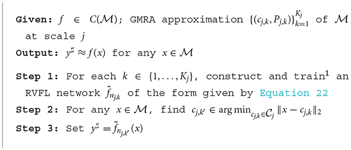
Algorithm 1. Approximation algorithm.

holds with high probability, provided $n_{j,k^{\prime }}$ satisfies the requirements of Theorem 8.

Remark 7 In the RVFL network construction proposed above, we require that the function f be defined in a sufficiently large region around the manifold. Essentially, we need to ensure that f is continuously defined on the set $S:=\mathcal{M}\cup {\hat{\mathcal{M}}}_j$, where ${\hat{\mathcal{M}}}_j$ is the scale-j GMRA approximation

${\hat{\mathcal{M}}}_j:=\left\{P_{j,k_j(z)}z:||z|{|}_2\le \text{rad}(\mathcal{M})\right\}\cap B_2^N(0,\text{rad}(\mathcal{M})).$

This ensures that f can be evaluated on the affine subspaces given by the GMRA.

To simulate Algorithm 1, we take $\mathcal{M}=S^2$ embedded in ℝ²⁰ and construct a GMRA up to level j_max = 15 using 20,000 data points sampled uniformly from $\mathcal{M}$. Given j ≤ j_max, we generate RVFL networks ${\widehat{f}}_{n_{j,k}}:{ℝ}^2\to ℝ$ as in Equation 22 and train them on $V_{j,k}^T(B_2^N(c_{j,k},r)\cap T_{j,k})$ using the training pairs ${\left\{(V_{k,j}^T{x}_{\ell },f(P_{j,k}{x}_{\ell }))\right\}}_{\ell =1}^p$, where T_k,j is the affine space generated by (c_j,k, P_j,k). For simplicity, we fix n_j,k = n to be constant for all k ∈ {1, …, K_j} and use a single, fixed pair of parameters α, Ω > 0 when constructing all RVFL networks. We then randomly select a test set of 200 points $x\in \mathcal{M}$ for use throughout all experiments. In each experiment (i.e., point in Figure 1), we use Algorithm 1 to produce an approximation $y^{♯}={\tilde{f}}_{n_{j,k^{\prime }}}(x)$ of f(x). Figure 1 displays the mean relative error in these approximations for varying numbers of nodes n; to construct this plot, f is taken to be the exponential $f(x)=exp(\sum _{k=1}^{N}x(k))$ and ρ the hyperbolic secant function. Notice that for small numbers of nodes, the RVFL networks are not very good at approximating f, regardless of the choice of α, Ω > 0. However, the error decays as the number of nodes increases until reaching a floor due to error inherent in the GMRA approximation. Hence, as suggested by Theorem 3, to achieve a desired error bound of ε > 0, one needs to only choose a GMRA scale j such that the inherent error in the GMRA (which scales like 2^−j) is less than ε, then adjust the parameters α_j, Ω_j, and n_j,k accordingly.

Figure 1

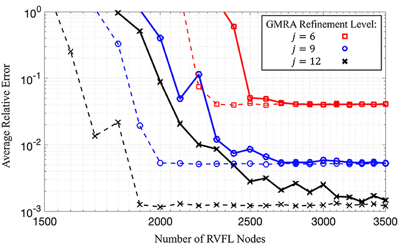
Figure 1. Log-scale plot of average relative error for Algorithm 1 as a function of the number of nodes n in each RVFL network. Black (cross), blue (circle), and red (square) lines correspond to GMRA refinement levels j = 12, j = 9, and j = 6 (resp.). For each j, we fix α_j = 2 and vary Ω_j = 10, 15 (solid and dashed lines, resp.). Reconstruction error decays as a function of n until reaching a floor due to error in the GMRA approximation of $\mathcal{M}$. The code used to obtain these numerical results is available upon direct request sent to the corresponding author.

Remark 8 As we just mentioned, the error can only decay so far due to the resolution of the GMRA approximation. However, that is not the only floor in our simulation; indeed, the ε in Theorem 3 is determined by the α_j's and Ω_j's, which we kept fixed (see the caption of Figure 1). Consequently, the stagnating accuracy as n increases, as seen in Figure 1, is also predicted by Theorem 3. Since the solid and dashed lines seem to reach the same floor, the floor due to error inherent in the GMRA approximation seems to be the limiting error term for RVFL networks with large numbers of nodes.

Remark 9 Utilizing random inner weights and biases resulted in us needing to approximate the atlas to the manifold. To this end, knowing the computational complexity of the GMRA approximation would be useful in practice. As it turns out in Liao and Maggioni [45], calculating the GMRA approximation has computational complexity O(C^dNmlog(m)), where m is the number of training data points and C > 0 is a numerical constant.

3.5 Proofs of technical lemmas

3.5.1 Proof of Lemma 3

Observe that h_Ω defined in Equation 3 may be viewed as a multidimensional bump function; indeed, the parameter Ω > 0 controls the width of the bump. In particular, if Ω is allowed to grow very large, then h_Ω becomes very localized near the origin. Objects that behave in this way are known in the functional analysis literature as approximate δ-functions:

Definition 2 A sequence of functions ${\left\{{\phi }_t\right\}}_{t>0}\subset L^1({ℝ}^N)$ are called approximate (or nascent) δ-functions if

${\displaystyle \underset{t\to \infty }{lim}}{\displaystyle {\int }_{{ℝ}^N}}{\phi }_t(x)f(x)\text{d}x=f(0)$

for all $f\in C_c({ℝ}^N)$. For such functions, we write ${\delta }_0(x)=\underset{t\to \infty }{lim}{\phi }_t(x)$ for all x ∈ ℝ^N, where δ₀ denotes the N-dimensional Dirac δ-function centered at the origin.

Given φ ∈ L¹(ℝ^N) with ${\int }_{{ℝ}^N}\phi (x)\text{d}x=1$, one may construct approximate δ-functions for t > 0 by defining ${\phi }_t(x):=t^N\phi (tx)$ for all x ∈ ℝ^N [46]. Such sequences of approximate δ-functions are also called approximate identity sequences [47] since they satisfy a particularly nice identity with respect to convolution, namely, $\underset{t\to \infty }{lim}\parallel f*{\phi }_t-f{\parallel }_1=0$ for all $f\in C_c({ℝ}^N)$ [see 47, Theorem 6.32]. In fact, such an identity holds much more generally.

Lemma 6 [46, Theorem 1.18] Let φ ∈ L¹(ℝ^N) with ${\int }_{{ℝ}^N}\phi (x)\text{d}x=1$ and for t > 0 define ${\phi }_t(x):=t^N\phi (tx)$ for all x ∈ ℝ^N. If f ∈ L^p(ℝ^N) for 1 ≤ p < ∞ (or $f\in C_0({ℝ}^N)\subset L^{\infty }({ℝ}^N)$ for p = ∞), then $\underset{t\to \infty }{lim}\parallel f*{\phi }_t-f{\parallel }_p=0$.

To prove Equation 4, it would suffice to have $\underset{\Omega \to \infty }{lim}\parallel f*h_{\Omega }-f{\parallel }_{\infty }=0,$ which is really just Lemma 6 in case p = ∞. Nonetheless, we present a proof by mimicking [46] for completeness. Moreover, we will use a part of proof in Remark 10 below.

Lemma 7 Let h ∈ L¹(ℝⁿ) with ${\int }_{{ℝ}^N}h(x)\text{d}x=1$ and define $h_{\Omega }\in L^1({ℝ}^N)$ as in Equation 3 for all Ω > 0. Then, for all $f\in C_0({ℝ}^N)$, we have

${\displaystyle \underset{\Omega \to \infty }{lim}}{\displaystyle \underset{x\in {ℝ}^N}{sup}}|(f*h_{\Omega })(x)-f(x)|=0.$

Proof. By symmetry of the convolution operator in its arguments, we have

$\begin{array}{l}\underset{x\in {ℝ}^N}{\sup }\text{|}(f*h_{\Omega })(x)-f(x)|=\underset{x\in {ℝ}^N}{\sup }\text{|}{\displaystyle {\int }_{{ℝ}^N}f}(y)h_{\Omega }(x-y)\text{d}y-f(x)|\\ =\underset{x\in {ℝ}^N}{\sup }\text{|}{\displaystyle {\int }_{{ℝ}^N}f}(x-y)h_{\Omega }(y)\text{d}y-f(x)|.\end{array}$

Since a simple substitution yields $1={\displaystyle {\int }_{{ℝ}^N}h}(x)\text{d}x={\displaystyle {\int }_{{ℝ}^N}{h}_{\Omega }}(x)\text{d}x,$ it follows that

$\begin{array}{r}{\displaystyle \underset{x\in {ℝ}^N}{sup}}|(f*h_{\Omega })(x)-f(x)|={\displaystyle \underset{x\in {ℝ}^N}{sup}}|{\displaystyle {\int }_{{ℝ}^N}}|f(x-y)-f(x)|h_{\Omega }(y)\text{d}y|\\ \le {\displaystyle {\int }_{{ℝ}^N}}|h_{\Omega }(y)|{\displaystyle \underset{x\in {ℝ}^N}{sup}}|f(x)-f(x-y)|\text{d}y.\end{array}$

Finally, expanding the function h_Ω, we obtain

$\begin{array}{l}{\displaystyle \underset{x\in {ℝ}^N}{sup}}|(f*h_{\Omega })(x)-f(x)|\\ \le {\displaystyle {\int }_{{ℝ}^N}}({\Omega }^N|h(\Omega y)|){\displaystyle \underset{x\in {ℝ}^N}{sup}}|f(x)-f(x-y)|\text{d}y\\ ={\displaystyle {\int }_{{ℝ}^N}}|h(z)|{\displaystyle \underset{x\in {ℝ}^N}{sup}}|f(x)-f(x-z/\Omega )|\text{d}z,\end{array}$

where we have used the substitution z = Ωy. Taking limits on both sides of this expression and observing that

${\displaystyle {\int }_{{ℝ}^N}}|h(z)|{\displaystyle \underset{x\in {ℝ}^N}{sup}}|f(x)-f(x-z/\Omega )|\text{d}z\le 2\parallel h{\parallel }_1{\displaystyle \underset{x\in {ℝ}^N}{sup}}|f(x)|<\infty ,$

using the Dominated Convergence Theorem, we obtain

$\begin{array}{l}{\displaystyle \underset{\Omega \to \infty }{lim}}{\displaystyle \underset{x\in {ℝ}^N}{sup}}|(f*h_{\Omega })(x)-f(x)|\\ \le {\displaystyle {\int }_{{ℝ}^N}}|h(z)|{\displaystyle {lim}_{\Omega \to \infty }}{\displaystyle {sup}_{x\in {ℝ}^N}}|f(x)-f(x-z/\Omega )|\text{d}z.\end{array}$

So, it suffices to show that, for all z ∈ ℝ^N,

${\displaystyle \underset{\Omega \to \infty }{lim}}{\displaystyle \underset{x\in {ℝ}^N}{sup}}|f(x)-f(x-z/\Omega )|=0.$

To this end, let ε > 0 and z ∈ ℝ^N be arbitrary. Since $f\in C_0({ℝ}^N)$, there exists r > 0 sufficiently large such that |f(x)| < ε/2 for all $x\in {ℝ}^N\backslash \overline{B(0,r)}$, where $\overline{B(0,r)}\subset {ℝ}^N$ is the closed ball of radius r centered at the origin. Let $\mathcal{B}:=\overline{B(0,r+\parallel z/\Omega {\parallel }_2)},$ so that for each $x\in {ℝ}^N\backslash \mathcal{B}$ we have both x and x−z/Ω in ${ℝ}^N\backslash \overline{B(0,r)}$. Thus, both |f(x)| < ε/2 and |f(x−z/Ω)| < ε/2, implying that

${\displaystyle \underset{x\in {ℝ}^N\backslash B}{sup}}|f(x)-f(x-z/\Omega )|<\epsilon .$

Hence, we obtain

$\begin{array}{l}{\displaystyle \underset{\Omega \to \infty }{lim}}{\displaystyle \underset{x\in {ℝ}^N}{sup}}|f(x)-f(x-z/\Omega )|\\ \le {\displaystyle \underset{\Omega \to \infty }{lim}}max\{{\displaystyle \underset{x\in B}{sup}}|f(x)-f(x-z/\Omega )|,\\ {\displaystyle \underset{x\in {ℝ}^N\backslash B}{sup}}|f(x)-f(x-z/\Omega )|\}\\ \le max\{\epsilon ,{\displaystyle \underset{\Omega \to \infty }{lim}}{\displaystyle \underset{x\in B}{sup}}|f(x)-f(x-z/\Omega )|\}.\end{array}$

Now, as $\mathcal{B}$ is a compact subset of ℝ^N, the continuous function f is uniformly continuous on $\mathcal{B}$, and so the remaining limit and supremum may be freely interchanged, whereby continuity of f yields

${\displaystyle \underset{\Omega \to \infty }{lim}}{\displaystyle \underset{x\in B}{sup}}|f(x)-f(x-z/\Omega )|={\displaystyle \underset{x\in B}{sup}}{\displaystyle \underset{\Omega \to \infty }{lim}}|f(x)-f(x-z/\Omega )|=0.$

Since ε > 0 may be taken arbitrarily small, we have proved the result.

Remark 10 While Lemma 7 does the approximation we aim for, it gives no indication of how fast

${\displaystyle \underset{x\in {ℝ}^N}{sup}}|(f*h_{\Omega })(x)-f(x)|$

decays in terms of Ω or the dimension N. Assuming h(z) = g(z(1))⋯g(z(N)) for some non-negative g (which is how we will choose h in Section 3.5.2) and f to be β-Hölder continuous for some fixed β ∈ (0, 1) yields that

$\begin{array}{l}{\displaystyle \underset{x\in {ℝ}^N}{sup}}|(f*h_{\Omega })(x)-f(x)|\\ \le {\displaystyle {\int }_{{ℝ}^N}}|h(z)|{\displaystyle \underset{x\in {ℝ}^N}{sup}}|f(x)-f(x-z/\Omega )|\text{d}z\\ \lesssim {\Omega }^{-\beta }{\displaystyle {\int }_{{ℝ}^N}}\parallel z{\parallel }_2^{\beta }h(z)\text{d}z\\ \le {\Omega }^{-\beta }({\displaystyle {\int }_{{ℝ}^N}}(z{(1)}^2+\cdots +z{(N)}^2)h(z)\text{d}z{)}^{\beta /2}\\ \le {\Omega }^{-\beta }(N{\displaystyle \underset{j\in \left\{1,\dots ,N\right\}}{max}}{\displaystyle {\int }_{{ℝ}^N}}z{(j)}^{2}h(z)\text{d}z{)}^{\beta /2}\\ ={(\sqrt{N}/\Omega )}^{\beta }({\displaystyle \underset{j\in \left\{1,\dots ,N\right\}}{max}}{\displaystyle {\int }_{ℝ}}z{(j)}^{2}g(z(j))\text{d}z(j){)}^{\beta /2}\\ ={(\sqrt{N}/\Omega )}^{\beta }({\displaystyle {\int }_{ℝ}}z{(1)}^{2}g(z(1))\text{d}z(1){)}^{\beta /2}\\ \lesssim {(\sqrt{N}/\Omega )}^{\beta }\end{array}$

where the third inequality follows from Jensen's inequality.

3.5.2 Proof of Lemma 4: the limit-integral representation

Let A ∈ C^∞(ℝ) be any even function supported on $\left[-\frac{1}{2},\frac{1}{2}\right]$ s.t. ∥A∥₂ = 1. Then, ϕ = A*A ∈ C^∞(ℝ) is an even function supported on [−1, 1] s.t. ϕ(0) = 1. Lemma 3 implies that

$\begin{array}{ll}f(x)={\displaystyle \underset{\Omega \to \infty }{lim}}(f*h_{\Omega })(x)& (23)\end{array}$

uniformly in x ∈ K for any h ∈ L¹(ℝ^N) satisfying ${\int }_{{ℝ}^N}h(z)\text{d}z=1.$ We choose

$h(z)=\frac{1}{{(2\pi )}^N}{\displaystyle {\int }_{{ℝ}^N}}exp(i\langle w,z\rangle ){\displaystyle \prod _{j=1}^N}\varphi (w(j))\text{d}w$

which the reader may recognize as the (inverse) Fourier transform of ${\prod }_{j=1}^N\varphi (w(j))$. As we announced in Remark 10, h(z) = g(z(1))⋯g(z(N)), where (using the convolution theorem)

$\begin{array}{l}g(z(j))=\frac{1}{2\pi }{\displaystyle {\int }_{ℝ}}exp(iw(j)z(j))\varphi (w(j))\text{d}w(j)\\ =\frac{1}{2\pi }{\displaystyle {\int }_{ℝ}}exp(iw(j)z(j))(A*A)(w(j))\text{d}w(j)\\ =2\pi (\frac{1}{2\pi }{\displaystyle {\int }_{ℝ}}exp(iw(j)z(j))A(w(j))\text{d}w(j){)}^2\ge 0\end{array}$

Moreover, since g is the Fourier transform of an even function, h is real-valued and also even. In addition, since ϕ is smooth, h decays faster than the reciprocal of any polynomial (as follows from repeated integration by parts and the Riemann–Lebesgue lemma), so h ∈ L¹(ℝ^N). Thus, Fourier inversion yields

${\displaystyle {\int }_{{ℝ}^N}}h(z)\text{d}z={\displaystyle {\int }_{{ℝ}^N}}exp(-i\langle w,z\rangle )h(z)\text{d}z{|}_{w=0}={\displaystyle \prod _{j=1}^N}\varphi (0)=1,$

which justifies our application of Lemma 3. Expanding the right-hand side of Equation 23 (using the scaling property of the Fourier transform) yields that

$\begin{array}{l}(f*h_{\Omega })(x)={\displaystyle {\int }_{{ℝ}^N}}f(y)h_{\Omega }(x-y)\text{d}y\\ =\frac{1}{{(2\pi )}^N}{\displaystyle {\int }_K}f(y){\displaystyle {\int }_{{ℝ}^N}}exp(i\langle w,x-y\rangle )\\ {\displaystyle \prod _{j=1}^N}\varphi (w(j)/\Omega )\text{d}w\text{d}y\\ =\frac{1}{{(2\pi )}^N}{\displaystyle {\int }_K}{\displaystyle {\int }_{{\left[-\Omega ,\Omega \right]}^N}}f(y)cos(\langle w,x-y\rangle )\\ {\displaystyle \prod _{j=1}^N}\varphi (w(j)/\Omega )\text{d}w\text{d}y& (24)\end{array}$

because ϕ is even and supported on [−1, 1]. Since Equation 24 is an iterated integral of a continuous function over a compact set, Fubini's theorem readily applies, yielding

$\begin{array}{l}f(x)={\displaystyle \underset{\Omega \to \infty }{lim}}(f*h_{\Omega })(x)\\ ={\displaystyle \underset{\Omega \to \infty }{lim}}\frac{1}{{(2\pi )}^N}{\displaystyle {\int }_{K\times {\left[-\Omega ,\Omega \right]}^N}}f(y)cos(\langle w,x-y\rangle ){\displaystyle \prod _{j=1}^N}\varphi (w(j)/\Omega )\text{d}y\text{d}w.\end{array}$

Since $|\langle w,x-y\rangle |\le \parallel x-y{\parallel }_1\parallel w{\parallel }_{\infty }\le 2N\text{rad}(K)\Omega \le (L+\frac{1}{2})\pi ,$ it follows that

$\begin{array}{r}f(x)={\displaystyle \underset{\Omega \to \infty }{lim}}\frac{1}{{(2\pi )}^N}{\displaystyle {\int }_{K\times {\left[-\Omega ,\Omega \right]}^N}}f(y){cos}_{\Omega }(\langle w,x-y\rangle )\\ {\displaystyle \prod _{j=1}^N}\varphi (w(j)/\Omega )\text{d}y\text{d}w& (25)\end{array}$

where cos_Ω is defined in Equation 5.

With the representation given by Equation 25 in hand, we now seek to reintroduce the general activation function ρ. To this end, since cos_Ω ∈ C_c(ℝ)⊂C₀(ℝ) we may apply the convolution identity given by Equation 4 with f replaced by cos_Ω to obtain ${cos}_{\Omega }(z)=\underset{\alpha \to \infty }{lim}({cos}_{\Omega }*h_{\alpha })(z)$ uniformly for all z ∈ ℝ, where h_α(z) = αρ(αz). Using this representation of cos_Ω in Equation 25, it follows that

$\begin{array}{r}f(x)={\displaystyle \underset{\Omega \to \infty }{lim}}\frac{1}{{(2\pi )}^N}{\displaystyle {\int }_{K\times {\left[-\Omega ,\Omega \right]}^N}}f(y)({\displaystyle \underset{\alpha \to \infty }{lim}}({cos}_{\Omega }*h_{\alpha })(\langle w,x-y\rangle ))\\ {\displaystyle \prod _{j=1}^N}\varphi (w(j)/\Omega )\text{d}y\text{d}w\end{array}$

holds uniformly for all x ∈ K. Since f is continuous and the convolution cos_Ω*h_α is uniformly continuous and uniformly bounded in α by ∥ρ∥₁ (see below), the fact that the domain K×[−Ω, Ω]^N is compact then allows us to bring the limit as α tends to infinity outside the integral in this expression via the Dominated Convergence Theorem, which gives us

$\begin{array}{r}f(x)={\displaystyle \underset{\Omega \to \infty }{lim}}{\displaystyle \underset{\alpha \to \infty }{lim}}\frac{1}{{(2\pi )}^N}{\displaystyle {\int }_{K\times {\left[-\Omega ,\Omega \right]}^N}}f(y)({cos}_{\Omega }*h_{\alpha })\\ (\langle w,x-y\rangle ){\displaystyle \prod _{j=1}^N}\varphi (w(j)/\Omega )\text{d}y\text{d}w& (26)\end{array}$

uniformly for every x ∈ K. The uniform boundedness of the convolution follows from the fact that

$\begin{array}{l}({cos}_{\Omega }*h_{\alpha })(z)={\displaystyle {\int }_{ℝ}}{cos}_{\Omega }(z-u)h_{\alpha }(u)\text{d}u\\ ={\displaystyle {\int }_{ℝ}}{cos}_{\Omega }(z-v/\alpha )\rho (v)\text{d}v,& (27)\end{array}$

where v = αu.

Remark 11 It should be noted that we are unable to swap the order of the limits in Equation 26, since cos_Ω is not in C₀(ℝ) when Ω is allowed to be infinite.

Remark 12 Complementing Remark 10, we will now elucidate how fast

$\begin{array}{l}|{cos}_{\Omega }(z)-({cos}_{\Omega }*h_{\alpha })(z)|\end{array}$

decays in terms of α. Using the fact that ${\int }_{ℝ}\rho (z)\text{d}z=1,$ Equation 27 and the triangle inequality allows us to bound the absolute difference above by

$\begin{array}{l}{\displaystyle {\int }_{ℝ}}|{cos}_{\Omega }(z)-{cos}_{\Omega }(z-v/\alpha )|·|\rho (v)|\text{d}v.\end{array}$

Since cos_Ω is 1-Lipschitz, it follows that the above integral is bounded by ${\int }_{ℝ}|v\rho (v)|dv/\alpha .$

To complete this step of the proof, observe that the definition of cos_Ω allows us to write

$\begin{array}{l}({cos}_{\Omega }*h_{\alpha })(z)=\alpha {\displaystyle {\int }_{ℝ}}{cos}_{\Omega }(u)\rho |\alpha (z-u)|\text{d}u\\ =\alpha {\displaystyle {\int }_{-\frac{\pi }{2}(2L+1)}^{\frac{\pi }{2}(2L+1)}}{cos}_{\Omega }(u)\rho (\alpha (z-u))\text{d}u& (28)\end{array}$

By substituting Equation 28 into Equation 26, we then obtain

$\begin{array}{r}f(x)={\displaystyle \underset{\Omega \to \infty }{lim}}{\displaystyle \underset{\alpha \to \infty }{lim}}\frac{\alpha }{{(2\pi )}^N}{\displaystyle {\int }_{K(\Omega )}}f(y){cos}_{\Omega }(u)\rho (\alpha (\langle w,x-y\rangle -u))\\ {\displaystyle \prod _{j=1}^N}\varphi (w(j)/\Omega )\text{d}y\text{d}w\text{d}u\end{array}$

uniformly for all x ∈ K, where $K(\Omega ):=K\times {\left[-\Omega ,\Omega \right]}^N\times \left[-\frac{\pi }{2}(2L+1),\frac{\pi }{2}(2L+1)\right]$. In this way, recalling that $F_{\alpha ,\Omega }(y,w,u):=\frac{\alpha }{{(2\pi )}^N}f(y){cos}_{\Omega }(u){\prod }_{j=1}^N\varphi (w(j)/\Omega ),$ and b_α(y, w, u): = −α(〈w, y〉+u) for y, w ∈ ℝ^N and u ∈ ℝ, we conclude the proof.

3.5.3 Proof of Lemma 5: Monte-Carlo integral approximation

The next step in the proof of Theorem 5 is to approximate the integral in Equation 7 using the Monte-Carlo method. To this end, let ${\left\{y_k\right\}}_{k=1}^n$, ${\left\{w_k\right\}}_{k=1}^n$, and ${\left\{u_k\right\}}_{k=1}^n$ be independent samples drawn uniformly from K, [−Ω, Ω]^N, and $\left[-\frac{\pi }{2}(2L+1),\frac{\pi }{2}(2L+1)\right]$, respectively, and consider the sequence of random variables ${\left\{I_n(x)\right\}}_{n=1}^{\infty }$ defined by

$\begin{array}{ll}{I}_n(x):=\frac{\text{vol}(K(\Omega ))}{n}{\displaystyle \sum _{k=1}^n}{F}_{\alpha ,\Omega }(y_k,w_k,u_k)\rho (\alpha \langle w_k,x\rangle +b_{\alpha }(y_k,w_k,u_k))& (29)\end{array}$

for each x ∈ K, where we note that vol(K(Ω)) = (2Ω)^Nπ(2L + 1)vol(K). If we also define

$\begin{array}{l}I(x;p):={\displaystyle {\int }_{K(\Omega )}}(F_{\alpha ,\Omega }(y,w,u)\rho (\alpha \langle w,x\rangle +b_{\alpha }(y,w,u)){)}^p\text{d}y\text{d}w\text{d}u\end{array}$

for x ∈ K and p ∈ ℕ, then we want to show that

$\begin{array}{ll}𝔼{\displaystyle {\int }_K}|I(x;1)-I_n(x){|}^2\text{d}x=O(1/n)& (30)\end{array}$

as n → ∞, where the expectation is taken with respect to the joint distribution of the random samples ${\left\{y_k\right\}}_{k=1}^n$, ${\left\{w_k\right\}}_{k=1}^n$, and ${\left\{u_k\right\}}_{k=1}^n$. For this, it suffices to find a constant C(f, ρ, α, Ω, N) < ∞ independent of n satisfying

${\displaystyle {\int }_K}𝔼|I(x;1)-I_n(x){|}^2\text{d}x\le \frac{C(f,\rho ,\alpha ,\Omega ,N)}{n}.$

Indeed, an application of Fubini's theorem would then yield

$𝔼{\displaystyle {\int }_K}|I(x;1)-I_n(x){|}^2\text{d}x\le \frac{C(f,\rho ,\alpha ,\Omega ,N)}{n},$

which implies Equation 30. To determine such a constant, we first observe by Theorem 4 that

$𝔼|I(x;1)-I_n(x){|}^2=\frac{\text{vo}{\text{l}}^2(K(\Omega ))\sigma {(x)}^2}{n},$

where we define the variance term

$\sigma {(x)}^2:=\frac{I(x;2)}{\text{vol}(K(\Omega ))}-\frac{I{(x;1)}^2}{\text{vo}{\text{l}}^2(K(\Omega ))}$

for x ∈ K. Since ∥ϕ∥_∞ = 1 (see Lemma 8 below), it follows that

$|F_{\alpha ,\Omega }(y,w,u)|=\frac{\alpha }{{(2\pi )}^N}|f(y)|·|{cos}_{\Omega }(u)|{\displaystyle \prod _{j=1}^N}|\varphi (w(j)/\Omega )|\le \frac{\alpha M}{{(2\pi )}^N}$

for all y, w ∈ ℝ^N and u ∈ ℝ, where $M:=\underset{x\in K}{sup}|f(x)|<\infty$, we obtain the following simple bound on the variance term

$\begin{array}{l}\sigma {(x)}^2\le \frac{I(x;2)}{\text{vol}(K(\Omega ))}\le \frac{{\alpha }^2{M}^2}{{(2\pi )}^{2N}\text{vol}(K(\Omega ))}\\ {\displaystyle {\int }_{K(\Omega )}}|\rho (\alpha \langle w,x\rangle +b_{\alpha }(y,w,u)){|}^2\text{d}y\text{d}w\text{d}u.\end{array}$

Since we assume ρ ∈ L^∞(ℝ), we then have

$\begin{array}{c}{\displaystyle {\int }_K}𝔼|I(x;1)-I_n(x){|}^2\text{d}x=\frac{\text{vo}{\text{l}}^2(K(\Omega ))}{n}{\displaystyle {\int }_K}\sigma {(x)}^2\text{d}x\\ \le \frac{{\alpha }^2{M}^2\text{vol}(K(\Omega ))}{{(2\pi )}^{2N}n}{\displaystyle {\int }_{K\times K(\Omega )}}|\rho (\alpha \langle w,x\rangle +b_{\alpha }(y,w,u)){|}^2\text{d}x\text{d}y\text{d}w\text{d}u\\ =\frac{{\alpha }^2{M}^2\text{vo}{\text{l}}^2(K(\Omega ))\text{vol}(K)\Vert \rho {\Vert }_{\infty }^2}{{(2\pi )}^{2N}n}.\end{array}$

Substituting the value of vol(K(Ω)), we obtain

$C(f,\rho ,\alpha ,\Omega ,N):={\alpha }^2{M}^2{(\Omega /\pi )}^{2N}{\pi }^2{(2L+1)}^2\text{vo}{\text{l}}^3(K)\Vert \rho {\Vert }_{\infty }^2$

is a suitable choice for the desired constant.

Now that we have established Equation 30, we may rewrite the random variables I_n(x) in a more convenient form. To this end, we change the domain of the random samples ${\left\{w_k\right\}}_{k=1}^n$ to [−αΩ, αΩ]^N and define the new random variables ${\left\{b_k\right\}}_{k=1}^n\subset ℝ$ by b_k: = −(〈w_k, y_k〉+αu_k) for each k = 1, …, n. In this way, if we denote

$v_k:=\frac{\text{vol}(K(\Omega ))}{n}{F}_{\alpha ,\Omega }(y_k,\frac{w_k}{\alpha },u_k)$

for each k = 1, …, n, the random variables ${\left\{f_n\right\}}_{n=1}^{\infty }$ defined by

$f_n(x):={\displaystyle \sum _{k=1}^n}{v}_k\rho (\langle w_k,x\rangle +b_k)$

satisfy f_n(x) = I_n(x) for every x ∈ K. Combining this with Equation 30, we have proved Lemma 5.

Lemma 8 ∥ϕ∥_∞ = 1.

Proof. It suffices to prove that |ϕ(z)| ≤ 1 for all z ∈ ℝ because ϕ(0) = 1. By Cauchy–Schwarz,

$\begin{array}{l}|\varphi (z)|=|{\displaystyle {\int }_{ℝ}}A(u)A(z-u)\text{d}u|\\ \le \sqrt{{\displaystyle {\int }_{ℝ}}A(u)A(u)\text{d}u{\displaystyle {\int }_{ℝ}}A(z-u)A(z-u)\text{d}u}\\ =\sqrt{{\displaystyle {\int }_{ℝ}}A(u)A(0-u)\text{d}u{\displaystyle {\int }_{ℝ}}A(v)A(-v)\text{d}v}=\sqrt{\varphi (0)\varphi (0)}=1\end{array}$

because A is even.

3.5.4 Proof of Theorem 1 when ρ′ ∈ L¹(ℝ)∩L^∞(ℝ)

Let $f\in C_c({ℝ}^N)$ with K: = supp(f) and suppose ε > 0 is fixed. Take the activation function ρ:ℝ → ℝ to be differentiable with ρ′ ∈ L¹(ℝ)∩L^∞(ℝ). We wish to show that there exists a sequence of RVFL networks ${\left\{f_n\right\}}_{n=1}^{\infty }$ defined on K which satisfy the asymptotic error bound

$𝔼{\displaystyle {\int }_K}|f(x)-f_n(x){|}^2\text{d}x\le \epsilon +O(1/n)$

as n → ∞. The proof of this result is a minor modification of second step in the proof of Theorem 5.

If we redefine h_α(z) as αρ′(αz), then Equation 26 plainly still holds and Equation 28 reads

$({cos}_{\Omega }*h_{\alpha })(z)=\alpha {\displaystyle {\int }_{ℝ}}{cos}_{\Omega }(u){\rho }^{\prime }(\alpha (z-u))\text{d}u.$

Recalling the definition of cos_Ω in Equation 5 and integrating by parts, we obtain

$\begin{array}{l}({cos}_{\Omega }*h_{\alpha })(z)=\alpha {\displaystyle {\int }_{ℝ}}{cos}_{\Omega }(u){\rho }^{\prime }(\alpha (z-u))\text{d}u\\ =-{\displaystyle {\int }_{-\frac{\pi }{2}(2L+1)}^{\frac{\pi }{2}(2L+1)}}{cos}_{\Omega }(u)d\rho (\alpha (z-u))\\ =-{cos}_{\Omega }(u)\rho (\alpha (z-u)){|}_{-\frac{\pi }{2}(2L+1)}^{\frac{\pi }{2}(2L+1)}\\ +{\displaystyle {\int }_{-\frac{\pi }{2}(2L+1)}^{\frac{\pi }{2}(2L+1)}}\rho (\alpha (z-u))d{cos}_{\Omega }(u)\\ =-{\displaystyle {\int }_{ℝ}}{sin}_{\Omega }(u)\rho (\alpha (z-u))\text{d}u\end{array}$

for all z ∈ ℝ, where $L:=\lceil \frac{2N}{\pi }\text{rad}(K)\Omega -\frac{1}{2}\rceil$ and sin_Ω:ℝ → [−1, 1] is defined analogously to Equation 5. Substituting this representation of (cos_Ω*h_α)(z) into Equation 26 then yields

$\begin{array}{l}f(x)={\displaystyle \underset{\Omega \to \infty }{lim}}{\displaystyle \underset{\alpha \to \infty }{lim}}\frac{-\alpha }{{(2\pi )}^N}{\displaystyle {\int }_{K(\Omega )}}f(y){sin}_{\Omega }(u)\rho (\alpha (\langle w,x-y\rangle -u))\\ {\displaystyle \prod _{j=1}^N}\varphi (w(j)/\Omega )\text{d}y\text{d}w\text{d}u\end{array}$

uniformly for every x ∈ K. Thus, if we replace the definition of F_{α, Ω} in Equation 6 by

$F_{\alpha ,\Omega }(y,w,u):=\frac{-\alpha }{{(2\pi )}^N}f(y){sin}_{\Omega }(u){\displaystyle \prod _{j=1}^N}\varphi (w(j)/\Omega )$

for y, w ∈ ℝ^N and u ∈ ℝ, we again obtain the uniform representation given by Equation 7 for all x ∈ K. The remainder of the proof proceeds from this point exactly as in the proof of Theorem 5.

3.5.5 Proof of Theorem 8

We wish to show that there exist sequences of RVFL networks ${\left\{{\tilde{f}}_{n_j}\right\}}_{n_j=1}^{\infty }$ defined on ϕ_j(U_j) for each j ∈ J, which together satisfy the error bound

${\displaystyle {\int }_M}|f(x)-{\displaystyle \sum _{\left\{j\in J:x\in U_j\right\}}}({\tilde{f}}_{n_j}\circ {\varphi }_j)(x){|}^2\text{d}x<\epsilon$

with probability at least 1−η for {_{nj}j ∈ J} sufficiently large. The proof is obtained by showing that

$\begin{array}{ll}|f(x)-{\displaystyle \sum _{\left\{j\in J:x\in U_j\right\}}}({\tilde{f}}_{n_j}\circ {\varphi }_j)(x)|<\sqrt{\frac{\epsilon }{\text{vol}(M)}}& (31)\end{array}$

holds uniformly for $x\in \mathcal{M}$ with high probability.

We begin as in the proof of Theorem 7 by applying the representation given by Equation 17 for (f on each chart (U_j, ϕ_j), which gives us

$\begin{array}{l}|f(x)-{\displaystyle \sum _{\left\{j\in J:x\in U_j\right\}}}({\tilde{f}}_{n_j}\circ {\varphi }_j)(x)|\\ \le {\displaystyle \sum _{\left\{j\in J:x\in U_j\right\}}}|({\widehat{f}}_j\circ {\varphi }_j)(x)-({\tilde{f}}_{n_j}\circ {\varphi }_j)(x)|& (32)\end{array}$

for all $x\in \mathcal{M}$. Now, since we have already seen that ${\widehat{f}}_j\in C_c({ℝ}^d)$ for each j ∈ J, Theorem 6 implies that for any ε_j > 0, there exist constants α_j, Ω_j > 0 and hidden-to-output layer weights ${\left\{v_k^{(j)}\right\}}_{k=1}^{n_j}\subset ℝ$ for each j ∈ J such that for any

$\begin{array}{ll}{\delta }_j<\frac{\sqrt{{\epsilon }_j}}{8\sqrt{2d}\kappa {\alpha }_j^2{M}_j{\Omega }_j{({\Omega }_j/\pi )}^d\text{vo}{\text{l}}^{3/2}({\varphi }_j(U_j))(\pi +2d\text{rad}({\varphi }_j(U_j))\Omega )}& (33)\end{array}$

we have

$|{\widehat{f}}_j(z)-{\tilde{f}}_{n_j}(z)|<\sqrt{\frac{{\epsilon }_j}{2\text{vol}({\varphi }_j(U_j))}}$

uniformly for all z ∈ ϕ_j(U_j) with probability at least 1−η_j, provided the number of nodes n_j satisfies

$\begin{array}{lll}{n}_j& \ge \frac{c{\Sigma }^{(j)}{\alpha }_j{({\Omega }_j/\pi )}^d(\pi +2d\text{rad}({\varphi }_j(U_j)){\Omega }_j)log(3{\eta }_j^{-1}N({\delta }_j,{\varphi }_j(U_j)))}{\sqrt{{\epsilon }_j}log(1+\frac{\sqrt{{\epsilon }_j}}{{\Sigma }^{(j)}{\alpha }_j{({\Omega }_j/\pi )}^d(\pi +2d\text{rad}({\varphi }_j(U_j)){\Omega }_j)})},& (34)\end{array}$

where c > 0 is a numerical constant and ${\Sigma }^{(j)}:=2C^{(j)}\sqrt{2\text{vol}({\varphi }_j(U_j))}.$ Indeed, it suffices to choose

$v_k^{(j)}:=\frac{\text{vol}(K({\Omega }_j))}{n_j}{F}_{{\alpha }_j,{\Omega }_j}(y_k^{(j)},\frac{w_k^{(j)}}{{\alpha }_j},u_k^{(j)})$

for each k = 1, …, n_j, where

$K({\Omega }_j):={\varphi }_j(U_j)\times {\left[-{\alpha }_j{\Omega }_j,{\alpha }_j{\Omega }_j\right]}^d\times \left[-\frac{\pi }{2}(2L_j+1),\frac{\pi }{2}(2L_j+1)\right]$

for each j ∈ J. Combined with Equation 32, choosing δ_j and n_j satisfying Equations 33, 34, respectively, then yields

$\begin{array}{l}|f(x)-{\displaystyle \sum _{\left\{j\in J:x\in U_j\right\}}}({\tilde{f}}_{n_j}\circ {\varphi }_j)(x)|<{\displaystyle \sum _{\left\{j\in J:x\in U_j\right\}}}\sqrt{\frac{{\epsilon }_j}{2\text{vol}({\varphi }_j(U_j))}}\\ \le {\displaystyle \sum _{j\in J}}\sqrt{\frac{{\epsilon }_j}{2\text{vol}({\varphi }_j(U_j))}}\end{array}$

for all $x\in \mathcal{M}$ with probability at least $1-\sum _{\left\{j\in J:x\in U_j\right\}}{\eta }_j\ge 1-\sum _{j\in J}{\eta }_j$. Since we require that Equation 31 holds for all $x\in \mathcal{M}$ with probability at least 1−η, the proof is then completed by choosing {_{εj}j ∈ J} and {_{ηj}j ∈ J}, such that

$\epsilon =\frac{\text{vol}(M)}{2}({\displaystyle \sum _{j\in J}}\sqrt{\frac{{\epsilon }_j}{\text{vol}({\varphi }_j(U_j))}}{)}^2\text{and }\eta ={\displaystyle \sum _{j\in J}}{\eta }_j.$

In particular, it suffices to choose

${\epsilon }_j=\frac{2\text{vol}({\varphi }_j(U_j))\epsilon }{|J{|}^2\text{vol}(M)}$

and η_j = η/|J| for each j ∈ J, so that Equations 33, 34 become

$\begin{array}{ll}{\delta }_j& <\frac{\sqrt{\epsilon }}{8|J|\sqrt{d\text{vol}(M)}\kappa {\alpha }_j^2{M}_j{\Omega }_j{({\Omega }_j/\pi )}^d\text{vol}({\varphi }_j(U_j))(\pi +2d\text{rad}({\varphi }_j(U_j))\Omega )},\\ n_j& \ge \frac{2c|J|\sqrt{\text{vol}(M)}{C}^{(j)}{\alpha }_j{({\Omega }_j/\pi )}^d(\pi +2d\text{rad}({\varphi }_j(U_j)){\Omega }_j)log(3|J|{\eta }^{-1}N({\delta }_j,{\varphi }_j(U_j)))}{\sqrt{\epsilon }log(1+\frac{\sqrt{\epsilon }}{2|J|\sqrt{\text{vol}(M)}{C}^{(j)}{\alpha }_j{({\Omega }_j/\pi )}^d(\pi +2d\text{rad}({\varphi }_j(U_j)){\Omega }_j)})},\end{array}$

as desired.

4 Discussion

The central topic of this study is the study of the approximation properties of a randomized variation of shallow neural networks known as RVFL. In contrast with the classical single-layer neural networks, training of an RVFL involves only learning the output weights, while the input weights and biases of all the nodes are selected at random from an appropriate distribution and stay fixed throughout the training. The main motivation for studying the properties of such networks is as follows:

1. Random weights are often utilized as an initialization for a NN training procedure. Thus, establishing the properties of the RVFL networks is an important first step toward understanding how random weights are transformed during training.

2. Due to their much more computationally efficient training process, the RVFL networks proved to be a valuable alternative to the classical SLFNs. They were successfully used in several modern applications, especially those that require frequent re-training of a neural network [20, 26, 27].

Despite their practical and theoretical importance, results providing rigorous mathematical analysis of the properties of RVFLs are rare. The work of Igelnik and Pao [16] showed that RVFL networks are universal approximators for the class of continuous, compactly supported functions and established the asymptotic convergence rate of the expected approximation error as a function of the number of nodes in the hidden layer. While this result served as a theoretical justification for using RVFL networks in practice, a close examination led us to the conclusion that the proofs in Igelnik and Pao [16] contained several technical errors.

In this study, we offer a revision and a modification of the proof methods from Igelnik and Pao [16] that allow us to prove a corrected, slightly weaker version of the result announced by Igelnik and Pao. We further build upon their work and show a non-asymptotic probabilistic (instead of on average) approximation result, which gives an explicit bound on the number of hidden layer nodes that are required to achieve the desired approximation accuracy with the desired level of certainty (that is, with high enough probability). In addition to that, we extend the obtained result to the case when the function is supported on a compact, low-dimensional sub-manifold of the ambient space.

While our study closes some of the gaps in the study of the approximation properties of RVFL, we believe that it just starts the discussion and opens many directions for further research. We briefly outline some of them here.

In our results, the dependence of the required number n of the nodes in the hidden layer on the dimension N of the domain is superexponential, which is likely an artifact of the proof methods we use. We believe this dependence can be improved to be exponential by using a different, more refined approach to the construction of the limit-integral representation of a function. A related interesting direction for future research is to study how the bound on n changes for more restricted classes of (e.g., smooth) functions.

Another important direction that we did not discuss in this study is learning the output weights and studying the robustness of the RVFL approximation to the noise in the training data. Obtaining provable robustness guarantees for an RVFL training procedure would be a step toward the robustness analysis of neural networks.

Data availability statement

The original contributions presented in the study are included in the article/supplementary material, further inquiries can be directed to the corresponding author.

Author contributions

DN: Writing – original draft, Writing – review & editing. AN: Writing – original draft, Writing – review & editing. RS: Writing – original draft, Writing – review & editing. PS: Writing – original draft, Writing – review & editing. OS: Writing – original draft, Writing – review & editing.

Funding

The author(s) declare financial support was received for the research, authorship, and/or publication of this article. DN was partially supported by NSF DMS 2108479 and NSF DMS 2011140. RS was partially supported by a UCSD senate research award and a Simons fellowship. PS was partially supported by NSF DMS 1909457.

Acknowledgments

The authors thank F. Krahmer, S. Krause-Solberg, and J. Maly for sharing their GMRA code, which they adapted from that provided by M. Maggioni.

Conflict of interest

The authors declare that the research was conducted in the absence of any commercial or financial relationships that could be construed as a potential conflict of interest.

Publisher's note

All claims expressed in this article are solely those of the authors and do not necessarily represent those of their affiliated organizations, or those of the publisher, the editors and the reviewers. Any product that may be evaluated in this article, or claim that may be made by its manufacturer, is not guaranteed or endorsed by the publisher.

Author disclaimer

The views expressed in this article are those of the authors and do not reflect the official policy or position of the U.S. Air Force, Department of Defense, or U.S. Government.

Footnotes

1. ^The construction and training of RVFL networks is left as a “black box” procedure. How to best choose a specific activation function ρ(z) and train each RVFL network given by Equation 22 is outside of the scope of this study. The reader may, for instance, select from the range of methods available for training neural networks.

References

1. Krizhevsky A, Sutskever I, Hinton GE. Imagenet classification with deep convolutional neural networks. In: Advances in Neural Information Processing Systems. (2012). p. 1097–105.

Google Scholar

2. Szegedy C, Liu W, Jia Y, Sermanet P, Reed S, Anguelov D, et al. Going deeper with convolutions. In: Proceedings of the IEEE conference on computer vision and pattern recognition. (2015). p. 1–9. doi: 10.1109/CVPR.2015.7298594

Crossref Full Text | Google Scholar

3. He K, Zhang X, Ren S, Sun J. Deep residual learning for image recognition. In: Proceedings of the IEEE Conference on Computer Vision And Pattern Recognition. (2016). p. 770–778. doi: 10.1109/CVPR.2016.90

Crossref Full Text | Google Scholar

4. Huang G, Liu Z, Van Der Maaten L, Weinberger KQ. Densely connected convolutional networks. In: Proceedings of the IEEE Conference on Computer Vision and Pattern Recognition. (2017). p. 4700–4708. doi: 10.1109/CVPR.2017.243

Crossref Full Text | Google Scholar

5. Yang Y, Zhong Z, Shen T, Lin Z. Convolutional neural networks with alternately updated clique. In: Proceedings of the IEEE Conference on Computer Vision and Pattern Recognition. (2018). p. 2413–2422. doi: 10.1109/CVPR.2018.00256

Crossref Full Text | Google Scholar

6. Barron AR. Universal approximation bounds for superpositions of a sigmoidal function. IEEE Trans Inf Theory. (1993) 39:930–45. doi: 10.1109/18.256500

Crossref Full Text | Google Scholar

7. Candés EJ. Harmonic analysis of neural networks. Appl Comput Harm Analysis. (1999) 6:197–218. doi: 10.1006/acha.1998.0248

Crossref Full Text | Google Scholar

8. Vershynin R. Memory capacity of neural networks with threshold and ReLU activations. arXiv preprint arXiv:200106938. (2020).

Google Scholar

9. Baldi P, Vershynin R. The capacity of feedforward neural networks. Neural Netw. (2019) 116:288–311. doi: 10.1016/j.neunet.2019.04.009

PubMed Abstract | Crossref Full Text | Google Scholar

10. Huang GB, Babri HA. Upper bounds on the number of hidden neurons in feedforward networks with arbitrary bounded nonlinear activation functions. IEEE Trans Neural Netw. (1998) 9:224–9. doi: 10.1109/72.655045

PubMed Abstract | Crossref Full Text | Google Scholar

11. Suganthan PN. Letter: On non-iterative learning algorithms with closed-form solution. Appl Soft Comput. (2018) 70:1078–82. doi: 10.1016/j.asoc.2018.07.013

Crossref Full Text | Google Scholar

12. Olson M, Wyner AJ, Berk R. Modern Neural Networks Generalize on Small Data Sets. In: Proceedings of the 32Nd International Conference on Neural Information Processing Systems. NIPS'18. Curran Associates Inc. (2018). p. 3623–3632.

Google Scholar

13. Schmidt WF, Kraaijveld MA, Duin RPW. Feedforward neural networks with random weights. In: Proceedings 11th IAPR International Conference on Pattern Recognition. Vol. II. Conference B: Pattern Recognition Methodology and Systems. (1992). p. 1–4.

Google Scholar

14. Te Braake HAB, Van Straten G. Random activation weight neural net (RAWN) for fast non-iterative training. Eng Appl Artif Intell. (1995) 8:71–80. doi: 10.1016/0952-1976(94)00056-S

Crossref Full Text | Google Scholar

15. Pao YH, Takefuji Y. Functional-link net computing: theory, system architecture, and functionalities. Computer. (1992) 25:76–9. doi: 10.1109/2.144401

Crossref Full Text | Google Scholar

16. Igelnik B, Pao YH. Stochastic choice of basis functions in adaptive function approximation and the functional-link net. IEEE Trans Neur Netw. (1995) 6:1320–9. doi: 10.1109/72.471375

PubMed Abstract | Crossref Full Text | Google Scholar

17. Huang GB, Zhu QY, Siew CK. Extreme learning machine: theory and applications. Neurocomputing. (2006) 70:489–501. doi: 10.1016/j.neucom.2005.12.126

Crossref Full Text | Google Scholar

18. Pao YH, Park GH, Sobajic DJ. Learning and generalization characteristics of the random vector functional-link net. Neurocomputing. (1994) 6:163–80. doi: 10.1016/0925-2312(94)90053-1

Crossref Full Text | Google Scholar

19. Pao YH, Phillips SM. The functional link net and learning optimal control. Neurocomputing. (1995) 9:149–64. doi: 10.1016/0925-2312(95)00066-F

Crossref Full Text | Google Scholar

20. Chen CP, Wan JZ, A. rapid learning and dynamic stepwise updating algorithm for flat neural networks and the application to time-series prediction. IEEE Trans Syst Man Cybern B. (1999) 29:62–72. doi: 10.1109/3477.740166

PubMed Abstract | Crossref Full Text | Google Scholar

21. Park GH, Pao YH. Unconstrained word-based approach for off-line script recognition using density-based random-vector functional-link net. Neurocomputing. (2000) 31:45–65. doi: 10.1016/S0925-2312(99)00149-6

Crossref Full Text | Google Scholar

22. Zhang L, Suganthan PN. Visual tracking with convolutional random vector functional link network. IEEE Trans Cybern. (2017) 47:3243–53. doi: 10.1109/TCYB.2016.2588526

PubMed Abstract | Crossref Full Text | Google Scholar

23. Zhang L, Suganthan PN. Benchmarking ensemble classifiers with novel co-trained kernel ridge regression and random vector functional link ensembles [research frontier]. IEEE Comput Intell Mag. (2017) 12:61–72. doi: 10.1109/MCI.2017.2742867

Crossref Full Text | Google Scholar

24. Katuwal R, Suganthan PN, Zhang L. An ensemble of decision trees with random vector functional link networks for multi-class classification. Appl Soft Comput. (2018) 70:1146–53. doi: 10.1016/j.asoc.2017.09.020

Crossref Full Text | Google Scholar

25. Vuković N, Petrović M, Miljković Z. A comprehensive experimental evaluation of orthogonal polynomial expanded random vector functional link neural networks for regression. Appl Soft Comput. (2018) 70:1083–1096. doi: 10.1016/j.asoc.2017.10.010

Crossref Full Text | Google Scholar

26. Tang L, Wu Y, Yu L, A. non-iterative decomposition-ensemble learning paradigm using RVFL network for crude oil price forecasting. Appl Soft Comput. (2018) 70:1097–108. doi: 10.1016/j.asoc.2017.02.013

Crossref Full Text | Google Scholar

27. Dash Y, Mishra SK, Sahany S, Panigrahi BK. Indian summer monsoon rainfall prediction: A comparison of iterative and non-iterative approaches. Appl Soft Comput. (2018) 70:1122–34. doi: 10.1016/j.asoc.2017.08.055

Crossref Full Text | Google Scholar

28. Henríquez PA, Ruz G. Twitter sentiment classification based on deep random vector functional link. In: 2018 International Joint Conference on Neural Networks (IJCNN). IEEE (2018). p. 1–6. doi: 10.1109/IJCNN.2018.8489703

Crossref Full Text | Google Scholar

29. Katuwal R, Suganthan PN, Tanveer M. Random vector functional link neural network based ensemble deep learning. arXiv preprint arXiv:190700350. (2019).

PubMed Abstract | Google Scholar

30. Zhang Y, Wu J, Cai Z, Du B, Yu PS. An unsupervised parameter learning model for RVFL neural network. Neural Netw. (2019) 112:85–97. doi: 10.1016/j.neunet.2019.01.007

PubMed Abstract | Crossref Full Text | Google Scholar

31. Hornik K. Approximation capabilities of multilayer feedforward networks. Neural Netw. (1991) 4:251–7. doi: 10.1016/0893-6080(91)90009-T

Crossref Full Text | Google Scholar

32. Leshno M, Lin VY, Pinkus A, Schocken S. Multilayer feedforward networks with a nonpolynomial activation function can approximate any function. Neural Netw. (1993) 6:861–7. doi: 10.1016/S0893-6080(05)80131-5

Crossref Full Text | Google Scholar

33. Li JY, Chow WS, Igelnik B, Pao YH. Comments on “Stochastic choice of basis functions in adaptive function approximation and the functional-link net” [with reply]. IEEE Trans Neur Netw. (1997) 8:452–4. doi: 10.1109/72.557702

Crossref Full Text | Google Scholar

34. Burkhardt DB, San Juan BP, Lock JG, Krishnaswamy S, Chaffer CL. Mapping phenotypic plasticity upon the cancer cell state landscape using manifold learning. Cancer Discov. (2022) 12:1847–59. doi: 10.1158/2159-8290.CD-21-0282

PubMed Abstract | Crossref Full Text | Google Scholar

35. Mitchell-Heggs R, Prado S, Gava GP, Go MA, Schultz SR. Neural manifold analysis of brain circuit dynamics in health and disease. J Comput Neurosci. (2023) 51:1–21. doi: 10.1007/s10827-022-00839-3

PubMed Abstract | Crossref Full Text | Google Scholar

36. Dick J, Kuo FY, Sloan IH. High-dimensional integration: the quasi-Monte Carlo way. Acta Numerica. (2013) 22:133–288. doi: 10.1017/S0962492913000044

Crossref Full Text | Google Scholar

37. Ledoux M. The Concentration of Measure Phenomenon. Providence, RI: American Mathematical Soc. (2001).

Google Scholar

38. Massart P. About the constants in Talagrand's deviation inequalities for empirical processes. Technical Report, Laboratoire de statistiques, Universite Paris Sud. (1998).

Google Scholar

39. Talagrand M. New concentration inequalities in product spaces. Invent Mathem. (1996) 126:505–63. doi: 10.1007/s002220050108

Crossref Full Text | Google Scholar

40. Shaham U, Cloninger A, Coifman RR. Provable approximation properties for deep neural networks. Appl Comput Harmon Anal. (2018) 44:537–57. doi: 10.1016/j.acha.2016.04.003

Crossref Full Text | Google Scholar

41. Tu LW. An Introduction to Manifolds. New York: Springer. (2010). doi: 10.1007/978-1-4419-7400-6_3

Crossref Full Text | Google Scholar

42. Allard WK, Chen G, Maggioni M. Multi-scale geometric methods for data sets II: geometric multi-resolution analysis. Appl Comput Harmon Anal. (2012) 32:435–62. doi: 10.1016/j.acha.2011.08.001

Crossref Full Text | Google Scholar

43. Iwen MA, Krahmer F, Krause-Solberg S, Maly J. On recovery guarantees for one-bit compressed sensing on manifolds. Discr Comput Geom. (2018) 65:953–998. doi: 10.1109/SAMPTA.2017.8024465

Crossref Full Text | Google Scholar

44. Maggioni M, Minsker S, Strawn N. Multiscale dictionary learning: non-asymptotic bounds and robustness. J Mach Learn Res. (2016) 17:43–93.

Google Scholar

45. Liao W, Maggioni M. Adaptive Geometric Multiscale Approximations for Intrinsically Low-dimensional Data. J Mach Learn Res. (2019) 20:1–63.

Google Scholar

46. Stein EM, Weiss G. Introduction to Fourier Analysis on Euclidean Spaces. London: Princeton University Press (1971). doi: 10.1515/9781400883899

Crossref Full Text | Google Scholar

47. Rudin W. Functional Analysis. New York: McGraw-Hill (1991).

Google Scholar