Unveiling new insights: taming complex local fractional Burger equations with the local fractional Elzaki transform decomposition method

1 Introduction

The main aspiration of fractional calculus is to extend differentiation integration to fractional order, which has been around since the seventeenth century, thanks to the groundbreaking work of Leibnitz, Euler, Lagrange, Abel, Liouville, and many others [1–3]. A growing area of mathematics called fractional calculus (FC) has diverse applications in all connected sectors of science and problems of engineering. Some of the findings were published in books or related review articles [4–11]. It is interesting to note that these derivatives and integrals are not just mathematical oddities, these models are increasingly being employed in fields such as engineering fields, electrical circuits, digital control systems, fluid movement, and many more [12–14]. Fractional differential equations have seen a lot of use in physics and engineering over the last few decades. Thousands of efforts have been put into developing reliable and consistent numerical and analytical methodologies to solve these fractional equations over the past decade or more [15–25]. To find precise and approximative analytical solutions, certain potent techniques have been developed, few of them are Yang-Laplace decomposition approach [26], Sumudu decomposition in local fractional [27], the method of variational iteration [28, 29], the method of homotopy analysis [30, 31], and the method of fractional difference [32]. For fractional differential equations, the method of Adomian decomposition and the method of variational iteration stand out among the rest because they offer approximations of the issues under consideration without the use of linearization or discretization.

Burger [33] developed Burger's equations, which were derived by qualitatively approximating Navier Stoke's equation. To comprehend non-linear diffusion and dissipation phenomena, such as those pertaining to shock waves, unsaturated oil, soil dynamics in water, cosmology, approximation theory of flow, and non-linear kinematics wave of debris flows, Burger's equation is an essential tool.

Here, we investigated an equation of one of the most important coupled non-linear Burgers [34]. Recent years have seen the application of coupled partial differential equations in several practical scientific and engineering fields. Burgers' coupled-form equations, also known as coupled partial differential equations, provide an approximation for the flow theory that arises when a shock wave travels through a viscous fluid. The novel aspect of this paper is that it will investigate the generalized non-linear coupled Burger equations listed below:

$\begin{array}{ll}\{\begin{array}{l}\frac{{\partial }^{\omega }M}{\partial {\tau }^{\omega }}-\frac{{\partial }^{2\omega }M}{\partial m^{2\omega }}-2M^n{M}_m^{\omega }+(MN{)}_m^{\omega }=0\\ \frac{{\partial }^{\omega }N}{\partial {\tau }^{\omega }}-\frac{{\partial }^{2\omega }N}{\partial m^{2\omega }}-2N^n{N}_m^{\omega }+(MN{)}_m^{\omega }=0,\end{array}& (1)\end{array}$

Many authors have used different techniques to solve coupled Burgers equations. For example, Rashid and Ismail solved one-dimensional coupled Burgers equations using the Fourier pseudo-dospectral method. Mesh-free interpolation was accomplished using the methods developed by Rashid and Ismail [35], Islam et al. [36], and Alqahtani and Prasad [37], who also invented the RBF collocation method to numerically treat coupled Burger equations and other non-linear PDEs. The generalized non-linear coupled Burger equation within the framework of local fractional calculus is difficult to solve, as the equation has generalized form in terms of non-linearity. Researchers have solved many non-linear coupled equations so far but, generalized form of that equation is more advanced form and direct methods are not available.

For the numerical evaluation of coupled equations, Kumar and Pandit [38] adopted a composite numerical technique that was built using finite difference and Haar wavelets. For an analytical solution represented by Burger equations, Mohammadi and Mokhtari [39] used a reproducing Kernal approach. Bak et al. [40] created a new strategy in 2019 called a semi-Lagrangian strategy to numerically solve coupled Burger equations. To show how our suggested approach might be utilized to address issues that arise in applied science and engineering, we compare our findings with those of [40]. In this investigation, we employ the Elzaki transform decomposition method within the framework of local fractional calculus. This approach is constructed through the utilization of the Adomian decomposition method and the Elzaki transform in local fractional form [41]. The objective is to address the challenges posed by solving generalized non-linear coupled Burgers Equation (1). The Elzaki transform decomposition technique has an advantage in its applicability, speed of convergence, and accuracy, unlike other numerical methods. Applying the Elzaki transform decomposition technique yields the series solution. The Elzaki transform decomposition technique is a very effective tool in finding the solution of the generalized non-linear coupled Burger equation. It can also be applied to several other more complex ordinary differential equations (both linear and non-linear). This technique does not require linearization and initial guess points.

This research advocates the adoption of the proposed method for addressing real-life problems in various domains of applied mathematics. Tarig and Elzaki [42] introduced a modified version of the Sumudu transform, known as the Elzaki transform and applied it to solve a wide range of partial differential equations and ordinary differential equations that emerge in the realms of physics, engineering, and biology.

The Elzaki-Adomian composition method is an effective and powerful tool that can be used to solve differential equations that cannot be solved by Sumudu Transform [42]. The method can be used to solve the non-linear Klein-Gordon equation. Klein -Gordon mathematical model [43] is regarded as one of the most essential models in quantum mechanics. The method can also be used to solve the non-linear Sine Gordon equation [41], this equation plays a major role in the propagation of fluxons in Josephson junctions between two superconductors. Furthermore, it is applicable in non-linear optics, solid-state physics, and stability of fluid motions.

Not every kind of non-linear equation will exhibit convergence of ADM. The features of the equation being solved determine whether the approach will converge, and there are situations in which convergence might be challenging. ADM was created especially to solve non-linear issues. While it is applicable to linear problems, other numerical techniques' like the finite element or finite difference methods' are frequently more effective when dealing with linear equations. Certain parameter choices may have an impact on the procedure, and it can occasionally be difficult to identify the best values for the parameters. Depending on the type of problem and how many terms are in the series solution, the accuracy of ADM can change. Sometimes, a lot of terms are needed to get a reasonable level of precision. When working with equations that need a lot of terms in the series expansion, the procedure could be very computationally expensive. It is crucial to remember that, despite its drawbacks, ADM has been effectively used to solve a variety of non-linear issues in a variety of domains. The particulars of the topic at hand determine which numerical approach is best, and researchers frequently combine several approaches to handle different facets of a given problem. The other segments of the study are composed along the below lines:

Section 2: Preliminaries.

Section 3: Existence and oneness of solution.

Section 4: Elzaki transform decomposition method in local fractional.

Section 5: Applications.

Section 6: Conclusions.

Section 7: Conflict of interest.

Section 8: Funding.

Section 9: Acknowledgments.

2 Preliminaries

Throughout this endeavor, basic definitions and introductory concepts of Elzaki transform in local fractional and calculus of fractional domain are provided. In the beginning, the local fractal derivative is described using the [41–46],

Definition 1. Let R is a real-valued function [45, 46], such as

$|R(t)-R_0(t)|<{\mu }^{\beta },$

the fractal derivative at t = t₀ in local sense, is defined as

$\begin{array}{l}{D}^{\beta }R(t_0)=\frac{d^{\beta }}{d{t}^{\beta }}R(t){|}_{t_o}\\ =\underset{{}_{t\to t_0}}{\text{lim}}\frac{{\Delta }^{\beta }(R(t)-R(t_0))}{{(t-t_0)}^{\beta }},\hfill \end{array}$

where

${\Delta }^{\beta }(R(t)-R(t_0))\cong \left[R(t)-R(t_0)\right]\text{Γ}(1+\beta ).$

Definition 2. If Ω(ℓ) in fractal space has order ω(0, 1), then the LF integral of Ω(ℓ) is defined in the interval (α, λ) as follows.

$\begin{array}{l}{}_s{I}_t{}^{\left(\omega \right)}\Omega \left(\ell \right)=\frac{1}{\text{Γ}\left(1+\omega \right)}{\displaystyle \underset{s}{\overset{t}{\int }}\Omega \left(\theta \right){\left(d\theta \right)}^{\omega }}\\ =\frac{1}{\text{Γ}\left(1+\omega \right)}\underset{\Delta \theta \to 0}{\lim }{\displaystyle \sum _{j=0}^{j=I-1}\Omega \left({\theta }_j\right){\left(\Delta {\theta }_j\right)}^{\omega }},\end{array}$

where Δθ_j = θ_j+1−θ_j, Δθ = max{Δθ₁, Δθ₂, Δθ₃, ….} and [θ_j, θ_j+1], j = 0, …, I−1, θ₀ = s, θ_M = t, is a division of (α, λ) ([45, 46]).

Theorem 1. We have the Laplace transform of local fractional derivative defined as $L_{\omega }\left\{{\psi }^{\omega }(p)\right\}=k^{\omega }{L}_{\omega }\left\{\psi (p)\right\}-\psi (0).$

Definition 3. The Elzaki transform in local fractional [42] of function ψ(p) of order ω is defined by

$\begin{array}{l}{}^{LF}{E}_{\omega }\left\{\psi \left(p\right)\right\}=F_{\omega }\left(r\right)\\ =\frac{{\tau }^{\omega }}{\text{Γ}\left(\omega +1\right)}{\displaystyle \underset{0}{\overset{\infty }{\int }}{E}_{\omega }}\left(-{\tau }^{-\omega }{p}^{\omega }\right)\psi \left(p\right){\left(dt\right)}^{\omega },0<\omega \le 1,\end{array}$

integral convergence occurs and τ^ω∈ω The inverse of Elzaki transform in local fractional of function [42] ψ(p) is elucidate by

${}^{LF}{E}_{\omega }{}^{-1}\left\{F_{\omega }\left(r\right)\right\}=\psi \left(p\right),0<\omega \le 1.$

Theorem 2. Let ${}^{LF}{E}_{\omega }\left\{\psi (p)\right\}=F_{\omega }(r)$ and ${}^{LF}{E}_{\omega }\left\{\zeta (p)\right\}=G_{\omega }(r)$. Then, we have

${}^{LF}{E}_{\omega }\left\{\psi \left(p\right)+\zeta \left(p\right)\right\}=F_{\omega }\left(r\right)+G_{\omega }\left(r\right).$

Theorem 3. Let $L_{\omega }\left\{\psi (p)\right\}={\psi }_t^{L,\omega }(t)$ and ${}^{LF}{E}_{\omega }\left\{\psi (p)\right\}=F_{\omega }(r)$. Then, we get

$\begin{array}{l}{}^{LF}{E}_{\omega }\left\{\psi \left(p\right)\right\}={\tau }^{\omega }{L}_{\omega }\left\{\psi \left(\frac{1}{p}\right)\right\},\\ L_{\omega }\left\{\psi \left(p\right)\right\}=t^{\omega LF}{E}_{\omega }\left\{\psi \left(\frac{1}{p}\right)\right\}.\end{array}$

Theorem 4. Let ${}^{LF}{E}_{\omega }\left\{\psi (p)\right\}=F_{\omega }(r)$. Then, we get

${}^{LF}{E}_{\omega }\left\{\frac{d^{\omega }\psi \left(p\right)}{d{p}^{\omega }}\right\}=\frac{F_{\omega }\left(r\right)}{{\tau }^{\omega }}-{\tau }^{\omega }\psi \left(0\right).$

3 Existence and oneness of solution

We have the generalized fractional coupled Burger equations as:

$\begin{array}{ll}\frac{{\partial }^{\omega }\text{I}}{\partial o^{\omega }}-\frac{{\partial }^{2\omega }\text{I}}{\partial {\kappa }^{2\omega }}-2{\text{I}}^n\frac{{\partial }^{\omega }\text{I}}{\partial {\kappa }^{\omega }}+\frac{{\partial }^{\omega }\text{I}N}{\partial {\kappa }^{\omega }}=\text{Π}(\kappa ,o),& (2)\end{array}$

$\begin{array}{ll}\frac{{\partial }^{\omega }N}{\partial o^{\omega }}-\frac{{\partial }^{2\omega }N}{\partial {\kappa }^{2\omega }}-2N^n\frac{{\partial }^{\omega }N}{\partial {\kappa }^{\omega }}+\frac{{\partial }^{\omega }\text{I}N}{\partial {\kappa }^{\omega }}=\text{Λ}(\kappa ,o),& (3)\end{array}$

with

$\begin{array}{l}\begin{array}{c}\begin{array}{c}\text{I}(\kappa ,0)=F(\kappa ),\\ N(\kappa ,0)=P(\kappa ),\end{array}\end{array}\end{array}$

System (Equations 2, 3) can be written as

$\{\begin{array}{l}{L}_{\omega }\left[\text{I}\left(\kappa ,o\right)\right]=\rho \left[\text{I}\left(\kappa ,o\right)\right],\hfill \\ L_{\omega }\left[N\left(\kappa ,o\right)\right]=\rho \left[N\left(\kappa ,o\right)\right].\hfill \end{array}$

where $L_{\omega }=\frac{{\partial }^{\omega }}{\partial 0^{\omega }}$ and

$\begin{array}{ll}\rho \left[I(\kappa ,o)\right]=\text{Π}(\kappa ,o)+\frac{{\partial }^{2\omega }\text{I}}{\partial {\kappa }^{2\omega }}+2{\text{I}}^n\frac{{\partial }^{\omega }\text{I}}{\partial {\kappa }^{\omega }}-\frac{{\partial }^{\omega }\text{I}N}{\partial {\kappa }^{\omega }}& (4)\end{array}$

$\begin{array}{l}\rho \left[N(\kappa ,o)\right]=\text{Λ}(\kappa ,o)+\frac{{\partial }^{2\omega }N}{\partial {\kappa }^{2\omega }}+2N^n\frac{{\partial }^{\omega }N}{\partial {\kappa }^{\omega }}-\frac{{\partial }^{\omega }\text{I}N}{\partial {\kappa }^{\omega }}\end{array}$

Theorem 1: Let ρ[I(κ, o)] defined by Equation (4) is local fractional continuous and satisfies Lipschitz condition i.e.,

$\begin{array}{l}|\rho \left[{\text{I}}_1(\kappa ,o)\right]-\rho \left[{\text{I}}_2(\kappa ,o)\right]|\le {\eta }^{\omega }|{\text{I}}_1(\kappa ,o)-{\text{I}}_2(\kappa ,o)|,\\ 0\le \omega \le 1,0<\eta <1.\end{array}$

Then the system

$\begin{array}{l}{L}_{\omega }\left[\text{I}(\kappa ,o)\right]=\rho \left[\text{I}(\kappa ,o)\right],\\ L_{\omega }\left[N(\kappa ,o)\right]=\rho \left[N(\kappa ,o)\right]\end{array}$

$\{\begin{array}{l}\text{I}(\kappa ,o)=F(\kappa ),\\ N(\kappa ,o)=P(\kappa ),\end{array}$

Has a distinctive solution in C_ω[l, p], where C_ω is the domain of a function of continuous and having derivative with fractal order ω.

Proof. Assume the map Θ:C_ω[l, p] → C_ω[l, p] be defined by

$\begin{array}{l}\text{Θ}[I(\kappa ,o)]=I_0(\kappa )+\frac{1}{\text{Γ}(1+\omega )}{\displaystyle {\int }_{\omega }^{\theta }\rho [I(\kappa ,s)]{(ds)}^{\omega }}\hfill \end{array}$

First, we establish by induction that

$\begin{array}{l}||{\text{Θ}}^r\left\{{\text{I}}_1(\kappa ,o)\right\}-{\text{Θ}}^r\left\{{\text{I}}_2(\kappa ,o)\right\}{||}_{\omega }\\ \le {\frac{{\eta }^{r\omega }|p^{\omega }-l^{\omega }|}{{\text{Γ}}^r(1+\omega )}}^p||{\text{I}}_1(\kappa ,o)-{\text{I}}_2(\kappa ,o){||}_{\omega },\\ r=1,2,3...\end{array}$

For r = 1, one can get

$\begin{array}{l}{\Vert \text{Θ}\left\{{\text{I}}_1(\kappa ,o)\right\}-\Theta \left\{{\text{I}}_2(\kappa ,o)\right\}\Vert }_{\omega }\\ \le \left|\frac{1}{\text{Γ}\left(1+\omega \right)}{\displaystyle {\int }_{\omega }^{\theta }\rho \left\{{\text{I}}_1(\kappa ,s)\right\}}-\rho \left\{{\text{I}}_2(\kappa ,s)\right\}{(ds)}^{\omega }\right|,\\ {\Vert \Theta \left\{{\text{I}}_1(\kappa ,o)\right\}-\Theta \left\{{\text{I}}_2(\kappa ,o)\right\}\Vert }_{\omega }\le |\frac{1}{\Gamma \left(1+\omega \right)}{\displaystyle {\int }_{\omega }^{\theta }{\eta }^{\omega }}|{\Theta }_1(\kappa ,s)\\ -{\Theta }_2(\kappa ,s)|{(ds)}^{\omega }|\end{array}$

This implies that

$\begin{array}{l}||\text{Θ}\left\{{\text{I}}_1(k,o)\right\}-\text{Θ}\left\{{\text{I}}_2(k,o)\right\}{||}_{\omega }\le \frac{{\eta }^{\omega }|p^{\omega }-l^{\omega }|}{\text{Γ}(1+\omega )}||{\text{I}}_1(k,o)\\ -{\text{I}}_2(k,o){||}_{\omega }\end{array}$

Assume the equality holds for r = j

$\begin{array}{l}||{\text{Θ}}^j\left\{{\text{I}}_1(\kappa ,o)\right\}-{\text{Θ}}^j\left\{{\text{I}}_2(\kappa ,o)\right\}{||}_{\omega }\\ \le \frac{{\eta }^{j\omega }{|p^{\omega }-l^{\omega }|}^j}{{\text{Γ}}^j(1+\omega )}||{\text{I}}_1(\kappa ,o)-{\text{I}}_2(\kappa ,o){||}_{\omega }\end{array}$

For r = j+1, consider

$\begin{array}{l}||{\text{Θ}}^{j+1}\{{\text{I}}_1(\kappa ,o)\}-{\text{Θ}}^{j+1}\{{\text{I}}_2(\kappa ,o)\}{||}_{\omega }\hfill \\ =|\frac{1}{\text{Γ}(1+\omega )}{\displaystyle {\int }_{\omega }^{\theta }\rho [{\text{Θ}}^j\{{\text{I}}_1(\kappa ,s)\}]-\rho [{\text{Θ}}^j\{{\text{I}}_2(\kappa ,s)\}]{(ds)}^{\omega }|,}\hfill \end{array}$

Further it can be written as,

$\begin{array}{l}{\Vert {\Theta }^{j+1}\left\{{\text{I}}_1(\kappa ,o)\right\}-{\text{Θ}}^{j+1}\left\{{\text{I}}_2(\kappa ,o)\right\}\Vert }_{\omega }\\ \le \left|\frac{1}{\text{Γ}\left(1+\omega \right)}{\displaystyle {\int }_{\omega }^{\theta }{\eta }^{\omega }\left|{\text{Θ}}^j\left\{{\text{I}}_1(\kappa ,s)\right\}-{\text{Θ}}^j\left\{{\text{I}}_2(\kappa ,s)\right\}\right|}{(ds)}^{\omega }\right|.\end{array}$

Therefore,

$\begin{array}{l}{||{\text{Θ}}^{j+1}\left\{{\text{I}}_1(\kappa ,o)\right\}-{\text{Θ}}^{j+1}\left\{{\text{I}}_2(\kappa ,o)\right\}||}_{\omega }\\ \le \frac{{\eta }^{(j+1)\omega }{|p^{\omega }-l^{\omega }|}^{j+1}}{{\text{Γ}}^{(j+1)}(1+\omega )}{||{\text{I}}_1(\kappa ,o)-{\text{I}}_2(\kappa ,o)||}_{\omega },\end{array}$

So it validates our presumptions.

Now, we have

$\begin{array}{l}\frac{{\eta }^{(j+1)\omega }{|p^{\omega }-l^{\omega }|}^{j+1}}{{\text{Γ}}^{(j+1)}(1+\omega )}||{\text{I}}_1(\kappa ,o)-{\text{I}}_2(\kappa ,o){||}_{\omega }\to 0\end{array}$

as r → ∞.

Similarly for Equation (3) one can write

$\begin{array}{l}\frac{{\eta }^{(j+1)\omega }{|p^{\omega }-l^{\omega }|}^{j+1}}{{\text{Γ}}^{(j+1)}(1+\omega )}||N_1(\kappa ,o)-N_2(\kappa ,o){||}_{\omega }\to 0,\end{array}$

as r → ∞.

Therefore system presents a unique solution.

4 Elzaki transform (local fractional) decomposition method

We use the Elzaki transform decomposition method on general local fractional non-linear coupled equations:

$\begin{array}{ll}\frac{{\partial }^{\omega }\text{I}}{\partial {\kappa }^{\omega }}+\frac{{\partial }^{\omega }\text{I}}{\partial o^{\omega }}+P_{\omega ,1}(\text{I},N)+Q_{\omega ,1}(\text{I},N)=\text{Π}(\kappa ,o),& (5)\end{array}$

$\begin{array}{ll}\frac{{\partial }^{\omega }N}{\partial {\kappa }^{\omega }}+\frac{{\partial }^{\omega }N}{\partial o^{\omega }}+P_{\omega ,2}(I,N)+Q_{\omega ,2}(I,N)=\text{Λ}(\text{κ},o)& (6)\end{array}$

where $\frac{{\partial }^{\omega }}{\partial {(.)}^{\omega }}$ shows the linear derivative operator in local fractional, of order ω, 0 < ω ≤ 1 along with the initial conditions, Q_{ω, 1}(I, N) and Q_{ω, 2}(I, N) are the linear operators in local fractional, P_{ω, 1}(I, N) and P_{ω, 2}(I, N) are the local fractional operators with non-linearity and Π(κ, o), Λ(κ, o) are two unidentified functions. The following steps will obtain an analytical solution for this system.

If both sides of the Equation (5) are subjected to the Elzaki transform in local fractional

$\begin{array}{l}{}^{LF}{E}_{\omega }\left[\frac{{\partial }^{\omega }\text{I}}{\partial {\kappa }^{\omega }}\right]{+}^{LF}{E}_{\omega }\left[\frac{{\partial }^{\omega }\text{I}}{\partial o^{\omega }}\right]{+}^{LF}{E}_{\omega }\left[P_{\omega ,1}(\text{I},N)\right]+\\ {}^{LF}{E}_{\omega }\left[Q_{\omega ,1}(\text{I},N)\right]{=}^{LF}{E}_{\omega }\left[\text{Π}(\kappa ,o)\right],\\ {}^{LF}{E}_{\omega }\left[\frac{{\partial }^{\omega }N}{\partial {\kappa }^{\omega }}\right]{+}^{LF}{E}_{\omega }\left[\frac{{\partial }^{\omega }N}{\partial o^{\omega }}\right]{+}^{LF}{E}_{\omega }\left[P_{\omega ,2}(\text{I},N)\right]+\\ {}^{LF}{E}_{\omega }\left[Q_{\omega ,2}(\text{I},N)\right]{=}^{LF}{E}_{\omega }\left[\text{Λ}(\kappa ,o)\right].\end{array}$

If the Elzaki transform's differential property is used, we have

$\begin{array}{l}{}^{LF}{E}_{\omega }\left[\text{I}\right]={\tau }^{2\omega }\text{I}(\kappa ,0)+{{\tau }^{\omega }}^{LF}{E}_{\omega }\left[\text{Π}(\kappa ,o)\right]\\ {-}^{LF}{E}_{\omega }\left[\frac{{\partial }^{\omega }\text{I}}{\partial {\kappa }^{\omega }}+P_{\omega ,1}(\text{I},N)+Q_{\omega ,1}(\text{I},N)\right],\\ {}^{LF}{E}_{\omega }\left[N\right]={\tau }^{2\omega }N(\kappa ,0)+{{\tau }^{\omega }}^{LF}{E}_{\omega }\left[\text{Λ}(\kappa ,o)\right]\\ {-}^{LF}{E}_{\omega }\left[\frac{{\partial }^{\omega }N}{\partial {\kappa }^{\omega }}+P_{\omega ,2}(\text{I},N)+Q_{\omega ,2}(\text{I},N)\right],& (7)\end{array}$

After applying inverse LFET to both sides of Equation (7).

$\begin{array}{l}\text{I}{=}^{LF}{E}_{\omega }{}^{-1}\left({\tau }^{2\omega }\text{I}\left(\kappa ,0\right)\right){+}^{LF}{E}_{\omega }{}^{-1}\left\{{\tau }^{\omega }\left({}^{LF}{E}_{\omega }\left[\text{Π}\left(\kappa ,o\right)\right]\right)\right\}\\ {-}^{LF}{E}_{\omega }{}^{-1}\left[{\tau }^{\omega }\left\{\left({}^{LF}{E}_{\omega }\right)\left[\frac{{\partial }^{\omega }\text{I}}{\partial {\kappa }^{\omega }}+P_{\omega ,1}\left(\text{I},N\right)+Q_{\omega ,1}\left(\text{I},N\right)\right]\right\}\right]\\ N{=}^{LF}{E}_{\omega }{}^{-1}\left({\tau }^{2\omega }N\left(\kappa ,0\right)\right){+}^{LF}{E}_{\omega }{}^{-1}\left\{{\tau }^{\omega }\left({}^{LF}{E}_{\omega }\left[\text{Λ}\left(\kappa ,o\right)\right]\right)\right\}\\ {-}^{LF}{E}_{\omega }{}^{-1}\left[{\tau }^{\omega }\left\{\left({}^{LF}{E}_{\omega }\right)\left[\frac{{\partial }^{\omega }N}{\partial {\kappa }^{\omega }}+P_{\omega ,2}\left(\text{I},N\right)+Q_{\omega ,2}\left(\text{I},N\right)\right]\right\}\right]& (8)\end{array}$

Now according to the Adomian decomposition method, M and N can be replaced by infinite series.

$\begin{array}{ll}\text{I}(\kappa ,o)={\displaystyle \sum _{i=0}^{\infty }}{\text{I}}_i(\kappa ,o),& (9)\end{array}$

$\begin{array}{ll}N(\kappa ,o)={\displaystyle \sum _{i=0}^{\infty }}{N}_i(\kappa ,o),& (10)\end{array}$

And the non-linear terms can be written as,

$\begin{array}{ll}\{\begin{array}{l}{P}_{\omega ,1}(\text{I},N)={\displaystyle \sum _{i=0}^{\infty }{A}_i,}\\ P_{\omega ,2}(\text{I},N)={\displaystyle \sum _{i=0}^{\infty }{B}_i},\end{array}& (11)\end{array}$

where A_i and B_i are Adomian Polynomials. If Equations (9–11) are substituted in Equation (8), we get

$\begin{array}{l}\text{I}{=}^{LF}{E}_{\omega }{}^{-1}\left({\tau }^{2\omega }\text{I}\left(\kappa ,0\right)\right){+}^{LF}{E}_{\omega }{}^{-1}\left\{{\tau }^{\omega }\left({}^{LF}{E}_{\omega }\left[\text{Π}\left(\kappa ,o\right)\right]\right)\right\}\\ {-}^{LF}{E}_{\omega }{}^{-1}[{\tau }^{\omega }\{\left({}^{LF}{E}_{\omega }\right)[\frac{{\partial }^{\omega }\left({\displaystyle \sum _{i=0}^{\infty }{\text{I}}_i\left(\kappa ,o\right)}\right)}{\partial {\kappa }^{\omega }}+{\displaystyle \sum _{i=0}^{\infty }{A}_i}\\ +Q_{\omega ,1}\left({\displaystyle \sum _{r=0}^{\infty }{\text{I}}_i},{\displaystyle \sum _{i=0}^{\infty }{N}_i}\right)]\}]& (12)\end{array}$

When the two sides of Equation (12) are compared, we get

$\begin{array}{l}{\text{I}}_0\left(\kappa ,o\right){=}^{LF}{E}_{\omega }{}^{-1}\left({\tau }^{2\omega }\text{I}\left(\kappa ,0\right)\right)\\ {+}^{LF}{E}_{\omega }{}^{-1}\left({\tau }^{\omega }\left[\left({}^{LF}{E}_{\omega }\left[\text{Π}\left(\kappa ,o\right)\right]\right)\right]\right),\end{array}$

and

$\begin{array}{l}{\text{I}}_1\left(\kappa ,o\right)={-}^{LF}{E}_{\omega }{}^{-1}({\tau }^{\omega }[({}^{LF}{E}_{\omega }[\frac{{\partial }^{\omega }{\text{I}}_0}{\partial {\kappa }^{\omega }}+A_0\\ +Q_{\omega ,1}\left({\text{I}}_0,N_0\right)])])\end{array}$

and

$\begin{array}{l}{\text{I}}_2\left(\kappa ,o\right)={-}^{LF}{E}_{\omega }{}^{-1}({\tau }^{\omega }[({}^{LF}{E}_{\omega }[\frac{{\partial }^{\omega }{\text{I}}_1}{\partial {\kappa }^{\omega }}\\ +A_1+Q_{\omega ,1}\left({\text{I}}_1,N_1\right)])])\end{array}$

as well as

$\begin{array}{l}{\text{I}}_3\left(\kappa ,o\right)={-}^{LF}{E}_{\omega }{}^{-1}({\tau }^{\omega }[({}^{LF}{E}_{\omega }[\frac{{\partial }^{\omega }{\text{I}}_2}{\partial {\kappa }^{\omega }}+A_2\\ +Q_{\omega ,1}\left({\text{I}}_2,N_2\right)])])\end{array}$

and so on. In the same manner

$\begin{array}{l}{N}_1\left(\kappa ,o\right)={-}^{LF}{E}_{\omega }{}^{-1}({\tau }^{\omega }[({}^{LF}{E}_{\omega }[\frac{{\partial }^{\omega }{N}_0}{\partial {\kappa }^{\omega }}+B_0\\ +Q_{\omega ,1}\left(M_0,N_0\right)])])\end{array}$

and

$\begin{array}{l}{N}_2\left(\kappa ,o\right)={-}^{LF}{E}_{\omega }{}^{-1}({\tau }^{\omega }[({}^{LF}{E}_{\omega }[\frac{{\partial }^{\omega }{N}_1}{\partial {\kappa }^{\omega }}+B_1\\ +Q_{\omega ,1}\left(M_1,N_1\right)])])\end{array}$

as well as

$\begin{array}{l}{N}_3\left(\kappa ,o\right)={-}^{LF}{E}_{\omega }{}^{-1}({\tau }^{\omega }[({}^{LF}{E}_{\omega }[\frac{{\partial }^{\omega }{N}_2}{\partial {\kappa }^{\omega }}+B_2\\ +Q_{\omega ,1}\left(M_2,N_2\right)])])\end{array}$

and so on.

The system Equations (5, 6)'s analytical solution for (I, N) comes out as

$\begin{array}{l}I(\kappa ,o)=\underset{L\to \infty }{\lim }{\displaystyle \sum _{i=0}^L{\text{I}}_i(\kappa ,o),}\hfill \\ N(\kappa ,o)=\underset{L\to \infty }{\lim }{\displaystyle \sum _{i=0}^L{N}_i(\kappa ,o).}\hfill \end{array}$

5 Applications

As an example, consider Burger equations in the context of a generalized coupled non-linear system

$\begin{array}{ll}\frac{{\partial }^{\omega }M}{\partial {\tau }^{\omega }}-\frac{{\partial }^{2\omega }M}{\partial m^{2\omega }}-2M^n{M}_m^{\omega }+{(MN)}_m^{\omega }=0,& (13)\end{array}$

$\begin{array}{ll}\frac{{\partial }^{\omega }N}{\partial {\tau }^{\omega }}-\frac{{\partial }^{2\omega }N}{\partial m^{2\omega }}-2N^n{N}_m^{\omega }+{(MN)}_m^{\omega }=0,& (14)\end{array}$

0 < ω ≤ 1 along with the initial conditions.

$\begin{array}{l}M(m,0)={sin}_{\omega }(m^{\omega }),N(m,0)={sin}_{\omega }(m^{\omega }).\end{array}$

If both parts of Equations (13, 14) in the system are applied with the LFET,

$\begin{array}{ll}\{\begin{array}{l}{}^{LF}{E}_{\omega }\left[M\left(m,\tau \right)\right]=\left[p^{2\omega }{\sin }_{\omega }\left(m^{\omega }\right)\right]\\ -p^{\omega }\left[\left({}^{LF}{E}_{\omega }\left[-\frac{{\partial }^{2\omega }M}{\partial m^{2\omega }}-2M^n{M}_m^{\omega }+{\left(MN\right)}_m^{\omega }\right]\right)\right],\\ {}^{LF}{E}_{\omega }\left[N\left(m,\tau \right)\right]=\left[p^{2\omega }{\sin }_{\omega }\left(m^{\omega }\right)\right]\\ -p^{\omega }\left[\left({}^{LF}{E}_{\omega }\left[-\frac{{\partial }^{2\omega }N}{\partial m^{2\omega }}-2N^n{N}_m^{\omega }+{\left(MN\right)}_m^{\omega }\right]\right)\right].\end{array}& (15)\end{array}$

Each equation in Equation (15) is solved by using the inverse LFET on both sides

$\begin{array}{ll}\{\begin{array}{l}M\left(m,\tau \right)={\sin }_{\omega }\left(m^{\omega }\right)\\ {-}^{LF}{E}_{\omega }{}^{-1}\left(p^{\omega }\left[\left({}^{LF}{E}_{\omega }\left[-\frac{{\partial }^{2\omega }M}{\partial m^{2\omega }}-2M^n{M}_m^{\omega }+{\left(MN\right)}_m^{\omega }\right]\right)\right]\right),\\ N\left(m,\tau \right)={\sin }_{\omega }\left(m^{\omega }\right)\\ {-}^{LF}{E}_{\omega }{}^{-1}\left(p^{\omega }\left[\left({}^{LF}{E}_{\omega }\left[-\frac{{\partial }^{2\omega }N}{\partial m^{2\omega }}-2N^n{N}_m^{\omega }+{\left(MN\right)}_m^{\omega }\right]\right)\right]\right).\end{array}& (16)\end{array}$

To replace each function of the solution, use the Adomian decomposition technique, (M, N) is written as an infinite series

$\begin{array}{ll}\{\begin{array}{l}M\left(m,\tau \right)=\underset{L\to \infty }{\lim }{\displaystyle \sum _{r=0}^L{M}_r}\left(m,\tau \right),\\ N\left(m,\tau \right)=\underset{L\to \infty }{\lim }{\displaystyle \sum _{r=0}^L{N}_r}\left(m,\tau \right),\end{array}& (17)\end{array}$

and the non-linear term can be decomposed as,

$\begin{array}{l}{M}^n{M}_m^{\omega }={\displaystyle \sum _{r=0}^{\infty }}{A}_r(M),\\ {(MN)}_m^{(\omega )}={\displaystyle \sum _{r=0}^{\infty }}{B}_r(M,N),& (18)\end{array}$

$\begin{array}{ll}{N}^n{N}_m^{\omega }={\displaystyle \sum _{r=0}^{\infty }}{C}_r(N).& (19)\end{array}$

Substitute Equations (17–19) in Equation (16), then we have

$\begin{array}{ll}\{\begin{array}{l}{\displaystyle \sum _{r=0}^{\infty }{M}_r\left(m,\tau \right)}={\sin }_{\omega }\left(m^{\omega }\right)\\ {-}^{LF}{E}_{\omega }{}^{-1}\left(p^{\omega }\left[\left({}^{LF}{E}_{\omega }\left[\begin{array}{l}-\frac{{\partial }^{2\omega }}{\partial m^{2\omega }}\left({\displaystyle \sum _{r=0}^{\infty }{M}_r\left(m,\tau \right)}\right)\\ -2{\displaystyle \sum _{r=0}^{\infty }{A}_r}\left(M\right)+{\displaystyle \sum _{r=0}^{\infty }{B}_r}\left(M,N\right)\end{array}\right]\right)\right]\right)\text{'}\\ {\displaystyle \sum _{r=0}^{\infty }{N}_r\left(m,\tau \right)}={\sin }_{\omega }\left(m^{\omega }\right)\\ {-}^{LF}{E}_{\omega }{}^{-1}\left(p^{\omega }\left[\left({}^{LF}{E}_{\omega }\left[\begin{array}{l}-\frac{{\partial }^{2\omega }}{\partial m^{2\omega }}\left({\displaystyle \sum _{r=0}^{\infty }{N}_r\left(m,\tau \right)}\right)\\ -2{\displaystyle \sum _{r=0}^{\infty }{C}_r}\left(N\right)+{\displaystyle \sum _{r=0}^{\infty }{B}_r}\left(M,N\right)\end{array}\right]\right)\right]\right).\end{array}& (20)\end{array}$

Now when we compare both sides of Equation (20), we get

$\begin{array}{ll}{M}_0(m,\tau )={sin}_{\omega }(m^{\omega }),& (21)\end{array}$

and

$\begin{array}{l}{M}_1\left(m,\tau \right)={-}^{LF}{E}_{\omega }{}^{-1}(p^{\omega }[({}^{LF}{E}_{\omega }[-\frac{{\partial }^{2\omega }{M}_0}{\partial m^{2\omega }}-2A_0\left(M\right)\\ +B_0\left(M,N\right)])]),& (22)\end{array}$

as well as

$\begin{array}{l}{M}_2\left(m,\tau \right)={-}^{LF}{E}_{\omega }{}^{-1}(p^{\omega }[({}^{LF}{E}_{\omega }[-\frac{{\partial }^{2\omega }{M}_1}{\partial m^{2\omega }}-2A_1\left(M\right)\\ +B_1\left(M,N\right)])]),& (23)\end{array}$

and

$\begin{array}{l}{M}_3\left(m,\tau \right)={-}^{LF}{E}_{\omega }{}^{-1}(p^{\omega }[({}^{LF}{E}_{\omega }[-\frac{{\partial }^{2\omega }{M}_2}{\partial m^{2\omega }}-2A_2\left(M\right)\\ +B_2\left(M,N\right)])]),& (24)\end{array}$

By using the same approach, other terms can be obtained. Also,

$\begin{array}{ll}{N}_0(m,\tau )={sin}_{\omega }(m^{\omega }),& (25)\end{array}$

and

$\begin{array}{l}{N}_1\left(m,\tau \right)={-}^{LF}{E}_{\omega }{}^{-1}(p^{\omega }[({}^{LF}{E}_{\omega }[-\frac{{\partial }^{2\omega }{N}_0}{\partial m^{2\omega }}-2C_0\left(M\right)\\ +B_0\left(M,N\right)])]),& (26)\end{array}$

as well as

$\begin{array}{l}{N}_2\left(m,\tau \right)={-}^{LF}{E}_{\omega }{}^{-1}(p^{\omega }[({}^{LF}{E}_{\omega }[-\frac{{\partial }^{2\omega }{N}_1}{\partial m^{2\omega }}-2C_1\left(M\right)\\ +B_1\left(M,N\right)])]),& (27)\end{array}$

and

$\begin{array}{l}{N}_3\left(m,\tau \right)={-}^{LF}{E}_{\omega }{}^{-1}(p^{\omega }[({}^{LF}{E}_{\omega }[-\frac{{\partial }^{2\omega }{N}_2}{\partial m^{2\omega }}-2C_2\left(M\right)\\ +B_2\left(M,N\right)])]),& (28)\end{array}$

and so on. The first few components of A_r(M), B_r(M, N) and C_r(N) polynomials (Equation 16) are obtained as

$\begin{array}{ll}{A}_0(M)={M_0}^n.{M_{0,m}}^{(\omega )},& (29)\end{array}$

and

$\begin{array}{ll}{A}_1(M)={M_0}^n{M_{1,m}}^{(\omega )}+n{M_0}^{(n-1)}{M}_1{M_{0,m}}^{(\omega )},& (30)\end{array}$

$\begin{array}{l}{B}_0(M,N)={{(M_0{N}_0)}_m}^{(\omega )},\end{array}$

and

$\begin{array}{l}{B}_1(M,N)={{(M_0{N}_1+M_1{N}_0)}_m}^{(\omega )},\end{array}$

as well as

$\begin{array}{l}{B}_2(M,N)={{(M_0{N}_1+M_1{N}_0)}_m}^{(\omega )},\\ B_2(M,N)={{(M_1{N}_1+M_0{N}_2+M_2{N}_0)}_m}^{(\omega )},\end{array}$

and

$\begin{array}{l}{C}_0(M)={N_0}^n{N_{0,m}}^{(\omega )},\end{array}$

as well as

$\begin{array}{l}{C}_1(N)={N_0}^n{N_{1,m}}^{(\omega )}+n{N_0}^{(n-1)}{N}_1{N_{0,m}}^{(\omega )},\end{array}$

and so on. According to Equations (21–30).

The first terms of solutions of Equation (13) are as follows:

$\begin{array}{l}{M}_0(m,\tau )={sin}_{\omega }(m^{\omega }),\end{array}$

and

$\begin{array}{l}{M}_1(m,\tau )=(-{sin}_{\omega }{m}^{\omega }+2{sin}_{\omega }^n{m}^{\omega }.{cos}_{\omega }{m}^{\omega }-2{sin}_{\omega }{m}^{\omega }.{cos}_{\omega }{m}^{\omega })\\ \frac{{\tau }^{\omega }}{|\overline{1+\omega }}\end{array}$

as well as

$\begin{array}{l}{M}_2(m,\tau )=\left[\begin{array}{l}{\sin }_{\omega }{m}^{\omega }+2n(n-1){\sin }_{\omega }^{n-2}{m}^{\omega }.{\cos }_{\omega }{}^3{m}^{\omega }\\ -4n{\sin }_{\omega }{}^n{m}^{\omega }.{\cos }_{\omega }{m}^{\omega }\\ -2(n+1){\sin }_{\omega }{}^n{m}^{\omega }.{\cos }_{\omega }{m}^{\omega }\\ -4n{\sin }_{\omega }{}^n{m}^{\omega }.{\cos }_{\omega }{}^2{m}^{\omega }\\ -4{\cos }_{\omega }{}^2{m}^{\omega }{\sin }_{\omega }{}^n{m}^{\omega }\\ +4(n+1){\sin }_{\omega }{}^n{m}^{\omega }.{\cos }_{\omega }{}^2{m}^{\omega }\\ +8{\sin }_{\omega }{m}^{\omega }.{\cos }_{\omega }{m}^{\omega }\end{array}\right]\frac{{\tau }^{2\omega }}{\overline{)1+2\omega }}.\hfill \end{array}$

and so on. Same the manner

$\begin{array}{l}{N}_0(m,\tau )={sin}_{\omega }(m^{\omega }),\end{array}$

and

$\begin{array}{l}{N}_1(m,\tau )=(-{sin}_{\omega }{m}^{\omega }+2{sin}_{\omega }^n{m}^{\omega }.{cos}_{\omega }{m}^{\omega }-2{sin}_{\omega }{m}^{\omega }.{cos}_{\omega }{m}^{\omega })\\ \frac{{\tau }^{\omega }}{|\overline{1+\omega }}\end{array}$

also

$\begin{array}{l}\begin{array}{l}{N}_2(m,\tau )=\left[\begin{array}{l}{\sin }_{\omega }{m}^{\omega }+2n(n-1){\sin }_{\omega }^{n-2}{m}^{\omega }.{\cos }_{\omega }{}^3{m}^{\omega }\\ -4n{\sin }_{\omega }{}^n{m}^{\omega }.{\cos }_{\omega }{m}^{\omega }\\ -2(n+1){\sin }_{\omega }{}^n{m}^{\omega }.{\cos }_{\omega }{m}^{\omega }\\ -4n{\sin }_{\omega }{}^n{m}^{\omega }.{\cos }_{\omega }{}^2{m}^{\omega }\\ -4{\cos }_{\omega }{}^2{m}^{\omega }{\sin }_{\omega }{}^n{m}^{\omega }\\ +4(n+1){\sin }_{\omega }{}^n{m}^{\omega }.{\cos }_{\omega }{}^2{m}^{\omega }\\ +8{\sin }_{\omega }{m}^{\omega }.{\cos }_{\omega }{m}^{\omega }\end{array}\right]\frac{{\tau }^{2\omega }}{\overline{)1+2\omega }}\\ \end{array}\hfill \end{array}$

and so forth.

As a result, the local fractional series solution of M(m, τ) and N(m, τ).

$\begin{array}{l}M(m,\tau )={\displaystyle \sum _{r=0}^{\infty }}{M}_r(m,\tau ),\\ N(m,\tau )={\displaystyle \sum _{r=0}^{\infty }}{N}_r(m,\tau ).\end{array}$

Particular case: If we consider n = 1 in our defined model given in Equations (13, 14). The model reduces to a well-known model. And our obtained results reduce to known results:

$\begin{array}{l}M={sin}_{\omega }{m}^{\omega }.E_{\omega }(-\tau )\\ N={sin}_{\omega }{m}^{\omega }.E_{\omega }(-\tau )\end{array}$

We plot the numerical outcomes of Equations (13) and (14) for different values ω = 0.8 and 1.0, see Figures 1–4.

Figure 1

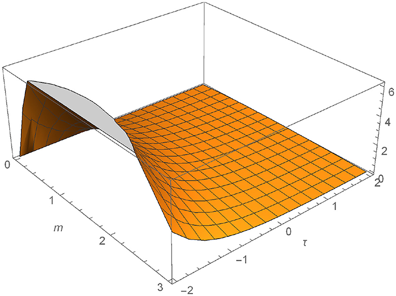
Figure 1. Graphical representation of M defined in Equation (13) for ω = 0.8.

Figure 2

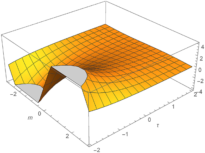
Figure 2. Graphical representation of M defined in Equation (13) for ω = 1.

Figure 3

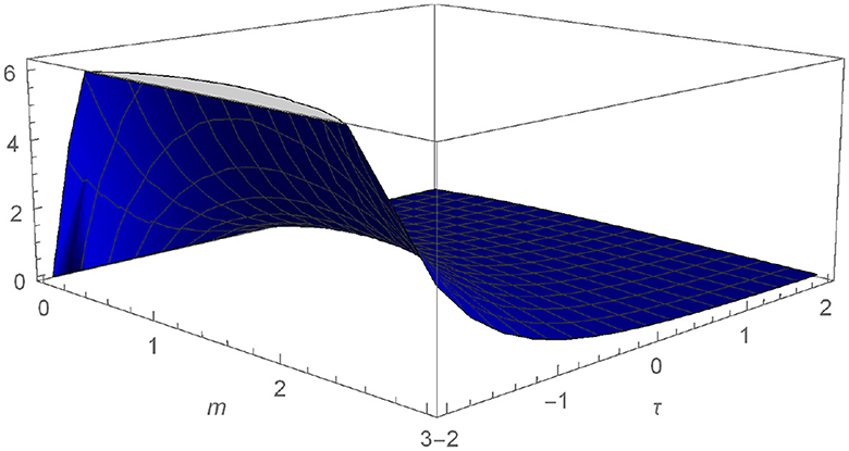
Figure 3. Graphical representation of N defined in Equation (14) for ω = 0.8.

Figure 4

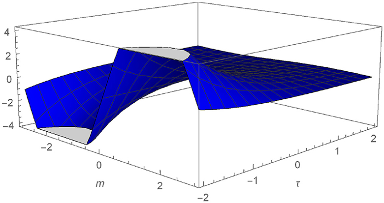
Figure 4. Graphical representation of N defined in Equation (14) for ω = 1.

6 Conclusions

In this study, a strategy that combines the Elzaki-transform and Adomian-decomposition approaches is used. We made an effort to show the effectiveness of the recommended strategy. The objective of this study is to resolve the coupled Burger equation. The illustration depicts the proposed method's applicability. Visual representations of the solution show how the method applies to generalized non-linear equations. Plots with various values of ω are used to illustrate the solutions that were found during the inquiry. Elzaki decomposition is a powerful, quick, and effective approach to solving the local fractional non-linear coupled Burger equation, as we have discovered.

Data availability statement

The original contributions presented in the study are included in the article/supplementary material, further inquiries can be directed to the corresponding author.

Author contributions

GA: Funding acquisition, Resources, Visualization, Writing—review & editing. JP: Conceptualization, Investigation, Methodology, Writing—original draft. BA: Data curation, Formal analysis, Project administration, Writing—review & editing. RD: Software, Supervision, Validation, Writing—original draft.

Funding

The author(s) declare financial support was received for the research, authorship, and/or publication of this article. This work was supported and funded by the Deanship of Scientific Research at Imam Mohammad Ibn Saud Islamic University (IMSIU; grant number: IMSIU-RP23066).

Acknowledgments

We would like to express our sincere thanks to the editor and reviewers for their valuable comments and suggestions. The authors thank the Dean of Scientific Research at Imam Mohammad Ibn Saud Islamic University for their support.

Conflict of interest

The authors declare that the research was conducted in the absence of any commercial or financial relationships that could be construed as a potential conflict of interest.

Publisher's note

All claims expressed in this article are solely those of the authors and do not necessarily represent those of their affiliated organizations, or those of the publisher, the editors and the reviewers. Any product that may be evaluated in this article, or claim that may be made by its manufacturer, is not guaranteed or endorsed by the publisher.

References

1. Oldham KB, Spanier J. The Fractional Calculus: Theory and Applications of Differentiation and Integration to Arbitrary Order, Vol. 11 of Mathematics in Science and Engineering. New York, NY: Academic Press (1974).

Google Scholar

2. Miller KS, Ross B. An Introduction to the Fractional Calculus and Fractional Differential Equations. A Wiley-Interscience Publication. New York, NY: John Wiley and Sons (1993).

Google Scholar

3. Podlubny I. Fractional Differential Equations. Vol. 198 of Mathematics in Science and Engineering. San Diego, CA: Academic Press (1999).

Google Scholar

4. Srivastava HM, Owa S. Univalent functions, Fractional Calculus and Their Applications. New York, NY: Halsted Press/Wiley (1989).

Google Scholar

5. Singh H, Srivastava HM, Hammouch, Z, Nisar KS. Numerical simulation and stability analysis for the fractional-order dynamics of COVID-19. Result Phys. (2021) 20:103722. doi: 10.1016/j.rinp.2020.103722

PubMed Abstract | Crossref Full Text | Google Scholar

6. Kilbas AA, Srivastava HM, Trujillo JJ. Theory and Applications of Fractional Differential Equations. North-Holland Mathematics Studies, 204. Amsterdam: Elsevier Science B.V. (2006).

Google Scholar

7. Gdawiec K, Qureshi, IK, Qureshi, S, Soomro, A. An optimal homotopy continuation method: convergence and visual analysis. J Comput Sci. (2023) 74:102166. doi: 10.1016/j.jocs.2023.102166

Crossref Full Text | Google Scholar

8. Abdulganiy R, Ramos H, Adekunle OJ, Okunga SA. A functionally-fitted block hybrid Falkner method for Kepler equations and related problems. Comput Appl Math. (2023) 42:327. doi: 10.1007/s40314-023-02463-y

Crossref Full Text | Google Scholar

9. Onder I, Esen H, Secer A, Ozisik M. Stochastic optical solitons of the perturbed nonlinear Schrodinger equation with Kerr law via lto calculus. Eur Phys J Plus. (2023) 138:1–12. doi: 10.1140/epjp/s13360-023-04497-x

Crossref Full Text | Google Scholar

10. Zafar ZUA, Yusuf A, Musa SS, Qureshi S, Alshomrani AS, Balenau D. Impact of public health awareness programs on COVID-19 dynamics: a fractional modeling approach. Fractals. (2022) 2022:S0218348X23400054. doi: 10.1142/S0218348X23400054

Crossref Full Text | Google Scholar

11. Sharma S, Goswami, P, Baleanu D, Dubey RS. Comprehending the model of omicron variant using fractional derivatives. Appl Math Sci Eng. (2022) 31:2159027. doi: 10.1080/27690911.2022.2159027

Crossref Full Text | Google Scholar

12. Barbosa RS, Machado JAT, Ferreira IM. PID controller tuning using fractional calculus concepts. Fract Calc Appl Anal. (2004) 7:119–34. doi: 10.1115/DETC2003/VIB-48375

Crossref Full Text | Google Scholar

13. Saadeh R, Ahmed SA, Qazza A, Elzaki TM. Adapting partial differential equations via the modified double ARA-Sumudu decomposition method. Part Diff Eq Appl Math. (2023) 8:100539. doi: 10.1016/j.padiff.2023.100539

Crossref Full Text | Google Scholar

14. Machado JAT. Analysis and design of fractional-order digital control systems. Syst Anal Model Simul. (1997) 27:107–22.

Google Scholar

15. Momani S. Analytical approximate solution for fractional heat-like and wave-like equations with variable coefficients using the decomposition method. Appl. Math. Comput. (2005) 165:459–72. doi: 10.1016/j.amc.2004.06.025

Crossref Full Text | Google Scholar

16. Althobaiti S, Dubey RS, Prasad JG. Solution of local fractional generalized Fokker-Planck equation using local fractional mohand adomian decomposition method. Fractals. (2021) 30:1–9. doi: 10.1142/S0218348X2240028X

Crossref Full Text | Google Scholar

17. Saadeh R, Qazza A, Burqan A, Al-Omari S. On time fractional partial differential equations and their solution by certain formable transform decomposition method. Comput Model Eng Sci. (2023) 136:3121–39. doi: 10.32604/cmes.2023.026313

Crossref Full Text | Google Scholar

18. Albalawia, KS, Shokhandab R, Goswami P. On the solution of generalized time-fractional telegraphic equation. Appl Math Sci Eng. (2023) 31:1. doi: 10.1080/27690911.2023.2169685

Crossref Full Text | Google Scholar

19. Momani S, Odibat Z. Analytical solution of a time-fractional Navier–Stokes equation by Adomian decomposition method. Appl Math Comput. (2006) 177:488–94. doi: 10.1016/j.amc.2005.11.025

Crossref Full Text | Google Scholar

20. Jafari H, Prasad JG, Goswami P, Dubey RS. Solution of the local fractional generalized KDV equation using homotopy analysis method. Fractal. (2021) 29:5. doi: 10.1142/S0218348X21400144

Crossref Full Text | Google Scholar

21. Alquran M, Ali M, Gharaibeh F, Qureshi S. Novel investigation of dual-wave solutions to the Kadomtsev-Petviashvili model involving second-order temporal and spatial-temporal dispersion terms. Part Diff Eq Appl Math. (2023) 8:100543. doi: 10.1016/j.padiff.2023.100543

Crossref Full Text | Google Scholar

22. Qureshi S, Akanbi MA, Shaikh AA, Wusu AS, Ogunlaran OM, Mahmoud W, et al. A new adaptive nonlinear numerical method for singular and stiff differential problems. Alexand Eng J. (2023) 74:585–97. doi: 10.1016/j.aej.2023.05.055

Crossref Full Text | Google Scholar

23. Ilhan Ö, Sahin G. A numerical approach for an epidemic SIR model via Morgan-Voyce series. Int J Math Comput Eng. (2024) 2:123–38. doi: 10.2478/ijmce-2024-0010

Crossref Full Text | Google Scholar

24. Erdogan F. A second order numerical method for singularly perturbed Volterra integro differential equations with delay. Int J Math Comput Eng. (2024) 2:85–96. doi: 10.2478/ijmce-2024-0007

Crossref Full Text | Google Scholar

25. Nasir M, Jabeen S, Afzal F, Zafar A. Solving the generalized equal width wave equation via sextic B-spline collocation technique. Int J Math Comput Eng. (2023) 1:229–42. doi: 10.2478/ijmce-2023-0019

Crossref Full Text | Google Scholar

26. Ziane D. Cherif MH, Cattani C, Belghaba K. Yang-Laplace decomposition method for nonlinear system of local fractional partial differential equations. Appl Math Nonlin Sci. (2019) 4:489–502. doi: 10.2478/AMNS.2019.2.00046

Crossref Full Text | Google Scholar

27. Ziane D, Baleanu D, Belghaba K, Cherif MH. Local fractional Sumudu decomposition method for linear partial differential equations with local fractional derivative. J King Saud Univ Sci. (2019) 31:83–8. doi: 10.1016/j.jksus.2017.05.002

Crossref Full Text | Google Scholar

28. He JH, Wu GC, Austin F. The variational iteration method which should be followed. Nonlin Sci Lett A. (2010) 1:1–30. doi: 10.4236/oalib.1106601

Crossref Full Text | Google Scholar

29. Momani S, Odibat Z, Alawneh A. Variational iteration method for solving the space and time-fractional KdV equation. Numer Methods Part Diff Eq. (2008) 24:262–71. doi: 10.1002/num.20247

Crossref Full Text | Google Scholar

30. Maitama S, Zhao W. Local fractional homotopy analysis method for solving non-differentiable problems on Cantor sets. Adv Diff Eq. (2019) 127:22. doi: 10.1186/s13662-019-2068-6

Crossref Full Text | Google Scholar

31. Liao SJ. The Proposed Homotopy Analysis Technique for the Solution of Nonlinear Problems, (Ph.D. thesis), Shanghai Jiao Tong University, Shanghai, China (1992).

Google Scholar

32. Zhao Z, Li C. Fractional difference/finite element approximations for the time-space fractional telegraph equation. Appl Math Comput. (2012) 219:2975–88. doi: 10.1016/j.amc.2012.09.022

Crossref Full Text | Google Scholar

33. Burgers JM. A mathematical model illustrating the theory of turbulence. Adv Appl Mech. (1948) 1:171–99.

Google Scholar

34. Esipov SE. Coupled Burgers' equations: a model of polydispersive sedimentation. Phys Rev E. (1995) 52:3711–8.

PubMed Abstract | Google Scholar

35. Rashid A, Ismail AIBM. A fourier pseudospectral method for solving coupled viscous Burgers equations. Comput Methods Appl Math. (2009) 9:412–20. doi: 10.2478/cmam-2009-0026

Crossref Full Text | Google Scholar

36. Islam SU, Haq S, Uddin M. A meshfree interpolation method for the numerical solution of the coupled nonlinear partial differential equations. Eng Anal Bound Elem. (2009) 33:399–409. doi: 10.1016/j.enganabound.2008.06.005

Crossref Full Text | Google Scholar

37. Alqahtani AM, Prasad JG. Solution of local fractional generalized coupled Korteweg–de vries (cKdV) equation using local fractional homotopy analysis method and Adomian decomposition method. Appl Math Sci Eng. (2024) 32:1. doi: 10.1080/27690911.2023.2297028

Crossref Full Text | Google Scholar

38. Kumar M, Pandit S. A composite numerical scheme for the numerical simulation of coupled Burgers' equation. Comput Phys Commun. (2014) 185:809–17. doi: 10.1016/j.cpc.2013.11.012

Crossref Full Text | Google Scholar

39. Mohammadi M, Mokhtari R. A reproducing kernel method for solving a class of nonlinear systems of pdes. Math Model Anal. (2014) 19:180–98. doi: 10.3846/13926292.2014.909897

Crossref Full Text | Google Scholar

40. Bak S, Kim P, Kim D. A semi-Lagrangian approach for numerical simulation of coupled Burgers' equations. Commun Nonlin Sci Numer Simul. (2019) 69:31–44. doi: 10.1016/j.cnsns.2018.09.007

Crossref Full Text | Google Scholar

41. Anac H. A local fractional elzaki transform decomposition method for the nonlinear system of local fractional partial differential equations. Fractal Fraction. (2022) 6:167. doi: 10.3390/fractalfract6030167

Crossref Full Text | Google Scholar

42. Tarig E, Elzaki SM. Application of new transform “Elzaki Transform” to partial differential equations. Glob J Pure Appl Math. (2011) 7:65–70. doi: 10.3390/fractalfract6030167

Crossref Full Text | Google Scholar

43. Dubey RS, Goswami P, Gomati AT. A new analytical method to solve Klein-Gordon equations by using homotopy perturbation Mohand transform method. Malaya J Matematik. (2022) 10:1. doi: 10.26637/mjm1001/001

Crossref Full Text | Google Scholar

44. Ige OE, Oderinu RA, Elzaki TM. Adomian polynomial and Elzaki transform method for solving Sine-Gordon equations. IAENG Int J Appl Math. (2019) 49:344–50. doi: 10.12732/ijam.v32i3.7

Crossref Full Text | Google Scholar

45. Yang XJ. Local Fractional Calculus and Its Applications. New York, NY: World Science Publisher (2012).

PubMed Abstract | Google Scholar

46. Yang AM, Zhang YZ, Cattani C, Xie GN, Rashidi MM, Zhou YJ, et al. Application of local fractional series expansion method to solve Klein–Gordon equations on Cantor sets. Abstr Appl Anal. (2014) 2014:7. doi: 10.1155/2014/372741

Crossref Full Text | Google Scholar