Analyzing cooperative game theory solutions: core and Shapley value in cartesian product of two sets

1 Introduction

Mathematical modeling plays a crucial role in solving real-life problems across various fields such as engineering [1, 2], biology [3, 4], economics [5, 6], and many others. In this study, the example of an agreement between a company and three adjacent villages to provide electricity and water services will be predominantly utilized. To simplify the calculations, it is assumed that the project would cost 50 million for water and 50 million for electricity if the company was undertaken these services separately. For geographical reasons, the project manager proposes reduced costs of (80;80), (85;85), and (90;90), respectively, for common contracts between the first village and the second, the first village and the third, and the second village and the third. Furthermore, there is a comprehensive contract that includes all three villages, and its total cost is (80;80;80). The question that arises is the following. How do we choose the best collaboration?

When addressing such scenarios, individuals often arrive at various conclusions. Some may contend that a multitude of potential agreements exist, while others may argue that no stable agreement is possible. Alternatively, some emphasize the potential for a unique cooperative solution in fairly general contexts. Cooperative game theory provides solution concepts for this type of problem, such as the core and the Shapley value. These concepts address issues related to the distribution of costs or gains, decision-making power, and more. They are grounded in criteria that encompass rationality and equity considerations [7–11]. Game theory has garnered significant attention in numerous scholarly articles and publications [12–15], and in the past few years, many researchers have extended the concept of cooperative games. To illustrate, in 2000, a new class of cooperative games was introduced by Bilbao et al. [16] known as bi-cooperative games. The authors introduced this notion as the generalization of cooperative games, which refers to situations in which each player can participate positively, negatively, or not at all. That is the coalition function is defined over the pairs (S, T) of disjoint coalitions, where the members of S are positive contributors and members of T are negative contributors.

In 2008, Bilbao et al. [17] provided an axiomatic characterization of the Shapley value in the context of bi-cooperative games. Since then, this theory has garnered considerable attention within scholarly circles, which is evidenced by numerous publications such as the study conducted by Wu et al. [18]. Their study delved into unique characterizations for bi-cooperative games, with a particular emphasis on the Shapley value, introducing distinct properties and exploring alternative axiomatizations. Notably, they proposed a one-point solution concept, alongside fundamental axioms such as linearity and efficiency. Furthermore, Abbas [19] contributed significantly to this field by extending the co-Möbius transform of cooperative games to bi-cooperative games, thereby introducing the concept of the bipolar co-Möbius transform. This extension enriches the theoretical framework, opening avenues for deeper analysis and understanding. Additional pertinent references include the studies mentioned in the references Bilbao et al. [20], Borkotokey et al. [21], and Doménech et al. [22]. Concurrently, Puerto et al. [23] introduced another class of cooperative games whose characteristic function ranges on any linear space. In this study, the authors extended the nature of the payoffs rather than imposing conditions on the argument of the characteristic function. This approach facilitated subsequent research endeavors by various scholars, with notable contributions cited in references such as Branzei et al. [24] Gök et al. [25], Branzei et al. [26], and Nan et al. [27], among others.

To summarize, Puerto et al. introduced partially ordered cooperative games utilizing functions defined from 2^N∪{∅} to ℵ, while Bilbao et al. introduced bi-cooperative games employing functions defined from 3^N to ℝ. Although both approaches employ a single game, it might be more advantageous to adopt a high-dimensional approach depending on the nature of the problem, as this approach could better express and reflect the complexities of the problem beyond a one-dimensional representation. Consequently, our analysis takes a distinct route by exploring cooperative scenarios where players make choices on the cartesian product N × N′. Our functions are defined from 2^{N × N}′ to ℝ, aiming to offer a fresh perspective to game theory by leveraging the cartesian product of two sets. Figure 1 visually depicts the evolution from cooperative games to bi-cooperative games within a single set, partially ordered games, and to bi-dimensional cooperative games across the cartesian product of two sets.

Figure 1

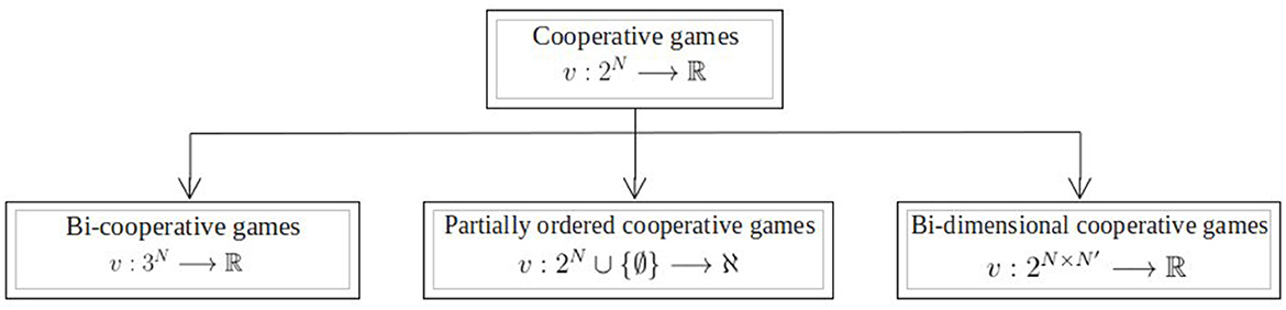
Figure 1. Evolution of cooperative games.

In this enriched framework, a coalition is a list of pairs of actions, one pair for each player of this coalition. As usual, a player's payoff in a game is a real number that represents what that player can expect when he agrees to participate in the game. Within this framework, the notion of rationality in the cartesian product of two sets N and N′ (individual rationality and coalitional rationality) is employed, rather than rationality solely in N to define the set of imputations and the core which is the set of acceptable arbitration. It is important to mention that while this set offers valuable insights into the sharing problem, it might not invariably yield a conclusive solution, as highlighted in remark 2.3.3. Therefore, the Shapley value is introduced as another essential solution concept. By incorporating this concept and applying it to the illustrative example mentioned earlier, a unique and definitive solution has been successfully identified.

This study is organized as follows. In the next section, some materials and methods of cooperative game in N × N′ are given. In Section 3, an axiomatic characterization of the Shapley value in terms of efficiency, symmetry, null player, and additivity is provided using the coalition A*B. Moreover, the last section concludes the article.

2 Materials and methods

2.1 Cooperative game in N × N′

In this paragraph, the classical notions of cooperative game in N × N′ that will be used in this study are defined.

Definition 2.1.1. A coalition A × B is defined as a subset of N × N′, and the set of all coalitions is the set 2^{N × N}′ of cardinal 2^nm. With |N| = n and |N′| = m.

By convention, the empty set can also be designated as a coalition, referred to as the empty coalition. The set N × N′ is also a coalition, known as the grand coalition.

Definition 2.1.2. A cooperative game on N × N′ is defined by a finite set of pairs of players

$N\times N^{\prime }=\left\{(a_i;b_j),a_i\in N,b_j\in N^{\prime }\mathrm{\text{and}}(i;j)\in \left\{1;2;...;n\right\}\times \left\{1;2;...;m\right\}\right\}$, and a real-valued v, defined on all subsets of N × N′, (with v(∅) = 0).

Remark 2.1.1. Drawing an analogy to von Neumann and Morgenstern's work in Roth's book [28], we stipulate that v must be superadditive, i.e., if A × A′ and B × B′ are two disjoint subsets of N × N′, v[(A × A′)⊔(B × B′)] ≥ v(A × A′)+v(B × B′), where (A × A′)⊔(B × B′) designates the disjoint reunion of (A × A′) and (B × B′). This implies that the value of the coalition (A × A′)⊔(B × B′) is no less than the aggregate value of its individual parts acting independently.

Definition 2.1.3. A dual game in N × N′ of the cooperative game v is the function denoted by v^× defined by,

$\begin{array}{l}{v}^{\times }:2^{N\times N^{\prime }}\to {ℝ}^{+}\\ (A\times A^{\prime })\mapsto v(N\times N^{\prime })-v\left[{(A\times A^{\prime })}^c\right]\end{array}$

Corollary 2.1.1. Let v be a cooperative game in N × N′. The following properties are observed:

1. v is an increasing function on 2^{N × N}′.

2. v^× is an increasing function on 2^{N × N}′.

Proof:

Let (A × A′) and (B × B′) be two elements of 2^{N × N}′.

1. If A × A′⊂B × B′, then, B × B′ = (A × A′)⊔(B × B′\A × A′) and (A × A′)∩(B × B′\A × A′) = ∅, [29, 30], therefore,

$\begin{array}{l}v(B\times B^{\prime })=v[(A\times A^{\prime })\bigsqcup (B\times B^{\prime }\backslash A\times A^{\prime })]\\ \ge v(A\times A^{\prime })+v(B\times B^{\prime }\backslash A\times A^{\prime })\\ \ge v(A\times A^{\prime }).\end{array}$

   Since we have

$A\times A^{\prime }\subset B\times B^{\prime }\Rightarrow v(A\times A^{\prime })\le v(B\times B^{\prime }),$

   v is an increasing function.

2. We suppose that A × A′⊂B × B′, then

$\begin{array}{l}{v}^{\times }(A\times A^{\prime })=v(N\times N^{\prime })-v\left[{(A\times A^{\prime })}^c\right]\\ \le v(N\times N^{\prime })-v\left[{(B\times B^{\prime })}^c\right]\\ \le v^{\times }(B\times B^{\prime }).\end{array}$

   Hence, v^× is an increasing function.

Definition 2.1.4. The particular coalition A*B is defined as follows:

$A*B=\left\{(a_i;b_i),a_i\in A,b_i\in B\text{and}i\in \left\{1;2;...;p\right\}\right\}.$

The coalition N*N′ will be defined as follows:

$N*N^{\prime }=\left\{(a_i;b_i),a_i\in N,b_i\in N^{\prime }\text{and}i\in \left\{1;2;...;n\right\}\right\}.$

Notations:

1. The worth for a player i will be denoted by v(a_i; b_i).

2. The worth of the coalition A*B will be denoted by v(A*B).

3. The payoff that each player i receives will be denoted by x_i.

4. The vector x = (x₁; x₂; ...;x_p) is called allocation or payoff rule of game.

Remark 2.1.2. The focus will be on the A * B coalitions. Assuming that p players convene simultaneously in two games, A and B, under the leadership of a representative who offers each player i a weighted share of the payoff denoted by x_i. Consequently, the cardinality of A * B will be p if the coalition comprises p players.

For unanimous agreement, it is imperative that x_i ≥ v(a_i; b_i) holds true for all i in 1;2;...;p. This ensures that player i cannot be incentivized to join a coalition by offering them less than what they would earn individually.

Example:

The “cost allocation” problem discussed in the introduction can be clarified through a cooperative game involving three players within the framework of N × N′. The first game represents the electricity component, denoted as (E), while the second pertains to the water component, designated as (W). The worth of a coalition is determined by the total cost saving between water and electricity. Hence, we have v(E₁ * W₁) = 0, v(E₂ * W₂) = 0, v(E₃ * W₃) = 0, v(E₁ * W₁ ⊔ E₂ * W₂) = 40, v(E₁ * W₁ ⊔ E₃ * W₃) = 30, v(E₂ * W₂ ⊔ E₃ * W₃) = 20, and v(E * W) = 60.

In this game, it is observed that the sum of the worths of two disjoint coalitions is always less than or equal to the worth resulting from their cooperation. Therefore, this game is necessarily cooperative.

Proposition 2.1.1. Let x be a payoff rule of cooperative game v, then, ∀i ∈ {1;2;...;n}, x_i ≥ 0. (i.e., the payoffs of all players are non-negative).

Proof:

Suppose that v is a cooperative game, v is monotonic increasing function.

We know that v(∅) = 0 and since ∅ ⊂ A * B for all subset A * B of N * N′, then v(A * B) ≥ 0 for all A * B, (i.e. v ≥ 0).

Since x_i ≥ v for all i ∈ {1;2;...;p}, then x_i ≥ 0 for all i.

Definition 2.1.5. A game is called efficiency if, $v(N*N^{\prime })={\displaystyle \sum _{i=1}^n}{x}_i.$ (i.e., the worth of the grand coalition is completely shared among all players).

Definition 2.1.6. Let v be a cooperative game, and let (a_i; b_i), (a_j; b_j) ∉ A * B.

Two players i and j are symmetric if v(A * B ⊔ {(a_i; b_i)}) = v(A * B ⊔ {(a_j; b_j)}). (i.e., i and j both contribute equally to every coalition that does not include them).

Proposition 2.1.2. Let i and j be two symmetric players. Then, x_i = x_j. (i.e., their payoffs coincide).

Proof:

If i and j are symmetric players, the worth of A * B ⊔ {(a_i; b_i)} and the worth of A * B ⊔ {(a_j; b_j)} are the same, with (a_i; b_i), (a_j; b_j) ∉ A * B.

Therefore, the worth for player i is equal to the worth for player j (i.e., v({(a_i; b_i)}) = v({(a_j; b_j)})).

Since the share of the payoffs is weighted, x_i = x_j.

Definition 2.1.7. Let v be a cooperative game, and let (a_i; b_i) ∉ A * B.

Player i is called dummy player if, v(A * B ⊔ {(a_i; b_i)}) = v(A * B) + v({(a_i; b_i)}). (i.e., i only contributes its own worth to every coalition).

Proposition 2.1.3. If i be a dummy player, v({(a_i; b_i)}) = x_i (i.e., the worth and the payoff of player i coincides).

Proof:

Let v be a cooperative game and suppose that (a_i; b_i) ∉ A * B.

v(A * B ⊔ {(a_i; b_i)}) = v(A * B) + v({(a_i; b_i)}) mean that the gain that player i receives with the coalition A*B is the same when player i plays alone, we necessarily have x_i = v({(a_i; b_i)}).

Definition 2.1.8. Let v be a cooperative game.

The player i is called a null player if v(A * B ⊔ {(a_i; b_i)}) = v(A * B), with (a_i; b_i) ∉ A*B, (i.e., its presence or deletion has no effect on the worth of every coalition).

Proposition 2.1.4. If i is a null player, x_i = 0 (i.e. its payoff is zero).

Proof:

This is a particular case of dummy player property.

Proposition 2.1.5. Let v and w be two cooperative games. Let x be a payoff rule. Then, we have x_i(v + w) = x_i(v) + x_i(w) for all i. (i.e., the individual payoff of a game defined as the sum of two games coincides with the addition of the individual payoffs of these two games).

2.2 Marginal contribution–convex game

In this paragraph, the marginal contribution and convex games in N * N′ will be defined. (Some references used [31–35]).

Definition 2.2.1. Let v be a cooperative game. The marginal contribution of player i to the coalition A * B being defined by c_i(A * B) = v(A * B ⊔ {(a_i; b_i)})−v(A * B), with (a_i; b_i) ∉ A * B.

In other words,

the value c_i(A * B) is the amount from which player i cannot be prevented from when the complement A * B receives v(A*B).

Example:

The worth of v^× (the dual game) can be interpreted as indicating the marginal contribution of coalition A * B to the coalition N * N′.

Proposition 2.2.1. Let v be a cooperative game.

1. If i and j are symmetric, c_i(A * B) = c_j(A * B) (i.e., their marginal contributions coincide).

2. If i is a dummy player, c_i(A * B) = v({(a_i; b_i)}) (i.e., its marginal contribution equals its worth).

3. If i is a null player, c_i(A * B) = 0 (i.e., its marginal contribution is null).

Proof:

1. Suppose that i and j are symmetric.

   If (a_i; b_i), (a_j; b_j) ∉ A * B, v(A * B ⊔ {(a_i; b_i)}) = v(A * B⊔{(a_j; b_j)}).

   Hence, c_i(A * B) = c_j(A * B).

2. Suppose that i is a dummy player, v(A * B ⊔ {(a_i; b_i)}) = v(A * B) + v({(a_i; b_i)}); therefore, v(A * B ⊔ {(a_i; b_i)})−v(A * B) = v({(a_i; b_i)}). Hence, c_i(A * B) = v({(a_i; b_i)}).

3. Suppose that i is a null player, v(A * B⊔{(a_i; b_i)}) = v(A * B); therefore, v(A * B⊔{(a_i; b_i)})−v(A * B) = 0. Hence, c_i(A * B) = 0.

Definition 2.2.2. A cooperative game v is convex if for all parts A * A′ and B * B′ in N * N′, we have

$v(A*A^{\prime })+v(B*B^{\prime })\le v\left[(A*A^{\prime })\cup (B*B^{\prime })\right]+v\left[(A*A^{\prime })\cap (B*B^{\prime })\right].$

Remark 2.2.1. It is clear that a convex game is cooperative. Because in a cooperative game, we suppose that (A * A′) ∩ (B * B′) = ∅.

Proposition 2.2.2. Suppose that A * B ⊂ A′ * B′ and $(a_i;b_i)\notin A^{\prime }*B^{\prime }$. A game v is convex if $v(A*B\bigsqcup \left\{(a_i;b_i)\right\})-v(A*B)\le v(A^{\prime }*B^{\prime }\bigsqcup \left\{(a_i;b_i)\right\})-v(A^{\prime }*B^{\prime })$.

In other words,

the game v is convex if $c_i(A*B)\le c_i(A^{\prime }*B^{\prime })$, with A * B ⊂ A′*B′ (i.e., the marginal contribution of a player i is increasing in the sense of inclusion).

Proof:

Let A * B and A′ * B′ be two subsets of N * N′ such that A * B ⊂ A′ * B′ and $(a_i;b_i)\notin A^{\prime }*B^{\prime }$, then

$(A*B\bigsqcup \left\{(a_i;b_i)\right\})\cap (A^{\prime }*B^{\prime })=A*B$.

v is convex

$\begin{array}{l}\iff v(A*B\bigsqcup \{(a_i;b_i)\})+v(A^{\prime }*B^{\prime })\le v[(A*B\bigsqcup \{(a_i;b_i)\}){{\displaystyle \cup }}^{\text{}}(A^{\prime }*\\ B^{\prime })]+v[(A*B\bigsqcup \{(a_i;b_i)\}){{\displaystyle \cap }}^{\text{}}(A^{\prime }*B^{\prime })]\\ \iff v(A*B\bigsqcup \{(a_i;b_i)\})+v(A^{\prime }*B^{\prime })\le v(A^{\prime }*B^{\prime }\bigsqcup \{(a_i;b_i)\})+v(A*B)\\ \iff v(A*B\bigsqcup \{(a_i;b_i)\})-v(A*B)\le v(A^{\prime }*B^{\prime }\bigsqcup \{(a_i;b_i)\})-v(A^{\prime }*B^{\prime })\\ \iff c_i(A*B)\le c_i(A^{\prime }*B^{\prime }).\end{array}$

Remark 2.2.2. Convex games appear in several applications of game theory. For example, Monopoly Firm, Trading Game, and Aircraft Landing Fee Game [36].

2.3 Rationality–imputation–core

Definition 2.3.1. Let x be a payoff rule of the cooperative game v.

We say that players' thinking is rational if ∀i ∈ {1;2;...;n}, x_i≥v(a_i; b_i) (i.e., the payoff of every player has to be at least its worth).

Definition 2.3.3. Let v be a cooperative game.

The set of imputations of v is the set of individually rational utilities attainable for the grand coalition

$𝕀=\left\{x\in {ℝ}^n,{\displaystyle \sum _{i=1}^n}{x}_i=v(N*N^{\prime })\text{and}\forall i\in \left\{1;2;...;n\right\},x_i\ge v(a_i;b_i)\right\}.$

Remark 2.3.1. Notice that superadditive games have a non-empty set of imputations. The n players acting together can win exactly v(N * N′), and sharing such as ${\displaystyle \sum _{i=1}^n}{x}_i<v(N*N^{\prime })$ will therefore not be accepted, as this amounts to wasting the quantity $v(N*N^{\prime })-{\displaystyle \sum _{i=1}^n}{x}_i$.

The first criterion for acceptable arbitration remains insufficient; hence, introducing a second criterion becomes necessary. The concept is to replace individual rationality with coalition rationality, a more stringent condition. This transition brings forth the subsequent definition.

Definition 2.3.3. Let x be a payoff rule of the cooperative game v. The reasoning of players within the coalition A * B is deemed rational if ${\displaystyle \sum _{i=1}^p}{x}_i\ge v(A*B)$, with A * B⊂N * N′ and |A * B| = p (i.e., the payoff that the coalition A * B obtains has to be at least its worth).

Remark 2.3.2. Notice that ${\displaystyle \sum _{i=1}^p}{x}_i\ge v(A*B)$ implies that for all i ∈ {1;2;...;p}, x_i≥v(a_i; b_i), with (a_i; b_i) ∈ A * B and |A * B| = p.

Indeed, if there exists i ∈ {1;2;...;p} such that x_i ≤ v(a_i; b_i), player i would not agree to join this coalition.

Definition 2.3.4. Let A * B be a coalition containing p players.

An imputation x ∈ ℝ^p is considered blocked by the coalition A * B if there exists a vector represented by x^{A * B} in ℝ^p such that,

$\forall i\in \{1;2;\mathrm{...};p\},x_i^{A*B}\ge x_i \text{and} {\displaystyle \sum _{i=1}^p{x}_i^{A*B}=v(A*B).}$

Example:

In our game “cost allocation,” if the imputation x = (15;15;30) is proposed, i.e., if the three villages pay respectively 85, 85, and 70, the coalition E₁ * W₁ ⊔ E₂ * W₂ may oppose this sharing because x₁+x₂ = 30 while v(E₁ * W₁ ⊔ E₂ * W₂) = 40. Otherwise, we can propose the imputation x = (20;20;20), which is better for each of its members because x₁+x₂ = 40 = v(E₁ * W₁ ⊔ E₂ * W₂), x₁+x₃ = 40≥30 = v(E₁ * W₁ ⊔ E₃ * W₃), and x₂+x₃ = 40≥20 = v(E₂ * W₂ ⊔ E₃ * W₃). It is also achievable because x₁+x₂+x₃ = 60 = v(E * W). It is then asserted that E₁ * W₁ ⊔ E₂ * W₂ prefers (20;20;20) to (15;15;30). Therefore, the imputation (15;15;30) is dominated because it is blocked by E₁ * W₁ ⊔ E₂ * W₂.

Eliminating all dominated imputations effectively eradicates any potential for group disputes and establishes the core of the game, which is defined as the collection of imputations that are not dominated. Definition 0.0.0.15.

The core of the game is defined as the set of imputations that are not blocked by any coalition. Therefore, the core of v corresponds to the payoff rule x given as follows:

$ℂ=\{x\in {ℝ}^n,{\displaystyle \sum _{i=1}^n}{x}_i=v(N*N^{\prime })$

$\text{and}{\displaystyle \sum _{i=1}^{|A*B|}}{x}_i\ge v(A*B);A*B\subset N*N^{\prime }\}.$

In other words,

the core of the game is the set of acceptable arbitration. If the arbiter proposes an imputation x which is not in the core, the players of A * B will refuse it.

Example:

For the “cost allocation” example, an allocation (x₁; x₂; x₃) is therefore in the core if x₁ ≥ 0, x₂ ≥ 0, x₃ ≥ 0, x₁ + x₂ ≥ v(E₁ * W₁⊔E₂ * W₂) = 40, x₁ + x₃ ≥ v(E₁ * W₁⊔E₃ * W₃) = 30, x₂ + x₃ ≥ v(E₂ * W₂⊔E₃ * W₃) = 20, and x₁ + x₂+x₃ = v(E * W) = 60.

Remark 2.3.3. Noticeably, several sharing proposals satisfy these conditions, including (20;20;20), (40;20;0), (30;30;0), or (40;0;20). Thus, a unique solution is not provided. The core can be infinite or empty or reduced to a single point. In other words, this set does not always provide a definitive solution to the sharing problem, and if it is empty, it does not offer any help to players in knowing their respective payoffs.

The results like those of Bondareva [31] and Shapley [32] have identified other classes of games where the core is never empty. One of these classes is the case of convex games.

3 The Shapley value in N * N′

As discussed in paragraph 2.3, under remark 2.3.3, it became evident that the concept of a core does not offer (in general) a singular resolution to sharing problems. In light of this, we now introduce the Shapley value that assigns a distinct payoff vector to each game. In this paragraph, the existence and uniqueness of the Shapley value in N * N′ will be proven.

3.1 The Shapley axioms

The value of player i in the cooperative game v is denoted by ϕ_i(v).

A value function ϕ = (ϕ₁(v);ϕ₂(v);...;ϕ_n(v)) is a function that assigns to each possible characteristic function of an n-person game.

The ith component of the n-tuple may be considered as a power of the ith player in the game, and the value vector can be considered as an arbitration result of the game decided by a fair arbiter.

The Shapley value is introduced axiomatically, following the same principles as the classical Shapley value in N [28, 37–42]. The four Shapley axioms in N * N′ can be described as follows:

1. Efficiency: $v(N*N^{\prime })={\displaystyle \sum _{i=1}^n}{\varphi }_i(v)$, (i.e., the solution should distribute the maximal total payoff).

2. Symmetry: If v(A * B⊔{(a_i; b_i)}) = v(A * B⊔{(a_j; b_j)}), with(a_i; b_i), (a_j; b_j)∉A * B, then ϕ_i(v) = ϕ_j(v) (i.e., any two players who contribute the same input should obtain the same payoff).

3. Null player: If v(A * B⊔{(a_i; b_i)}) = v(A * B), with (a_i; b_i)∉A * B, ϕ_i(v) = 0 (i.e., any player who contributes nothing to any coalition should obtain nothing).

4. Additivity: ϕ(v+w) = ϕ(v)+ϕ(w) (i.e., adding the solution of two games together solves the sum of these games).

Theorem 3.1.1. There exists a unique function ϕ satisfying the Shapley axioms.

Proof:

Existence:

Let A * B be a non-empty subset of N * N′. Let W_{A * B} defined for all A′ * B′ in 2^{N × N}′ by

$\begin{array}{ll}{W}_{A\ast B}(A^{\prime }\ast B^{\prime })=\{\begin{array}{l}1\text{\hspace{1em}\hspace{1em}if }A\ast B\subset A^{\prime }\ast B^{\prime }\\ 0\text{\hspace{1em}\hspace{1em}otherwise}.\end{array}& (1)\end{array}$

We have $W_{A*B}(N*N^{\prime })=1;$ so, from axiom 1, ${\displaystyle \sum _{i=1}^n}{\varphi }_i(W_{A*B})=W_{A*B}(N*N^{\prime })=1$, then,

$\begin{array}{ll}(\forall (a_i;b_i)\in A\ast B),{\varphi }_i(W_{A\ast B})=\frac{1}{|A\ast B|}.& (2)\end{array}$

From axiom 2, if both (a_i; b_i) and (a_j; b_j) are in A * B, then, ϕ_i(W_{A * B}) = ϕ_j(W_{A * B}).

Moreover, from axiom 3, if (a_i; b_i) ∉ A * B, then ϕ_i(W_{A * B}) = 0.

Now, let K be an arbitrary number. According to Equation 2, we have

$\begin{array}{ll}{\varphi }_i(K{W}_{A\ast B})=\{\begin{array}{l}\frac{K}{|A\ast B|}\text{\hspace{0.22em} for }(a_i;b_i)\in A\ast B\\ 0\text{ for }(a_i;b_i)\notin A\ast B.\end{array}& (3)\end{array}$

We define v as a weighted sum of characteristic functions, then $v={\displaystyle \sum _{A*B\subset N*N^{\prime }}}{K}_{A*B}{W}_{A*B},$

with $K_{A^{\prime }*B^{\prime }}=v(A^{\prime }*B^{\prime })-{\displaystyle \sum _{A*B⊊A^{\prime }*B^{\prime }}}{K}_{A*B}$, where A * B ⊊ A′*B′ and K_∅ = 0.

Indeed, since Equation 1, for all A′*B′ ⊂ N * N′, we have:

$\begin{array}{l}{\displaystyle \sum _{A*B\subset N*N^{\prime }}{K}_{A*B}{W}_{A*B}(A^{\prime }*B^{\prime })}={\displaystyle \sum _{A*B\subset A^{\prime }*B^{\prime }}{K}_{A*B}{W}_{A*B}(A^{\prime }*B^{\prime })}\\ =K_{A^{\prime }*B^{\prime }}+{\displaystyle \sum _{A*B⊊A^{\prime }*B^{\prime }}{K}_{A*B}}\\ =v(A^{\prime }*B^{\prime })\end{array}$

Hence, $v={\displaystyle \sum _{A*B\subset N*N^{\prime }}}{K}_{A*B}{W}_{A*B}.$

Finally, from Equation 3 and according to the 4th axiom, ϕ_i will be defined by, ${\varphi }_i(v)={\displaystyle \sum _{\stackrel{A*B\subset N*N^{\prime }}{(a_i;b_i)\in A*B}}}\frac{K_{A*B}}{|A*B|}$.

Hence, the existence of the function is proved.

Remark 3.1.1. If some of the K_{A * B} are negatives, since axiom 4, we have also ϕ(v−w) = ϕ(v)−ϕ(w). (We need just write v = (v − w)+w).

Uniqueness:

To show uniqueness, we must show that K_{A * B} is unique.

Suppose there are two sets of constants, K_{A * B} and $K_{A*B}^{\prime }$, such that for all A′*B′ ∈ 2^{N × N}′

$\begin{array}{l}v(A^{\prime }*B^{\prime })={\displaystyle \sum _{A*B\subset N*N^{\prime }}{K}_{A*B}{W}_{A*B}(A^{\prime }*B^{\prime })}\\ ={\displaystyle \sum _{A*B\subset N*N^{\prime }}{K}_{A*B}^{\prime }{W}_{A*B}(A^{\prime }*B^{\prime }).}\end{array}$

First, we suppose that $A^{\prime }*B^{\prime }=\left\{(a_i;b_i)\right\}$, then $K_{\left\{(a_i;b_i)\right\}}=K_{\left\{(a_i;b_i)\right\}}^{\prime }$ for all i.

Now, let A″*B″ be an arbitrary coalition, and suppose that $K_{A*B}=K_{A*B}^{\prime }$ for all A * B ⊊ A″*B″.

From (1), all $W_{A*B}(A^{″}*B^{″})$ vanish, except for A * B ⊂ A″*B″, then, ${\displaystyle \sum _{A*B\subset A^{″}*B^{″}}}{K}_{A*B}={\displaystyle \sum _{A*B\subset A^{″}*B^{″}}}{K}_{A*B}^{\prime }$. Moreover, since $K_{A*B}=K_{A*B}^{\prime }$ for all A * B⊊A″*B″, then, all terms cancel, except for the term with A * B = A″*B″; therefore, $K_{A^{″}*B^{″}}=K_{A^{″}*B^{″}}^{″}$. Hence, the uniqueness of the function is proved.

Remark 3.1.2. The summation in the previous formula is a weighted sum over all the coalitions A * B that contain the player i, and since $K_{A^{\prime }*B^{\prime }}=v(A^{\prime }*B^{\prime })-{\displaystyle \sum _{A*B⊊A^{\prime }*B^{\prime }}}{K}_{A*B}$, the constant $K_{A^{\prime }*B^{\prime }}$ depends on all the constants K_{A * B}, with A * B⊊A′*B′. Thus, to find ϕ_i(v), an equivalent formula will be utilized. Practically, the value of the marginal contribution of player i will be calculated, multiplied by |A * B|!(|N * N′|−|A * B|−1)!/|N * N′|!, and then summed. Therefore, the Shapley value can be interpreted as the arithmetic mean of player i's marginal contributions when players arrive in any order.

Corollary 3.1.1. The Shapley value ϕ_i(v) on v is given as follows:

${\varphi }_i(v)={\displaystyle \sum _{\stackrel{A*B\subset N*N^{\prime }}{(a_i;b_i)\notin A*B}}}\frac{|A*B|!(|N*N^{\prime }|-|A*B|-1)!}{|N*N^{\prime }|!}{c}_i(A*B).$

with c_i(A * B) = v(A * B ⊔ {(a_i; b_i)})−v(A * B).

Note that the term $\frac{|A*B|!(|N*N^{\prime }|-|A*B|-1)!}{|N*N^{\prime }|!}$ is the probability for player i to incorporate exactly into A * B. The denominator is the total number of permutations. The numerator is the number of these permutations in which the |A * B| members of A * B come first, then player i, and then the remaining (|N * N′|−|A * B|−1) players.

3.2 Numerical results

Continuing with the same example of “cost allocation,” let us proceed to compute ϕ₁(v).

We have v(∅) = 0, v(E₁ * W₁) = 0, v(E₂ * W₂) = 0, v(E₃ * W₃) = 0, v(E₁ * W₁ ⊔ E₂ * W₂) = 40, v(E₁ * W₁ ⊔ E₃ * W₃) = 30, v(E₂ * W₂ ⊔ E₃ * W₃) = 20, and v(E * W) = 60.

The probability that player 1 enters first is $\frac{0!2!}{3!}=\frac{1}{3}$ and his marginal contribution is

v(E₁ * W₁)−v(∅) = 0 − 0 = 0.

The probability that player 1 enters second and finds player 2 is $\frac{1!1!}{3!}=\frac{1}{6}$, and his marginal contribution is v(E₁ * W₁ ⊔ E₂ * W₂)−v(E₂ * W₂) = 40 − 0 = 40.

The probability that player 1 enters second and finds player 3 is $\frac{1!1!}{3!}=\frac{1}{6}$, and his marginal contribution is v(E₁ * W₁ ⊔ E₃ * W₃)−v(E₃ * W₃) = 30 − 0 = 30.

Finally, the probability that player 1 enters last is $\frac{2!0!}{3!}=\frac{1}{3}$, and his payoff is v(E * W)−v(E₂ * W₂ ⊔ E₃ * W₃) = 60 − 20 = 40.

Therefore, ${\varphi }_1(v)=\frac{1}{3}\times 0+\frac{1}{6}\times 40+\frac{1}{6}\times 30+\frac{1}{3}\times 40=\frac{150}{6}=25.$

In the same way, we obtain, ${\varphi }_2(v)=\frac{1}{3}\times 0+\frac{1}{6}\times 40+\frac{1}{6}\times 20+\frac{1}{3}\times 30=\frac{120}{6}=20$

and ${\varphi }_3(v)=\frac{1}{3}\times 0+\frac{1}{6}\times 30+\frac{1}{6}\times 20+\frac{1}{3}\times 20=\frac{90}{6}=15.$

Hence, the Shapley value of the game v is equal to ϕ(v) = (25;20;15). This implies that the total payment required from the three players amounts to 240 million because v(E * W) = 60. Players 1, 2, and 3 will individually contribute to 75, 80, and 85 million, respectively.

Remark 3.2.1. It is worth pointing out that this solution satisfies the conditions of the core. Indeed, 25 ≥ 0, 20 ≥ 0, 15 ≥ 0, 25+20 ≥ v(E₁ * W₁ ⊔ E₂ * W₂) = 40, 25+15 ≥ v(E₁ * W₁ ⊔ E₃ * W₃) = 30, 20+15 ≥ v(E₂ * W₂ ⊔ E₃ * W₃) = 20, and 25+20+15 = v(E * W) = 60.

4 Conclusion

In this study, the focus has been on exploring various concepts of cooperative games within the framework of N × N′ rather than N. The primary interest centered around coalitions denoted as A * B, as mentioned in remark 2.1.2. This implies the consideration of scenarios, where p players jointly participate in two separate games. As a result, both the existence and uniqueness of the Shapley value within the context of N * N′ are successfully established.

Theoretical scrutiny and practical experiments, utilizing the example of “cost allocation,” have underscored the Shapley value's superiority over the core in offering a singular solution to the sharing predicament. This demonstrated that superiority emphasizes the relevance of the findings in addressing real-world sharing predicaments.

As scholars and practitioners navigate the evolving landscape of game theory, the insights presented here offer a valuable foundation for further exploration. The established theoretical framework and empirical evidence not only advance the understanding of cooperative games but also guide future researchers, seeking innovative solutions and perspectives in this dynamic field. For instance, future research could extend partially ordered cooperative games using functions defined from 2^{N × N}′∪∅ to ℵ or explore bi-cooperative games using functions defined from 3^{N × N}′ to ℝ.

Data availability statement

The original contributions presented in the study are included in the article/supplementary material, further inquiries can be directed to the corresponding author.

Author contributions

MS: Data curation, Methodology, Writing—original draft, Writing—review & editing. ME: Supervision, Validation, Writing—review & editing. AO: Supervision, Validation, Writing—review & editing.

Funding

The author(s) declare that no financial support was received for the research, authorship, and/or publication of this article.

Conflict of interest

The authors declare that the research was conducted in the absence of any commercial or financial relationships that could be construed as a potential conflict of interest.

Publisher's note

All claims expressed in this article are solely those of the authors and do not necessarily represent those of their affiliated organizations, or those of the publisher, the editors and the reviewers. Any product that may be evaluated in this article, or claim that may be made by its manufacturer, is not guaranteed or endorsed by the publisher.

References

1. Kumar PS. Computationally simple and efficient method for solving real-life mixed intuitionistic fuzzy 3D assignment problems. Int J Softw Sci Comput Intell. (2022) 14:1–42. doi: 10.4018/IJSSCI.291715

Crossref Full Text | Google Scholar

2. Kumar PS. The PSK method: a new and efficient approach to solving fuzzy transportation problems. In: Transport and Logistics Planning and Optimization. IGI Global (2023). p. 149–197. doi: 10.4018/978-1-6684-8474-6.ch007

Crossref Full Text | Google Scholar

3. Ahmed I, Modu GU, Yusuf A, Kumam P, Yusuf I, A. mathematical model of Coronavirus Disease (COVID-19) containing asymptomatic and symptomatic classes. Results Phys. (2021) 21:103776. doi: 10.1016/j.rinp.2020.103776

PubMed Abstract | Crossref Full Text | Google Scholar

4. Broom M, Rychtář J. Game-Theoretical Models in Biology. London: Chapman and Hall/CRC (2022). doi: 10.1201/9781003024682

Crossref Full Text | Google Scholar

5. Dunbar SR. Mathematical Modeling in Economics and Finance: Probability, Stochastic Processes, and Differential Equations. Providence, RI: American Mathematical Soc. (2019).

Google Scholar

6. Hoy M, Livernois J, McKenna C, Rees R, Stengos T. Mathematics for Economics. Cambridge, MA: MIT press (2022).

Google Scholar

7. Maschler M, Solan E, Zamir S. Repeated games. In: Game theory and applications .(2013). p. 519-68. doi: 10.1017/CBO9780511794216.014

Crossref Full Text | Google Scholar

8. Force P. Self-Interest Before Adam Smith: A Genealogy of Economic Science. Cambridge: Cambridge University Press. (2003). doi: 10.1017/CBO9780511490538

Crossref Full Text | Google Scholar

9. Bacharach M. Economics and the Theory of Games. Boca Raton, FL: CRC Press. (2019).

Google Scholar

10. Bacharach M, Gerard-Varet LA, Mongin P, Shin HS. Epistemic Logic and the Theory of Games and Decisions. New York: Springer Science & Business Media. (2012).

Google Scholar

11. Maafa K. Jeux et treillis: aspects algorithmiques. Université Clermont Auvergne [2017-2020] (2018).

Google Scholar

12. Slime M, El Kamli M, Ould Khal A. Exploring the benefits of representing multiplayer game data in a coordinate system. J Appl Mathem. (2023) 2023:9999615. doi: 10.1155/2023/9999615

Crossref Full Text | Google Scholar

13. Dennis S, Petry F, Sofge D. Game theory approaches for autonomy. Front Phys. (2022) 10:880706. doi: 10.3389/fphy.2022.880706

Crossref Full Text | Google Scholar

14. García J, Van Veelen M. No strategy can win in the repeated prisoner's dilemma: linking game theory and computer simulations. Front Robot AI. (2018) 5:102. doi: 10.3389/frobt.2018.00102

PubMed Abstract | Crossref Full Text | Google Scholar

15. Leimar O, McNamara JM. Game theory in biology: 50 years and onwards. Philosoph Trans Royal Soc B. (2023) 378:20210509. doi: 10.1098/rstb.2021.0509

PubMed Abstract | Crossref Full Text | Google Scholar

16. Bilbao J, Fernandez J, Losada AJ, Lebrón E. Bicooperative games. In:Bilbao J., , editor Cooperative Games on Combinatorial Structures. Cham: Springer Science & Business Media (2000). p. 131–295. doi: 10.1007/978-1-4615-4393-0

Crossref Full Text | Google Scholar

17. Bilbao JM, Fernández J, Jiménez N, López J. The Shapley value for bicooperative games. Ann Oper Res. (2008) 158:99–115. doi: 10.1007/s10479-007-0243-8

Crossref Full Text | Google Scholar

18. Wu M, Wang W. The unique characterization of the Shapley value for bi-cooperative games. BCP Bus Manag. (2022) 18:2001. doi: 10.54691/bcpbm.v18i.589

Crossref Full Text | Google Scholar

19. Abbas J. The Banzhaf interaction index for bi-cooperative games. Int J Gener Syst. (2021) 50:486–500. doi: 10.1080/03081079.2021.1924166

Crossref Full Text | Google Scholar

20. Bilbao JM, Fernández J, Jiménez N, López J. The Banzhaf power index for ternary bicooperative games. Discr Appl Mathem. (2010) 158:967–80. doi: 10.1016/j.dam.2010.02.007

Crossref Full Text | Google Scholar

21. Borkotokey S, Hazarika P, Mesiar R. Fuzzy Bi-cooperative games in multilinear extension form. Fuzzy Sets Syst. (2015) 259:44–55. doi: 10.1016/j.fss.2014.08.003

Crossref Full Text | Google Scholar

22. Domènech M, Giménez JM, Puente MA. Some properties for bisemivalues on bicooperative games. J Optimiz Theory Applic. (2020) 185:270-288. doi: 10.1007/s10957-020-01640-x

Crossref Full Text | Google Scholar

23. Puerto J, Fernández FR, Hinojosa Y. Partially ordered cooperative games: extended core and Shapley value. Ann Operat Res. (2008) 158:143–59. doi: 10.1007/s10479-007-0242-9

Crossref Full Text | Google Scholar

24. Branzei R, Branzei O, Alparslan Gök SZ, Tijs S. Cooperative interval games: a survey. Centr Eur J Oper Res. (2010) 18:397–411. doi: 10.1007/s10100-009-0116-0

Crossref Full Text | Google Scholar

25. Gök SA, Branzei O, Branzei R, Tijs S. Set-valued solution concepts using interval-type payoffs for interval games. J Mathem Econ. (2011) 47:621-626. doi: 10.1016/j.jmateco.2011.08.008

Crossref Full Text | Google Scholar

26. Branzei R, Gök SA, Branzei O. Cooperative games under interval uncertainty: on the convexity of the interval undominated cores. Central Eur J Oper Res. (2011) 19:523–32. doi: 10.1007/s10100-010-0141-z

Crossref Full Text | Google Scholar

27. Nan J, Wei L, Li D, Zhang M, A. preemptive goal programming for multi-objective cooperative games: an application to multi-objective linear production. Int Trans Oper Res. (2022). doi: 10.1111/itor.13233

Crossref Full Text | Google Scholar

28. Roth AE. The Shapley Value: Essays in Honor of Lloyd S. Shapley. Cambridge: Cambridge University Press. (1988). doi: 10.1017/CBO9780511528446

Crossref Full Text | Google Scholar

29. Kemeny JG, Snell JL, Thompson GL, Didier M. Algébre monerne et activités humaines. Revue Écon. (1969) 16:812–813. doi: 10.2307/3498769

Crossref Full Text | Google Scholar

30. Bourbaki N. Théorie des Ensembles. Cham: Springer. (2006).

Google Scholar

31. Bondareva ON. Some applications of linear programming methods to the theory of cooperative games. Problemy Kibernet. (1963) 10:119.

Google Scholar

32. Shapley LS. Cores of convex games. Int J Game Theory. (1971) 1:11–26. doi: 10.1007/BF01753431

Crossref Full Text | Google Scholar

33. González-Díaz J, Sánchez-Rodríguez E. Cores of convex and strictly convex games. Games Econ Behav. (2008) 62:100–105. doi: 10.1016/j.geb.2007.03.003

Crossref Full Text | Google Scholar

34. Martínez de Albéniz FJ, Rafels C. A Note on Shapley's convex measure games. Documents de treball (Facultat d'Economia i Empresa Espai de Recerca en Economia) 2002, E02/091 (2002).

Google Scholar

35. Maschler M, Peleg B, Shapley LS. The kernel and bargaining set for convex games. Int J Game Theory. (1971) 1:73–93. doi: 10.1007/BF01753435

Crossref Full Text | Google Scholar

36. Topkis DM. Supermodularity and Complementarity. Princeton, NJ: Princeton University Press. (1998).

Google Scholar

37. Muros FJ. Cooperative Game Theory Tools in Coalitional Control Networks. Cham: Springer. (2019). doi: 10.1007/978-3-030-10489-4

Crossref Full Text | Google Scholar

38. Peleg B, Sudhölter P. Introduction to the Theory of Cooperative Games. New York: Springer Science & Business Media (2007).

Google Scholar

39. Davis MD. Game Theory: A Nontechnical Introduction. North Chelmsford, MA: Courier Corporation. (2012).

Google Scholar

40. Shapley LS. A value for n-person games. In:Kuhn HW, Tucker AW, , editors. Contributions to the Theory of Games II. Princeton: Princeton University Press (1953). doi: 10.1515/9781400881970-018

Crossref Full Text | Google Scholar

41. Feltkamp V. Alternative axiomatic characterizations of the Shapley and Banzhaf values. Int J Game Theory. (1995) 24:179–86. doi: 10.1007/BF01240041

Crossref Full Text | Google Scholar

42. Meinhardt H. The pre-kernel as a tractable solution for cooperative games. In: Theory and Decision Library C. New York: Springer. (2014). doi: 10.1007/978-3-642-39549-9

Crossref Full Text | Google Scholar