A novel point process model for neuronal spike trains

1 Introduction

Spike trains are a representation of the neuronal activity that encodes information about the temporal structure of stimuli or behaviors. Classical methods for modeling spike train data can be broadly classified into two categories: binned methods and temporal point process methods. Binned methods, such as the peri-stimulus time histogram (PSTH) [1] and the spike density function (SDF) [2], involve dividing the spike train data into fixed time bins and counting the number of spikes in each bin. These methods are sensitive to the choice of bin size and may not capture temporal details.

On the other hand, temporal point process methods model the spike train as a series of discrete events in a continuous time domain [3, 4], which can capture intricate temporal details and provide an accurate representation of the spike train data. Most temporal point process methods are based on a conditional probabilistic representation at each time, which naturally yields a likelihood for each observation. Assuming a spike train (t₁, ⋯ , t_n) on [0, T) with a given T > 0 and its conditional intensity function of λ^*(t), its likelihood function is given as

$\begin{array}{ll}L=\left({\displaystyle \prod _{i=1}^n}{\lambda }^{*}(t_i)\right)exp\left(-{\displaystyle {\int }_0^T}{\lambda }^{*}(s)ds\right).& (1)\end{array}$

This likelihood function is critically important for model estimation and other statistical inferences. However, the likelihood may not properly indicate the importance, or centrality, for a given sample. For example, for a homogeneous Poisson process where λ^*(t) equals a constant λ, the likelihood in Equation (1) of the point pattern (t₁, ⋯ , t_n) on [0, T) is L = λⁿe^−λT. This likelihood is a constant for all spike trains with n spikes, regardless of their temporal locations. Intuitively, we may think a spike train with evenly distributed spikes may be centrally important for the homogeneous pattern, whereas this cannot be well captured with the above likelihood function. Moreover, for an inhomogeneous Poisson process with a deterministic intensity function in Equation (1), one can easily find that spike trains with spikes concentrated in areas of high intensity will have a higher likelihood, whereas these observations may not properly represent the spike train's temporal characteristics. Additionally, this likelihood function is not able to properly identify atypical observations or outliers.

To address these issues, we propose a new, rank-based likelihood framework for modeling the spike train data. Our framework is motivated by recent developments in center-outward ranks on point process [5–7]. Our proposed model describes the likelihood of a spike train as the product of two terms. The first term represents the marginal probability of the number of spikes, and the second term represents the conditional probability of the spike timings given this number. The conditional likelihood is based on the well-known Isometric Log-Ratio (ILR) transformation [8], which maps spike data in a fixed time interval to an unconstrained Euclidean space for mathematical rigorousness and efficiency.

The rest of this manuscript is organized as follows: In Section 2, we will provide the details of the new likelihood for the homogeneous Poisson process. We will then extend it into general point processes via the Time Rescaling method and demonstrate the advantages of the proposed rank-based likelihood. In Section 3, we will apply the new likelihood to a real world dataset to demonstrate its effectiveness in characterizing typical patterns. Finally, we will summarize our study and provide future work in Section 4.

2 Methods

In our new likelihood, we will utilize the conditional density of the spike train point process in a simplex domain [9]. We will at first provide the basic framework.

2.1 Conditional densities for homogeneous Poisson process in the simplex space

For a given spike train s = (s₁, s₂, ⋯ , s_k) in the time domain [0, T], denote s₀ = 0 and s_k+1 = T. Using the notion of the inter-spike intervals (ISI), this point process sequence can be equivalently represented as a vector $u={(u_1,u_2,\cdots ,u_{k+1})}^T={(s_1-s_0,s_2-s_1,\cdots ,s_{k+1}-s_k)}^T$, where ^T indicates the transpose operation. This ISI vector is in a simplex ${\mathcal{S}}^{k+1}$ in ℝ^k+1, where ${\mathcal{S}}^{k+1}=\left\{u={(u_1,u_2,\cdots ,u_{k+1})}^T|\sum _{i=1}^{k+1}{u}_i=T,u_i>0,i=1,\cdots ,k+1\right\}$.

By applying the Isometric LogRatio (ILR) transformation [10], the ISI vector is mapped from the simplex ${\mathcal{S}}^{k+1}$ to an unconstrained Euclidean space ℝ^k. Specifically, for any $u={(u_1,u_2,\cdots ,u_{k+1})}^T\in {\mathcal{S}}^{k+1}$,

${\mathit{u}}^{*}=ilr(\mathit{u})=\Psi ·{(\log \frac{u_1}{g(\mathit{u})},\log \frac{{\mathit{u}}_2}{g(\mathit{u})},\cdots ,\log \frac{{\mathit{u}}_{k+1}}{g(\mathit{u})})}^T,$

where g(u) is the geometric mean of u, and Ψ ∈ ℝ^k×(k+1) represents the ILR transform matrix. This matrix satisfies two conditions: 1) $\text{Ψ}{\text{Ψ}}^T={\text{I}}_k$, and 2) ${\text{Ψ}}^T\text{Ψ}={\text{I}}_{k+1}-\frac{1}{k+1}{\text{1}}_{k+1}{\text{1}}_{k+1}^T$, where ${\text{I}}_k\in {ℝ}^{k\times k}$ is the identity matrix and 1_k+1 is a column vector of ones in ℝ^k+1. We point out that this transformation is a bijection between ${\mathcal{S}}^{k+1}$ and ℝ^k, and its inverse takes the following form:

$u=il{r}^{-1}(u^{*})=T\frac{\exp {(u^{*}{}^T\Psi )}^T}{\exp (u^{*}{}^T\Psi )1_{k+1}}.$

In this section, we will focus on the distribution of u^* ∈ ℝ^k from spike trains following a homogeneous Poisson process (HPP). As pointed out in Qi et al. [6], given the cardinality k, the ISI of an HPP is uniformly distributed on the simplex space ${\mathcal{S}}^{k+1}$ and its density function has the form $f_{u|k}(u|k)=\frac{k!}{T^k}$. By applying the change-of-variable technique, the density function of u^* can be written as follows:

$\begin{array}{ll}{f}_{u^{*}|k}(u^{*}|k)=\frac{c_k}{{({\displaystyle {\sum }_{p=1}^{k+1}}{e}^{{\displaystyle {\sum }_{i=1}^k}{u}_i^{*}{\text{Ψ}}_{i,p}})}^{k+1}},& (2)\end{array}$

where c_k is the normalizing constant for the density.

It was shown in Zhou et al. [9] that the conditional density function in Equation (2) owns important and desirable properties: (1) the density is log-concave and uni-modal, and (2) the density has a symmetry with respect to the origin in a simplex. These properties make this density analogous to a multivariate normal distribution, which is ideal for a center-outward rank on the observed data. Our new rank-based model on the point process will be based on this conditional density function.

2.2 Rank-based likelihood on homogeneous Poisson process

In this subsection, we will formally define the joint likelihood of the ILR-transformed ISI for an HPP. This new likelihood is referred to as the rank-based likelihood.

To compute the joint density function of the ILR-transformed homogeneous Poisson process, we can decompose it as a product of the conditional density function and the marginal density function. That is, for any given spike train s = (s₁, s₂, ⋯ , s_k) in the time domain [0, T], and u^* ∈ ℝ^k as the ILR transformation of the ISI of s, the joint likelihood function of u^* can be written as:

$\begin{array}{ll}{f}_{u^{*}}(u^{*})=f_{u^{*}|k}(u^{*}|k)·P(\left|u^{*}\right|=k).& (3)\end{array}$

By using the one-to-one mapping between the spike train s and the ILR-transformed vector u^*, the conditional density function in Equation (2) can be re-described using s as: $f_{u^{*}|k}(u^{*}|k)=\frac{c_k}{T^{k+1}}{\prod }_{i=1}^{k+1}\left(s_i-s_{i-1}\right)$ (see detailed derivation in Zhou et al. [9]). In addition, the spike train s and the ILR-transformed vector u^* must have the same cardinality. Hence P(|u^*| = k) = P(|s| = k), which is the probability of observing k events in the original HPP space. It is well known that in an HPP with constant rate λ, the number of events in any interval of length T would be a Poisson random variable with mean λT, and then the probability of this HPP has k events is $P(\left|s\right|=k)=\frac{e^{-\lambda T}{(\lambda T)}^k}{k!}$. Therefore, the likelihood of u^* can be expressed as:

$\begin{array}{ll}\begin{array}{l}{f}_{u^{*}}(u^{*})=f_{u^{*}|k}(u^{*}|k)·P(\left|s\right|=k)\\ =\frac{c_k}{T^{k+1}}{\displaystyle \prod _{i=1}^{k+1}}\left(s_i-s_{i-1}\right)\frac{e^{-\lambda T}{(\lambda T)}^k}{k!}.\end{array}& (4)\end{array}$

In this paper, we call this likelihood as the rank-based likelihood of the original spike train s. Its formal definition is given as follows:

Definition 2.1. Let s = (s₁, s₂, ⋯ , s_k) be a realization of a homogeneous Poisson process on [0, T] with constant rate λ > 0. Denote s₀ = 0 and s_k+1 = T. Then the rank-based likelihood of s is defined as:

$\begin{array}{ll}L(s)=\frac{c_k}{T^{k+1}}{\displaystyle \prod _{i=1}^{k+1}}\left(s_i-s_{i-1}\right)\frac{e^{-\lambda T}{(\lambda T)}^k}{k!},& (5)\end{array}$

where c_k is the normalizing constant given in Equation (2).

As opposed to the traditional likelihood of a spike train in a homogeneous Poisson process where the number of events is the only factor considered, the temporal distribution of the events plays a crucial role in determining the rank-based likelihood of the spike train.

For each given cardinality k, it is easy to see that the likelihood can attain its maximum value when the ISI is a constant vector $u=(\frac{1}{k+1}T,\cdots ,\frac{1}{k+1}T)$. In this case, all spike times are $\frac{1}{k+1}T,\frac{2}{k+1}T,\cdots$, and $\frac{k}{k+1}T$, which uniformly distribute on [0, T] and properly indicate the homogeneous pattern in the data. This result shows that the newly derived likelihood function can be used to rank a homogeneous Poisson process in any given cardinality.

HPP Outlier Detection: For outlier detection in a homogeneous Poisson process, we will need to incorporate both the cardinality and the distribution of events into the identification. We can slightly modify the newly defined likelihood calculation by normalizing the conditional density by its maximum value within each respective cardinality. This modified likelihood function on a process s with k events is given by:

$\begin{array}{ll}\begin{array}{c}\tilde{L}(s)=\frac{{(k+1)}^{k+1}}{T}{\displaystyle \prod _{i=1}^{k+1}}\left(s_i-s_{i-1}\right)\frac{e^{-\lambda T}{\lambda }^k}{k!}.\end{array}& (6)\end{array}$

2.3 Extension to general point process

In this subsection, we will extend the rank-based likelihood for homogeneous Poisson process to general point process spike trains. In this paper, we propose to achieve this goal by transforming the general point process into a homogeneous Poisson process using the classical Time-Rescaling (TR) method [3]. The TR method allows any point process to be transformed into a homogeneous Poisson process as long as the conditional intensity function is known (or can be estimated). Based on this method, we propose to define the rank-based likelihood for a general point process that utilizes such transformation. This definition allows for the computation of the rank-based likelihood in a feasible way by taking advantage of the simplified structure of the homogeneous Poisson process. Our definition is formally given as follows:

Definition 2.2. Let s = (s₁, s₂, ⋯ , s_k) be a realization of a general point process on [0, T] with k time events. Denote s₀ = 0 and s_k+1 = T. If the conditional intensity function λ^* is given and the cumulative function ${\Lambda }^{*}(t)={\int }_0^t{\lambda }^{*}(u)du,t\in \left[0,T\right]$, then we can transform s to ${\Lambda }^{*}(s)=({\Lambda }^{*}(s_0),{\Lambda }^{*}(s_1),\cdots ,{\Lambda }^{*}(s_{k+1}))$ via the time-rescaling transformation. Denote $u^{*}={(u_1^{*},u_2^{*},\cdots ,u_{k+1}^{*})}^T$ as the ILR transformation of the ISI $\mathit{u}={(u_1,u_2,\cdots ,u_{k+1})}^T={({\Lambda }^{*}(s_1)-{\Lambda }^{*}(s_0),{\Lambda }^{*}(s_2)-{\Lambda }^{*}(s_1),\cdots ,{\Lambda }^{*}(s_{k+1})-{\Lambda }^{*}(s_k))}^T$. Then the rank-based likelihood of s conditioned on its cardinality is defined as:

$\begin{array}{ll}L(s\mid \left|s\right|=k)=\frac{c_k}{{\Lambda }^{*}{(T)}^{k+1}}{\displaystyle \prod _{i=1}^{k+1}}({\Lambda }^{*}(s_i)-{\Lambda }^{*}(s_{i-1})),& (7)\end{array}$

where c_k is the normalizing constant given in Equation (2).

We point out that the above definition is only for the conditional likelihood because a general form of the marginal distribution on the number of events for a general point process is not available. However, if we only focus on the center-outward rank within the same cardinality, there is no need to calculate such marginal likelihood.

One commonly used special case is the inhomogeneous Poisson process (IPP). In this case, the conditional intensity is deterministic and can be written as λ^*(t) = λ(t). Let the cumulative intensity $\Lambda (t)={\int }_0^t\lambda (u)du,t\in \left[0,T\right]$. Then the number of events in [0, T] follows a Poisson distribution with mean Λ(T). The probability of this process having k events is given by $P(\left|s\right|=k)=\frac{e^{-\Lambda (T)}{(\Lambda (T))}^k}{k!}$. Therefore, the likelihood of an inhomogeneous Poisson process s with k spikes can be expressed as:

$\begin{array}{ll}\begin{array}{l}{L}_s(s)=f_{u^{*}|k}(u^{*}|k)·P(\left|s\right|=k)\\ =\frac{c_k}{\Lambda {(T)}^{k+1}}{\displaystyle \prod _{i=1}^{k+1}}(\Lambda (s_i)-\Lambda (s_{i-1}))\frac{e^{-\Lambda (T)}{(\Lambda (T))}^k}{k!}.\end{array}& (8)\end{array}$

IPP outlier detection: Similar to the HPP case, for outlier detection in an IPP, we also need to incorporate both the cardinality and the distribution of events into the identification. This is done by normalizing the conditional density with its maximum value for each cardinality. The modified likelihood function for a process s with k events is given by:

$\begin{array}{ll}\tilde{L}(s)=\frac{{(k+1)}^{k+1}}{\Lambda (T)}{\displaystyle \prod _{i=1}^{k+1}}\left(\Lambda (s_i)-\Lambda (s_{i-1})\right)\frac{e^{-\Lambda (T)}}{k!}.& (9)\end{array}$

2.4 Illustrations

In this section, we will illustrate the usage of the proposed likelihood for ranking and outlier detection in simulated spike trains. We at first generate 5000 realizations on [0, 1] from a homogeneous Poisson process with a constant rate of 5. For illustrative purposes, the ranking results with a cardinality of 4 are shown in Figure 1. There are three rows in this panel: the first row shows the constant intensity, and the second and third rows show observations with top and bottom 5 likelihoods in Equation (5). It is apparent that the spikes in the top observations are uniformly distributed, indicating a typical homogeneous pattern, whereas the spikes in the bottom observations appear outliers from the homogeneity. We emphasize that such ranking cannot be obtained with the classical likelihood method as all observations with cardinality 4 will have equal likelihood values.

Figure 1

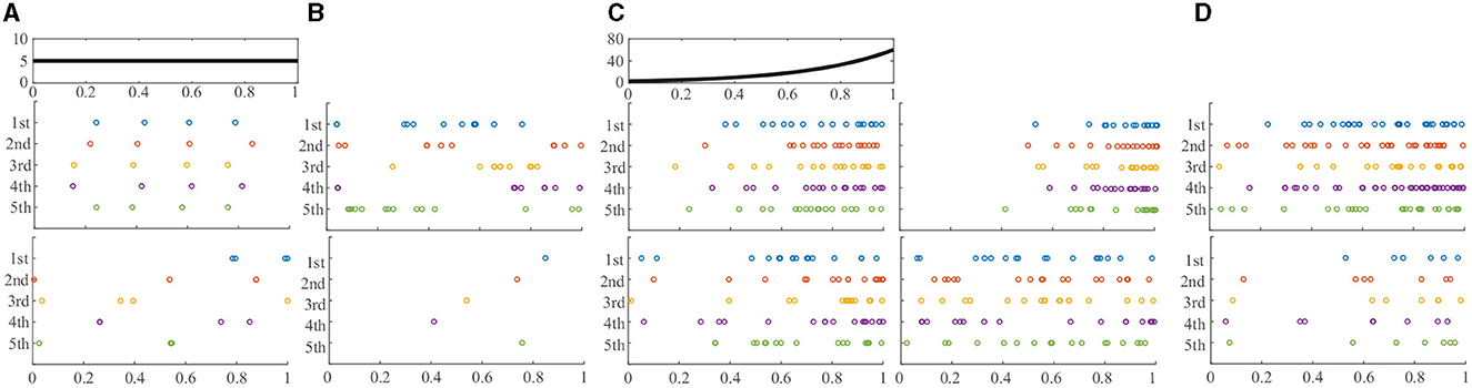
Figure 1. Comparisons of proposed and likelihoods in the ranking of Poisson process. (A) HPP K=4. (B) HPP across K. (C) IPP K=12. (D) IPP across K.

Based on Equation (6), we display the outliers (observations with 5 lowest modified likelihood values) in the first row of Figure 1B. These spike trains clearly do not exhibit a homogeneous pattern. In contrast, we display spike trains with 5 lowest classical likelihoods in the second row. These trains all have only 1 spike. These single-spike trains properly address the outlier type on the number of events, whereas they cannot capture the outliers with respect to the distribution of events.

We then generate 5,000 inhomogeneous Poisson process realizations on [0, 1] from the intensity function λ(t) = 3e^3t (exponentially increasing from 0 to 1), and the result for the cardinality being 12 is shown in Figure 1C. There are also 3 rows in this panel: the first row shows the intensity function, and the second row shows observations with the top five new likelihoods (left) in Equation (8) and classical likelihoods (right), respectively. We can see that the top spike trains using the new likelihood better represent intensity function than those using the classical likelihood. The third row in the panel shows observations with the bottom 5 new likelihoods (left) and classical likelihoods (right), respectively. In this case, both outlier groups exhibit different patterns from the intensity function.

We finally show the result across different cardinalities in the same inhomogeneous Poisson process realizations. In Figure 1D, we find the spike trains with top (upper row) and bottom (lower row) 5 modified likelihood estimations using Equation (9). We can also see that the typical spike trains (with high likelihoods) well capture the variability in intensity function, and the outliers (with low likelihoods) clearly exhibit discrepancy from the intensity.

3 Experimental results

In this section, we demonstrate the proposed new likelihood in a real experimental recording in the motor cortex, previously used in [11]. Spiking activity was recorded using a microelectrode array in the arm area of the primary motor cortex in a Macaque monkey. The monkey was trained to move a cursor to targets via contralateral arm movements in the horizontal plane by conducting a Squared-Path task. That is, in each trial, the monkey can start in any of the four corners and move in a counterclockwise direction to finish a square-shaped movement.

In each starting corner, the monkey conducted 60 trials of movement, and we have 240 trials in total in 4 different classes. 10 example spike trains of 2 typical cells in each starting point are shown in Figure 2 (left column). We take 20 trials in each class as the training data. The intensity in each class of each cell can be estimated via conventional kernel methods, and the result is shown in Figure 2B (middle column). For evaluating classification performance, we used the other 40 spike trains in each class as test data. The classification accuracy using the conventional likelihood method was 0.856 for Cell 1 and 0.831 for Cell 2. Using our new likelihood method, we achieved classification accuracies of 0.806 for both Cell 1 and Cell 2, comparable to those of the conventional likelihood. However, we employ the normalized rank-based likelihood. We find one outlier spike in Classes 1 and 4 for Cell 1 and one outlier spike in Class 4 for Cell 2, as depicted in Figure 2C (right column). After removing these outliers, we conducted the classification again and found the accuracies increased to 0.816 (Cell 1) and 0.811 (Cell 2), respectively. The findings demonstrate that our newly proposed likelihood method is effective in removing outliers, leading to an improvement in classification results when these outlier observations are excluded. Such outlier detection analysis cannot be accomplished under classical point process frameworks.

Figure 2

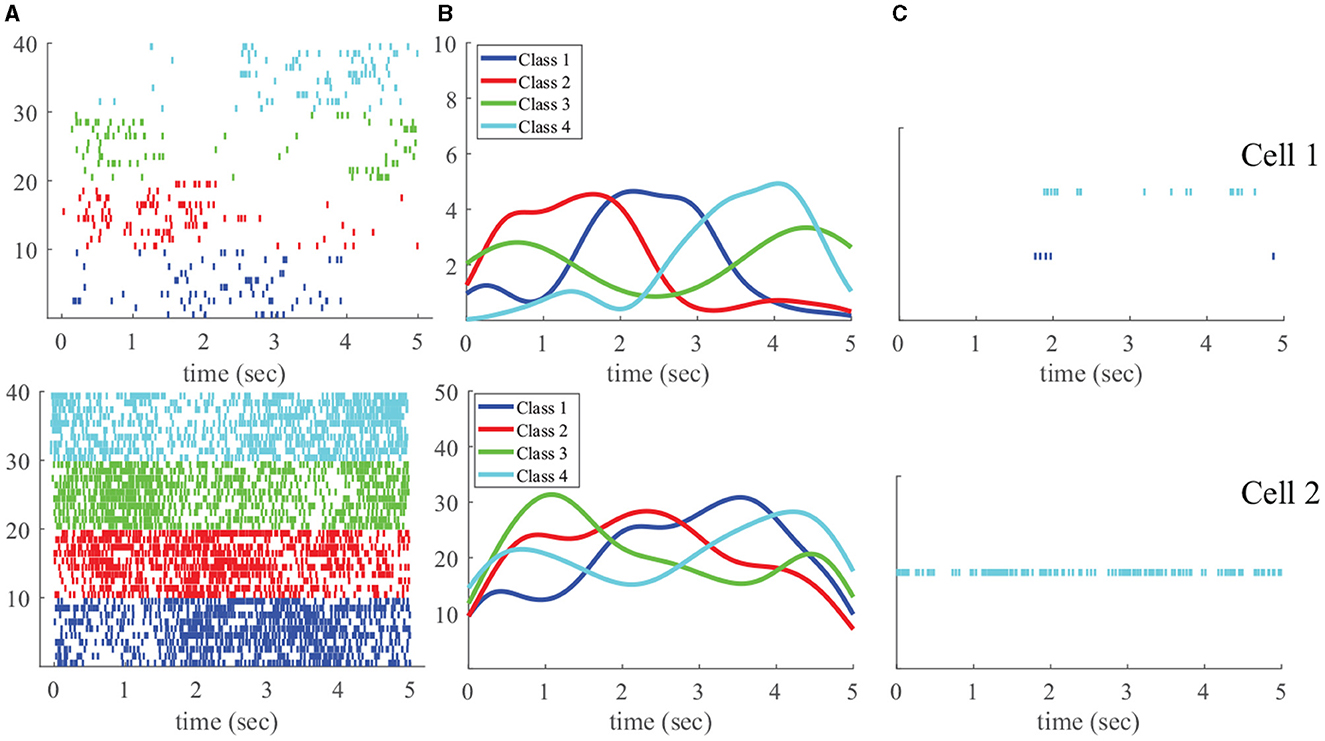
Figure 2. Real experimental data, where the top panels are for Cell 1, and the bottom ones are for Cell 2. (A) 10 example spike trains generated from each type of arm movement, with four distinct colors (blue, red, green, and cyan) representing four types of arm movements and associated spiking activities. Each thin vertical line indicates the time of a spike, and one row is for one trail; (B) Estimated intensity function; (C) Identified outliers using the proposed likelihood.

4 Discussion and future work

We have proposed a new rank-based likelihood that successfully indicates the centrality for observed spike trains for a given cardinality. Furthermore, we extend this rank-based likelihood to incorporate the cardinality and distribution of spikes to identify outliers. We have demonstrated the effectiveness of the new framework using simulations and real spike trains under the Poisson process assumption. In the future, we will extend this framework to more practical history-dependent point processes, such as a Hawks process. We will also explore the new method to conduct more useful applications, such as clustering and robust visualizations.

Data availability statement

The data analyzed in this study is subject to the following licenses/restrictions: the dataset is available upon request. Requests to access these datasets should be directed to WW, wwu@fsu.edu.

Author contributions

YM: Writing – original draft, Writing – review & editing. WW: Writing – original draft, Writing review & editing.

Funding

The author(s) declare that no financial support was received for the research, authorship, and/or publication of this article.

Conflict of interest

The authors declare that the research was conducted in the absence of any commercial or financial relationships that could be construed as a potential conflict of interest.

Publisher's note

All claims expressed in this article are solely those of the authors and do not necessarily represent those of their affiliated organizations, or those of the publisher, the editors and the reviewers. Any product that may be evaluated in this article, or claim that may be made by its manufacturer, is not guaranteed or endorsed by the publisher.

References

1. Perkel DH, Gerstein GL, Moore GP. Neuronal spike trains and stochastic point processes: II. simultaneous spike trains. Biophys J. (1967) 7:419–40. doi: 10.1016/S0006-3495(67)86597-4

PubMed Abstract | Crossref Full Text | Google Scholar

2. Richmond BJ, Optican LM, Spitzer H. Temporal encoding of two-dimensional patterns by single units in primate primary visual cortex. I Stimulus-response relations. J Neurophysiol. (1990) 64:351–69. doi: 10.1152/jn.1990.64.2.351

PubMed Abstract | Crossref Full Text | Google Scholar

3. Brown EN, Barbieri R, Ventura V, Kass RE, Frank LM. The time-rescaling theorem and its application to neural spike train data analysis. Neural Comput. (2002) 14:325–46. doi: 10.1162/08997660252741149

PubMed Abstract | Crossref Full Text | Google Scholar

4. Eden UT, Frank LM, Barbieri R, Solo V, Brown EN. Dynamic analysis of neural encoding by point process adaptive filtering. Neural Comput. (2004) 16:971–98. doi: 10.1162/089976604773135069

PubMed Abstract | Crossref Full Text | Google Scholar

5. Liu S, Wu W. Generalized mahalanobis depth in point process and its application in neural coding. Ann Appl Statist. (2017) 2017:992–1010. doi: 10.1214/17-AOAS1030

Crossref Full Text | Google Scholar

6. Qi K, Yang C, Wu W. Dirichlet depth for point process. Electron J Stat. (2021) 15:3574–610. doi: 10.1214/21-EJS1867

Crossref Full Text | Google Scholar

7. Xu Z, Wang C, Wu W. A unified framework on defining depth for point process using function smoothing. Comput Statist Data Analy. (2022) 175:107545. doi: 10.1016/j.csda.2022.107545

Crossref Full Text | Google Scholar

8. Aitchison J, Barceló-Vidal C, Martín-Fernández JA, Pawlowsky-Glahn V. Logratio analysis and compositional distance. Mathemat Geol. (2000) 32:271–5. doi: 10.1023/A:1007529726302

Crossref Full Text | Google Scholar

9. Zhou X, Ma Y, Wu W. Statistical depth for point process via the isometric log-ratio transformation. Comput Statist Data Analy. (2023) 187:107813. doi: 10.1016/j.csda.2023.107813

Crossref Full Text | Google Scholar

10. Egozcue JJ, Pawlowsky-Glahn V, Mateu-Figueras G, Barcelo-Vidal C. Isometric logratio transformations for compositional data analysis. Math Geol. (2003) 35:279–300. doi: 10.1023/A:1023818214614

Crossref Full Text | Google Scholar

11. Wu W, Srivastava A. An information-geometric framework for statistical inferences in the neural spike train space. J Comput Neurosci. (2013) 31:725–48. doi: 10.1007/s10827-011-0336-x

PubMed Abstract | Crossref Full Text | Google Scholar