Khalouta transform and applications to Caputo-fractional differential equations

1 Introduction

Fractional calculus extends the traditional calculus operation of differentiation and integral to non- integer orders. Although the concept finds its roots in the works of Euler, Laplace and Fourier in the 18th and 19th centuries, it has gained significant attention in recent years for its applications in diverse scientific and engineering fields. Solving fractional differential can be more challenging than solving traditional differential equations, and various numerical and analytical method [1–5] have been developed for this purpose. An integral transform is an operation that takes a function and maps it to another function through integration. It is often used to simplify and solve complex problems in various fields. The basic idea behind an integral transform is to express a function in terms of a different set of functions, making it easier to analyze and manipulate. One of the most well-known integral transforms is the Laplace transform [6, 7], which is widely used in control theory and signal processing. Another common integral transform is the Fourier transform, used in fields like signal analysis and image processing. These transforms have applications in solving differential equations, analyzing signals, and studying the frequency components of functions. Now days many integral transforms can be used to convert differential equations into algebraic equations, making them easier to solve such as Sumudu transform method, Natural transform method, Kamal transform method, Mohand transform method, Aboodh transform method, Shehu transform method [4], and Complex integral transform method etc. [8–32]. Integral transform are employed to solve partial differential equations governing heat transfer and fluid flow problems in engineering, such as in solving the heat conduction equation. The Fourier and wavelet transforms are used in image processing to analyze and enhance images, as well as to extract features and perform image compression [33–40]. The Khalouta integral transform is employed in this article to drive explanatory solutions for fractional differential equations utilizing both the both the Riemann-Liouville integral and caputo fractional derivative. The approach aims to provide a comprehensive understanding of the solutions within the context of these specific fractional calculus operators. Khalouta transform method for Atangana-Baleanu or other derivatives can also be adapted since Sumudu transform, Shehu transform and various other transforms exists for these derivatives and relationship of Khalouta transform exists with all these transforms. Applying Khalouta transform methods to highly nonlinear fractional differential equations can pose several challenges like analytical solutions complexity, convergence issues and others. Khalouta transform rely on the convergence of series or integrals. For highly nonlinear problems, convergence may be slow.

2 Pre-requisites

We present few fundamental definition and properties related to the fractional calculus. These definitions and properties form the basis for understanding and applying fractional calculus in various scientific and engineering disciplines. For detailed explanations, please refer to the cited sources [41, 42].

Definition 1 The Riemann Liouville fractional integral operator ${I_0}^{\beta }$ of order β for a function f:(0, ∞) → R for all β ∈ R⁺ is defined as,

$\begin{array}{ll}{I}_0{}^{\beta }f\left(u\right)=\frac{1}{\Gamma \left(\beta \right)}{\displaystyle {\int }_0^u{\left(u-\upsilon \right)}^{\beta -1}f(\upsilon )d\upsilon },& (1)\end{array}$

$=\frac{1}{\Gamma (\beta )}{u}^{\beta -1}*f(u),\beta >0,u>0,$

$I^{0}f(u)=f(u)$

Where Γ(.) is the widely known pseudo gamma function. It is an abstraction of factorial function,

$\begin{array}{ll}\Gamma p={\displaystyle {\int }_0^{\infty }{u}^{p-1}}{e}^{-u}dup\in c& (2)\end{array}$

Definition 2 The Riemann-Liouville fractional derivative operator ${}^R{D_u}^{\beta }$ of order β for a function f:(0, ∞) → R for all β ∈ R⁺ is defined as,

$\begin{array}{ll}{}^R{D}_u{}^{\beta }f(u)=D_u{}^n{I}^n{}^{-\beta }f(u)=\frac{d^n}{d{u}^n}{I}^n{}^{-\beta }f(u)& (3)\end{array}$

$\begin{array}{ll}=\frac{1}{\Gamma n-\beta }\frac{d^n}{d{u}^n}{\displaystyle {\int }_0^t{(u-\upsilon )}^{n-\beta -1}}f(\upsilon )d\upsilon ,u>0.& (4)\end{array}$

where n − 1 < β ≤ n  n ∈ N.

Definition 3 The Caputo fractional derivative of function f:(0, ∞) → R for all β ∈ R⁺ is defined as,

$\begin{array}{ll}\begin{array}{l}{}^c{D}_u{}^{\beta }f\left(u\right)=I^{n-\beta }{D}_u{}^{n}f\left(u\right)\hfill \\ =\frac{1}{\Gamma n-\beta }{\displaystyle {\int }_0^u{\left(u-\upsilon \right)}^{n-\beta -1}}{f}^n\left(\upsilon \right)d\upsilon ,u>0.\hfill \\ =\frac{{\partial }^n}{\partial u^n}f\left(u\right)=f^n(u).\hfill \end{array}& (5)\end{array}$

where n − 1 < β ≤ n   n ∈ N.

Definition 4 The Mittag-Leffler function is abstraction of exponential function E_β (k) which is defined as,

$\begin{array}{ll}{E}_{\delta }(k)={\displaystyle \sum _{r=0}^{\infty }}\frac{k^r}{\Gamma (\delta r+1)}& (6)\end{array}$

$\begin{array}{ll}{E}_{\delta ,\gamma }(k)={\displaystyle \sum _{r=0}^{\infty }}\frac{k^r}{\Gamma (\delta r+\gamma )}& (7)\end{array}$

here δ, γ ∈ R⁺and k ∈ c An abstraction of Mittag-Leffler function of is introduced by Prabhaker as given [43, 44]:

$\begin{array}{ll}{E}_{\delta ,\gamma }^{\epsilon }(k)={\displaystyle \sum _{r=0}^{\infty }}\frac{{(\epsilon )}_r}{\Gamma (\delta n+\gamma )}\frac{k^r}{r!}& (8)\end{array}$

here δ, γ, ε ∈ R⁺and k ∈ c

3 Khalouta transform

The function f:u ∈ [0, ∞[→ R of exponential order β > 0, then Khalouta transform, over the set of function is defined as [45]

$\varsigma =\left\{f(u):\exists K,\beta >0,\left|f(u)\right|<K\exp (\beta u),forallu\in [0,\infty [\right\},$

by the following integral

$\begin{array}{ll}Kh\left[f(u)\right]=k(s,\lambda ,\eta )=s{\displaystyle {\int }_0^{\infty }\exp (-su)f(\lambda \eta u)du.}& (9)\end{array}$

We can also define it as,

$Kh\left[f(u)\right]=k(s,\lambda ,\eta )=\frac{s}{\lambda \eta }{\displaystyle {\int }_0^{\infty }\exp \left(-\frac{su}{\lambda \eta }\right)}f(u)du$

or

$\begin{array}{ll}=\underset{\varphi \to \infty }{\lim }\frac{s}{\lambda \eta }{\displaystyle {\int }_0^{\varphi }\exp \left(-\frac{su}{\lambda \eta }\right)}f(u)du,& (10)\end{array}$

where s, λ, η > 0 are the Khalouta transform variables. β is a real number and the integral is taken along the limit u = ϕ. Equations (1–10) give the basic details of fractional operators and of Khalouta transform.

Since the Khalouta transform is very recently discovered so there might be some general queries about the efficiency and reliability of the transform but one can trust this transform as it has fair connections with other established transforms as well. Extending the Khalouta transform method to handle systems of fractional differential equations (FDEs) for improved efficiency and accuracy involves several considerations. Efficiency and accuracy depend on the specific characteristics of the system and the problem at hand. Khalouta transform possesses certain mathematical properties that make it suitable for solving problems related to Caputo fractional derivatives like, linearity, exponential behavior, derivatives property, initial value problem and semi group property. It can also be used to derive approximate solutions for fractional differential equations when exact solutions are challenging to obtain. Dealing with fractional orders involves performing computations related to fractional calculus. These computations can be more complex and computationally intensive than traditional integer-order calculus. Efficient algorithms and numerical methods may be needed. Fractional calculus problems may benefit from adaptive algorithms, such as adaptive time-stepping methods. These algorithms adjust the step size dynamically, which can impact the overall computation requirements. It's a complex area with challenges, and not all deep learning frameworks readily support fractional derivatives. we may need specialized tools or libraries designed for fractional calculus to address such multi-dimensional problem.

Khalouta transform methods can be applied to multidimensional problems involving partial derivatives with fractional orders in some scientific and engineering fields. Here are few examples: fractional heat equations, fractional wave equations and fractional diffusion equation. There are many examples from science and engineering where Khalouta transform has been successfully applied to solve real-world problems involving fractional calculus [1, 2]. The convergence properties of the transform method in solving fractional differential equations depend on the nature of the given problem. Generally, Khalouta transforms, can exhibit good convergence for well-behaved functions and problems with appropriate initial or boundary conditions. The convergence may be influenced by the smoothness of the solution, the decay properties of the involved functions, In some cases, careful consideration of the choice of fractional derivative definition (e.g., Caputo or Riemann-Liouville) is crucial for convergence analysis. This transform can also be extended to handle fractional integro differential equations like the first order volterra integro- differential equation with the initial condition and the second order volterra differential equations with the initial condition. When dealing with singularities or irregularities in fractional differential equations, specialized numerical techniques like the Caputo or Riemann-Liouville fractional differ-integration methods can be employed. These methods are designed to handle fractional calculus operations and may provide better performance in capturing the behavior of systems with singularities. Additionally, techniques such as fractional Adams-Bashforth or Adams-Moulton methods can be useful for solving fractional differential equations numerically. This transform may not be directly applicable to problems with variable order derivatives. These methods are most effective for problems with constant order derivatives. For variable order derivatives, you might need to explore specialized techniques like fractional calculus or other advanced mathematical tools, depending on the specific characteristics of our problem.

This transform method, often used for solving fractional differential equations (FDEs). The theoretical underpinning involves extending classical calculus to include fractional derivatives and integrals, allowing the analysis of systems with non-integer order derivatives. Mathematically, fractional derivatives are defined through integral operators, such as the Riemann-Liouville or Caputo operators. Transforming FDEs into the frequency or Laplace domain simplifies the equations, making them amenable to solution using standard techniques. This approach leverages the well-established properties of Khalouta transforms, enabling the application of existing mathematical tools to fractional calculus. There are some basic properties where Khalouta transform method fails to provide accurate solution like sudden changes or discontinuities in a function can lead to inaccuracies in transform solutions, Khalouta transforms may not converge for certain functions, leading to divergent or nonsensical results and incorrect or poorly defined boundary conditions can affect the accuracy of transform. Khalouta transform method can be generalized to address mixed fractional differential equations involving both Caputo and Riemann-Liouville fractional derivatives for future point of view. Till now no such study has been conducted. The choice of initial conditions and boundary conditions significantly influences the applicability and success of Khalouta transform method in solving fractional differential equations. Selecting appropriate conditions ensures the compatibility of the method with the problem at hand, enhancing convergence and accuracy. Incorrect choices may lead to divergence or inaccurate solutions, emphasizing the importance of a careful match between the problem's characteristics and the chosen conditions for a successful application of transform methods. Till now, there is no practical guidelines or best practices for researchers and practitioners when applying the Khalouta transform method to complex problems in fractional calculus. Integrating machine learning and AI techniques with the transform method holds potential for enhancing solutions to challenging fractional calculus problems. These technologies can improve accuracy, efficiency, and adaptability in handling complex mathematical operations, offering innovative approaches to problem-solving in this domain. If we clearly compare this transform with other transforms then we can say that this is another tool we have got to address the scientific and technical problems. The efficiency of the Khalouta transform method compare to other numerical methods commonly used in fractional calculus, such as the finite difference method or the Laplace transform method is not done till now but it can be a new vertical for the future studies as well. Since this is the newly introduced transform so till now not much work has been done with this so the classes of problems where Khalouta transform outperforms other existing techniques, is not defined till now. This was the some basic and important information about the Khalouta transform which can help the researchers to think in some new vertical of the solutions.

3.1 Khalouta—Shehu duality

Let k(s, λ, η) be the Khalouta transform of the function f(u) ∈ ς. If we take η = 1 then equation become,

$\begin{array}{ll}k(s,\lambda ,1)=\frac{s}{\lambda }{\displaystyle \underset{0}{\overset{\infty }{\int }}}exp(\frac{-su}{\lambda })f(u)du=\frac{s}{\lambda }Sh(s,\lambda )& (11)\end{array}$

where Sh(s, λ) denotes the Shehu transform of the function f(u) ∈ ς.

Corollary Shehu transform of Mittag–Leffler function [46],

$E_{\delta ,\gamma }(k)=,{\displaystyle \sum _{r=0}^{\infty }}\frac{k^r}{\Gamma (\delta r+\gamma )}\delta ,\gamma \in C,\text{ Re}(\delta ),\text{Re}(\gamma )>0$

exists and is given as

$\begin{array}{ll}Sh(u^{\gamma -1}{E}_{\delta ,\gamma }^{\epsilon }(w{u}^{\delta }))={\left(\frac{\lambda }{s}\right)}^{\gamma }{\left(1-w{\left(\frac{\lambda }{s}\right)}^{\delta }\right)}^{-\epsilon }& (12)\end{array}$

if we take ω = −1 and ε = −1 Equation (12) becomes

$Sh(u^{\gamma -1}{E}_{\delta ,\gamma }(-u^{\delta }))={\left(\frac{\lambda }{s}\right)}^{\gamma }{\left(1+{\left(\frac{\lambda }{s}\right)}^{\delta }\right)}^{-1}$

or,

$Sh(E_{\delta }(-u^{\delta }))=\left(\frac{\lambda }{s}\right){\left(1+{\left(\frac{\lambda }{s}\right)}^{\delta }\right)}^{-1}$

Using relation (Equation 11), we can find Khalouta transform of Mittag- Leffler function as

$\begin{array}{ll}Kh\left[E_{\delta }(-u^{\delta })\right]={\left(1+{\left(\frac{\lambda \eta }{s}\right)}^{\delta }\right)}^{-1}& (13)\end{array}$

3.2 Some basic properties of Khalouta transform

Now we are going to discuss some properties of Khalouta transform.

a. Linear property of the Khalouta transform If λ and μ are non- zero arbitrary constants and f(u) and g(u) are functions defined over the set ς, then (λf(u) + μg(u)) ∈ ς, and (Equation 14)

$\begin{array}{ll}Kh\left[\lambda f(u)\pm \mu g(u)\right]=\lambda Kh\left[f(u)\right]\pm \mu Kh\left[g(u)\right].& (14)\end{array}$

b. Khalouta transform of derivatives of the functions Let f(u) be the function, then n^th derivative of the function is defined as fⁿ(u) ∈ ς with respect to u. For n = 1, 2, 3, …… and its Khalouta transform is specified,

$\begin{array}{ll}Kh\left[f^n(u)\right]=\frac{s^n}{{\lambda }^n{\eta }^n}k(s,\lambda ,\eta )-{\displaystyle \sum _{k=0}^{n-1}}{\left(\frac{s}{\lambda n}\right)}^{n-k}{f}^k(0).& (15)\end{array}$

Here we also define the Khalouta transform of n^th partial derivative. Let v = v(x, t) and $\frac{{\partial }^{n}v(x,t)}{\partial x^n}$ both defined in the set ς. And suppose k(x, s, λ, η,) be the Khalouta transform of v(x, t) and $\frac{{\partial }^{n}v(x,t)}{\partial x^n}$ is the n^th derivative of the function v(x, t) with respect to x. Then

$\begin{array}{ll}Kh\left[\frac{{\partial }^{n}v(x,t)}{\partial x^n}\right]=\frac{d^n}{d{x}^n}k(x,s,\lambda ,\eta )& (16)\end{array}$

where n = 1, 2, 3, …

c. Khalouta transform of the convolution of two functions Suppose k₁(s, λ, η)and k₂(s, λ, η) are the Khalouta transforms of f(u) and g(u), respectively, both defined in the set ς. Then the Khalouta transform of their convolution is given by (Equation 17),

$\begin{array}{ll}Kh\left[(f*g)u\right]=\frac{\lambda \eta }{s}{k}_1(s,\lambda ,\eta )k_2(s,\lambda ,\eta ),& (17)\end{array}$

where (f * g) is convolution of two functions defined as,

$(f*g)(u)={\displaystyle {\int }_0^{u}f(\tau )g(u-\tau )d\tau ={\displaystyle {\int }_0^{u}f(u-\tau )}}g(u)d\tau .$

d. Khalouta transform for some functions Below are the Khalouta transforms of some standard functions:

$Kh\left(\frac{u^{p-1}}{\Gamma p}\right)=\frac{{\lambda }^{p-1}{\eta }^{p-1}}{s^{p-1}}$

$Kh\left[sin\beta t\right]=\frac{\beta s\lambda \eta }{s^2+{\beta }^2{\lambda }^2{\eta }^2}.$

$Kh\left[sinh\beta t\right]=\frac{\beta s\lambda \eta }{s^2-{\beta }^2{\lambda }^2{\eta }^2}.$

$Kh\left[cos\beta t\right]=\frac{s^2}{s^2+{\beta }^2{\lambda }^2{\eta }^2}.$

$Kh\left[cosh\beta t\right]=\frac{s^2}{s^2-{\beta }^2{\lambda }^2{\eta }^2}.$

$Kh\left[e^{-at}\right]=\frac{s}{s+a\lambda \eta }$

e. Khalouta transform of some fractional derivatives

3.2.1 Theorem 1

Suppose that k(s, λ, η) be the Khalouta integral transform of the function f(u), which satisfy n ∈ Z⁺ and n − 1 < β ≤ n, then the Khalouta integral transform of the Riemann-Liouville fractional integral of f(u) of order β > 0, is

$\begin{array}{ll}Kh\left[{I_0}^{\beta }f(u)\right]=\left(\frac{{\lambda }^{\beta }{\eta }^{\beta }}{s^{\beta }}\right)k(s,\lambda ,\eta )& (18)\end{array}$

Proof For the function f(u) , the Riemann Liouville fractional integral ${I_0}^{\beta }$ can be expressed as the convolution by ${I_0}^{\beta }f(u)=\frac{1}{\Gamma \beta }{u}^{\beta -1}*f(u).$ Now, by applying the Khalouta transform of the convolution of two function (property c), we have

$\begin{array}{l}Kh\left[I_0{}^{\beta }f(u)\right]=Kh\left[\frac{1}{\Gamma \beta }{u}^{\beta -1}*f(u)\right]\\ =\frac{\lambda \eta }{s}Kh\left[\frac{u^{\beta -1}}{\Gamma \beta }\right]Kh\left[f\left(u\right)\right]\end{array}$

now using property (d) we get

$=\frac{\lambda \eta }{s}\left(\frac{{\lambda }^{\beta -1}{\eta }^{\beta -1}}{s^{\beta -1}}\right)k(s,\lambda ,\eta )$

or,

$={\left(\frac{\lambda \eta }{s}\right)}^{\beta }k(s,\lambda ,\eta )$

Hence Proved.

3.2.2 Theorem 2

Suppose that k(s, λ, η) be the Khalouta integral transform of the function f(u), which satisfy n ∈ Z⁺ and n − 1 < β ≤ n , then the Khalouta integral transform of the Riemann-Liouville fractional derivative of f(u) of order β > 0, is

$Kh\left[{}^R{D}_u{}^{\beta }f(u)\right]={\left(\frac{\lambda \eta }{s}\right)}^{-\beta }k(s,\lambda ,\eta )-{\displaystyle \sum _{k=0}^{n-1}{\left(\frac{s}{\lambda \eta }\right)}^k}{{[}^R{D}_u{}^{\beta -k}f(u)]}_{u=0}$

Proof Let us consider the function

$\begin{array}{ll}g(u)={I_0}^{n-\beta }f(u)& (19)\end{array}$

Now, applying Khalouta transform of Equation (19) and using Equation (18), we have

$\begin{array}{l}Kh\left[g(u)\right]=Kh[I_0{}^{n-\beta }f(u)]={\left(\frac{\lambda \eta }{s}\right)}^{n-\beta }k\left(s,\lambda ,\eta \right)\\ Kh\left[g(u)\right]=G\left(s,\lambda ,\eta \right)={\left(\frac{\lambda \eta }{s}\right)}^{n-\beta }k\left(s,\lambda ,\eta \right)& (20)\end{array}$

then, from the definition of Riemann-Liouville fractional derivative (2), we have

$\begin{array}{ll}\begin{array}{c}{}^R{D}_u{}^{\beta }f(u)=D_u{}^n{I}_0{}^{n-\beta }f(u)=\frac{d^n}{d{u}^n}{I}_0{}^{n-\beta }f(u)\\ =\frac{d^n}{d{u}^n}g(u)\\ {}^R{D}_u{}^{\beta }f(u)=g^n(u)\end{array}& (21)\end{array}$

Applying the Khalouta transform on Equation (21) both the sides,

$Kh\left[{}^R{D}_u{}^{\beta }f(u)\right]=Kh\left[g^n(u)\right]$

Now we use property (b), we have

$\begin{array}{l}Kh\left[{}^R{D}_u{}^{\beta }f(u)\right]=\left(\frac{s^n}{{\lambda }^n{\eta }^n}\right)G(s,\lambda ,\eta )-{\displaystyle \sum _{k=0}^{n-1}{\left(\frac{s}{\lambda \eta }\right)}^{n-k}}[g^k(u){]}_{u=0}\\ Kh\left[{}^R{D}_u{}^{\beta }f(u)\right]=\left(\frac{s^n}{{\lambda }^n{\eta }^n}\right)G(s,\lambda ,\eta )-{\displaystyle \sum _{k=0}^{n-1}{\left(\frac{s}{\lambda \eta }\right)}^k}[g^{n-k}(u){]}_{u=0}\end{array}$

this equation can also be written as

$\begin{array}{r}\hfill Kh\left[{}^R{D}_u{}^{\beta }f(u)\right]=\left(\frac{s^n}{{\lambda }^n{\eta }^n}\right)G(s,\lambda ,\eta )-{\displaystyle \sum _{k=0}^{n-1}{\left(\frac{s}{\lambda \eta }\right)}^k}\\ \hfill {[D_t{}^{n-k}{I}_0{}^{n-\beta }f(u)]}_{t=0}\end{array}$

Using Equation (20) and definition (2), we have

$\begin{array}{r}\hfill Kh\left[{}^R{D}_u{}^{\beta }f(u)\right]=\left(\frac{s^n}{{\lambda }^n{\eta }^n}\right)\\ \hfill {\left(\frac{\lambda \eta }{s}\right)}^{n-\beta }k(s,\lambda ,\eta )-{\displaystyle \sum _{k=0}^{n-1}{\left(\frac{s}{\lambda \eta }\right)}^k}{{[}^R{D}_u{}^{\beta -k}f(u)]}_{u=0}\\ \hfill Kh\left[{}^R{D}_u{}^{\beta }f(u)\right]={\left(\frac{\lambda \eta }{s}\right)}^{-\beta }k(s,\lambda ,\eta )-{\displaystyle \sum _{k=0}^{n-1}{\left(\frac{s}{\lambda \eta }\right)}^k}\\ \hfill {{[}^R{D}_u{}^{\beta -k}f(u)]}_{u=0}.\end{array}$

Hence Proved.

3.2.3 Theorem 3

Suppose that k(s, λ, η) be the Khalouta integral transform of the function f(u), which satisfy n ∈ Z⁺ and n − 1 < β ≤ n , then the Khalouta integral transform of Caputo fractional derivative of f(u) of order β > 0, is

$\begin{array}{ll}Kh{[}^c{{{\displaystyle D}}_u}^{\beta }f(u)]={\left(\frac{\lambda \eta }{s}\right)}^{-\beta }k(s,\lambda ,\eta )-{\displaystyle \sum _{k=0}^{n-1}{\left(\frac{\lambda \eta }{s}\right)}^{-\beta +k}}{f}^k(0)& (22)\end{array}$

Proof By definition (3) of the Caputo fractional derivative of function, we have,

$\begin{array}{ll}\begin{array}{c}{}^c{{{\displaystyle D}}_u}^{\beta }f(u)=\frac{1}{\Gamma n-\beta }{\displaystyle {\int }_0^u{(u-\upsilon )}^{n-\beta -1}}{f}^n(\upsilon )d\upsilon \\ =\frac{1}{\Gamma n-\beta }{\displaystyle {\int }_0^u{(u-\upsilon )}^{n-\beta -1}}g(\upsilon )d\upsilon \\ {}^c{{{\displaystyle D}}_u}^{\beta }f(u)=I_0{}^{n-\beta }g(u)\end{array}& (23)\end{array}$

by applying the Khalouta transform on both sides of Equation (23) and using theorem 1, as a result,

$\begin{array}{ll}Kh\left[{}^c{D}_u{}^{\beta }f(u)\right]=Kh\left[I_0{}^{n-\beta }g(u)\right]={\left(\frac{\lambda \eta }{s}\right)}^{n-\beta }G(s,\lambda ,\eta )& (24)\end{array}$

where G(s, λ, η) is the Khalouta integral transform of the function g(u). Now, applying Khalouta transform and using the property (b), we obtain

$\begin{array}{c}Kh[g(u)]=Kh[f^n(u)]\\ G(s,\lambda ,\eta )=Kh[f^n(u)]=\frac{s^n}{{\lambda }^n{\eta }^n}k(s,\lambda ,\eta )-{\displaystyle \sum _{k=0}^{n-1}{\left(\frac{s}{\lambda n}\right)}^{n-k}}{f}^k(0)]\end{array}$

Therefore, the Equation (24) becomes

$\begin{array}{ll}\begin{array}{c}Kh{[}^c{D}_u{}^{\beta }f(u)]={\left(\frac{\lambda \eta }{s}\right)}^{n-\beta }\\ \left[\left(\frac{s^n}{{\lambda }^n{\eta }^n}\right)k\left(s,\lambda ,\eta \right)-{\displaystyle \sum _{k=0}^{n-1}{\left(\frac{s}{\lambda \eta }\right)}^{n-k}{f}^k\left(0\right)}\right]\\ Kh{[}^c{D}_u{}^{\beta }f(u)]={\left(\frac{\lambda \eta }{s}\right)}^{-\beta }k(s,\lambda ,\eta )-{\displaystyle \sum _{k=0}^{n-1}{\left(\frac{\lambda \eta }{s}\right)}^{-\beta +k}}{f}^k(0).\end{array}& (25)\end{array}$

where n − 1 < β ≤ n

which gives Equation (22), hence from Equation (25), we get our result.

This article is divided into five parts. Part one is consisting of origination of the article. Section 2 is dealing with pre-requisites related to the paper. Khalouta transform and some properties are discussed in segment 3 while Section 4 is having application part. Paper is concluded in Section 5. List of references is attached at the end to acknowledge the researchers and mathematicians.

4 Applications

In this segment, we are going to discuss some particular applications of Khalouta transform in solving the fractional differential equations. Using fractional order, here we take a linear ordinary differential equation [46].

$\begin{array}{ll}{}^c{D}_u{}^{\beta }y(u)={\displaystyle \sum _{j=1}^n{b}_j}{y}^{\left(j\right)}(u)+g(u)& (26)\end{array}$

with initial conditions

$\begin{array}{ll}\begin{array}{l}{y}^{(j)}(0)=a_j,j=0,\mathrm{\dots }n-1,\hfill \\ a_j,b_j\in R,g(u)\in A\hfill \end{array}& (27)\end{array}$

we take Khalouta transform of Equation (26), and we secure

$Kh\left[{}^c{D}_u{}^{\beta }y(u)\right]=Kh\left[{\displaystyle \sum _{j=1}^n{b}_j}{y}^{\left(j\right)}(u)+g(u)\right]$

now by the linearity property of Khalouta transform, we have

$\begin{array}{l}Kh\left[{}^c{D}_u{}^{\beta }y(u)\right]={\displaystyle \sum _{j=0}^n{b}_j}Kh\left(y^{(j)}(u)\right)+Kh\left(g(u)\right)\hfill \\ Kh\left[{}^c{D}_u{}^{\beta }y(u)\right]=b_{0}y(u)+{\displaystyle \sum _{j=1}^n{b}_{j}Kh\left(y^{(j)}(u)\right)+Kh\left(g(u)\right)}\hfill \end{array}$

Using theorem 3 and property (b), we obtain

$\begin{array}{l}{\left(\frac{\lambda \eta }{s}\right)}^{-\beta }Y(s,\lambda ,\eta )-{\displaystyle \sum _{k=0}^{n-1}{\left(\frac{\lambda \eta }{s}\right)}^{-\beta +k}}{y}^k(0)=b_{0}Y(s,\lambda ,\eta )+{\displaystyle \sum _{j=1}^n{b}_j}+\hfill \\ \left[\frac{s^j}{{\lambda }^j{\eta }^j}Y(s,\lambda ,\eta )-{\displaystyle \sum _{k=0}^{j-1}{\left(\frac{s}{\lambda \eta }\right)}^{j-k}}{y}^k(0)\right]+Kh\left(g(u)\right)\hfill \\ +{\left(\frac{\lambda \eta }{s}\right)}^{-\beta }Y(s,\lambda ,\eta )-{\displaystyle \sum _{j=0}^n{b}_j}\frac{s^j}{{\lambda }^j{\eta }^j}Y(s,\lambda ,\eta )={\displaystyle \sum _{k=0}^{n-1}{a}_k{\left(\frac{\lambda \eta }{s}\right)}^{-\beta +k}}\hfill \\ -{\displaystyle \sum _{j=1}^n{b}_j}{\displaystyle \sum _{k=0}^{j-1}{a}_k}{\left(\frac{s}{\lambda \eta }\right)}^{j-k}+Kh(g(u))\hfill \end{array}$

or by using Equation (27), we have,

$\begin{array}{ll}\begin{array}{l}Y(s,\lambda ,\eta )={\left({\left(\frac{\lambda \eta }{s}\right)}^{-\beta }-{\displaystyle \sum _{j=0}^n{b}_j}\frac{s^j}{{\lambda }^j{\eta }^j}\right)}^{-1}\hfill \\ \times \left({{\displaystyle \sum _{k=0}^{n-1}{a}_k\left(\frac{\lambda \eta }{s}\right)}}^{-\beta +k}-{\displaystyle \sum _{j=1}^n{b}_j}{\displaystyle \sum _{k=0}^{j-1}{a}_k}{\left(\frac{s}{\lambda \eta }\right)}^{j-k}+Kh(g(u))\right)\hfill \end{array}& (28)\end{array}$

By using inverse Khalouta transform on of Equation (28), and we secure result of Equation (26) as,

$\begin{array}{ll}\begin{array}{l}y(u)=K{h}^{-1}[{\left({\left(\frac{\lambda \eta }{s}\right)}^{-\beta }-{\displaystyle \sum _{j=0}^n{b}_j}\frac{s^j}{{\lambda }^j{\eta }^j}\right)}^{-1}\hfill \\ \times \left({{\displaystyle \sum _{k=0}^{n-1}{a}_k\left(\frac{\lambda \eta }{s}\right)}}^{-\beta +k}-{\displaystyle \sum _{j=1}^n{b}_j}{\displaystyle \sum _{k=0}^{j-1}{a}_k}{\left(\frac{s}{\lambda \eta }\right)}^{j-k}+Kh(g(u))\right)]\hfill \end{array}& (29)\end{array}$

4.1 Example 1

When n = 1, b₀ = −1, b₁ = g(u) = 0 we secure [47],

$\begin{array}{ll}{}^c{D}_u{}^{\beta }y(u)+y(u)=0,0<\beta \le 1,u>0& (30)\end{array}$

with initial condition y(0) = 1

Solution Substituting n, b₀, b₁, and g in Equation (29), we get

$y(u)=K{h}^{-1}\left[{\left({\left(\frac{\lambda \eta }{s}\right)}^{-\beta }-{\displaystyle \sum _{j=0}^1}{b}_j\frac{s^j}{{\lambda }^j{\eta }^j}\right)}^{-1}{\left(\frac{\lambda \eta }{s}\right)}^{-\beta }\right]$

or,

$y(u)=K{h}^{-1}\left[{\left(1-(-1){\left(\frac{\lambda \eta }{s}\right)}^{\beta }\right)}^{-1}\right]$

or

$y(u)=K{h}^{-1}{\left(1+{\left(\frac{\lambda \eta }{s}\right)}^{\beta }\right)}^{-1}$

Thus, by Khalouta transform of Mittag-Leffler function of Equation (13), we have

$Y(s,\lambda ,\eta )=Kh(E_{\beta }(-u^{\beta }))$

We get absolute result of Equation (30) as (Figure 1),

$y(u)=E_{\beta }(-u^{\beta })$

Figure 1

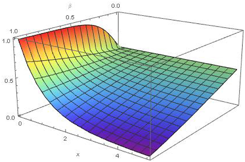
Figure 1. Graph of solution obtained in example 1.

4.2 Example 2

Let we take homogeneous ordinary differential equation with fractional order [48].

$\begin{array}{ll}{}^c{D}_u{}^{\frac{1}{2}}y(u)+y(u)=u^2+\frac{\Gamma \left(3\right)}{\Gamma \left(\frac{5}{2}\right)}{u}^{\frac{3}{2}},u>0& (31)\end{array}$

with initial condition y(0) = 0.

Solution Now we have to find absolute result of Equation (31), so we take Equation (29), for n = 1, b₀ = −1, b₁ = 0 and $g(u)=u^2+\frac{\Gamma (3)}{\Gamma (\frac{5}{2})}{u}^{\frac{3}{2}}$, we get

$y(u)=K{h}^{-1}\left[{\left({\left(\frac{\lambda \eta }{s}\right)}^{-\frac{1}{2}}-(-1)\right)}^{-1}Kh\left(u^2+\frac{\Gamma (3)}{\Gamma \frac{5}{2}}{u}^{\frac{3}{2}}\right)\right]$

or,

$\begin{array}{l}y(u)=K{h}^{-1}\left[{\left({\left(\frac{\lambda \eta }{s}\right)}^{-\frac{1}{2}}-(-1)\right)}^{-1}\left(2{\left(\frac{\lambda \eta }{s}\right)}^2+\frac{\Gamma (3)}{\Gamma (\frac{5}{2})}{\left(\frac{\lambda \eta }{s}\right)}^{\frac{3}{2}}\Gamma \left(\frac{5}{2}\right)\right)\right]\end{array}$

or,

$y(u)=K{h}^{-1}\left[\left(2{\left(\frac{\lambda \eta }{s}\right)}^2\right)\left(\frac{\left({\left(\frac{\lambda \eta }{s}\right)}^{-\frac{1}{2}}+1\right)}{\left({\left(\frac{\lambda \eta }{s}\right)}^{-\frac{1}{2}}-(-1)\right)}\right)\right]$

or,

$y(u)=K{h}^{-1}\left(2{\left(\frac{\lambda \eta }{s}\right)}^2\right)$

or, finally we get (Figure 2)

$y(u)=u^2$

Figure 2

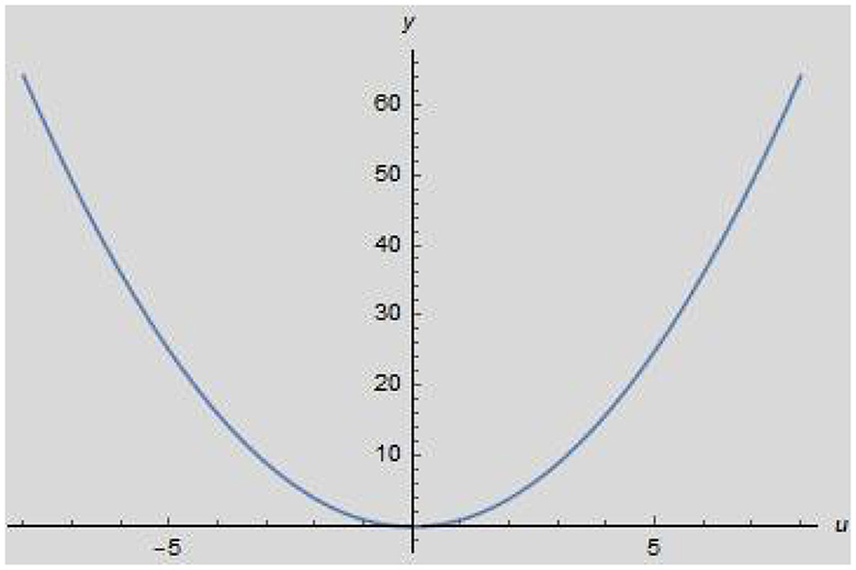
Figure 2. Graph of solution obtained in example 2.

4.3 Example 3

Consider the wave equation [49].

$\begin{array}{ll}\frac{{\partial }^{2}u(x,t)}{\partial t^2}-4\frac{{\partial }^{2}u(x,t)}{\partial x^2}=0& (32)\end{array}$

with initial conditions

$\begin{array}{ll}u(x,0)=sin\pi x,u_t(x,0)=0andx,t>0& (33)\end{array}$

Solution Taking the Khalouta transform of Equation (32) and using Equations (15, 16) of Property (b), we obtain

$\begin{array}{ll}\begin{array}{l}\text{}\frac{d^2}{d{t}^2}k\left(x,s,\lambda ,\eta \right)\hfill \\ -4\left[\frac{s^2}{{\lambda }^2{\eta }^2}k\left(x,s,\lambda ,\eta \right)-\frac{s^2}{{\lambda }^2{\eta }^2}u\left(x,0\right)-\frac{s}{\lambda \eta }{u}_t\left(x,0\right)\right]=0\hfill \end{array}& (34)\end{array}$

Using initial conditions (Equation 33) and simplifying the Equation (34), we obtain

$\frac{d^2}{d{t}^2}k(x,s,\lambda ,\eta )-4\frac{s^2}{{\lambda }^2{\eta }^2}k(x,s,\lambda ,\eta )+4\frac{s^2}{{\lambda }^2{\eta }^2}sin(\pi x)=0$

or,

$\begin{array}{ll}\frac{{\lambda }^2{\eta }^2}{4s^2}\frac{d^2}{d{t}^2}k(x,s,\lambda ,\eta )-k(x,s,\lambda ,\eta )=-sin(\pi x)& (35)\end{array}$

Which is linear ordinary differential equation with second order, so that the overall result of Equation (35) can be put down,

$k(x,s,\lambda ,\eta )=\frac{-sin(\pi x)}{\frac{{\lambda }^2{\eta }^2}{4s^2}{D}^2-1}=\frac{-sin(\pi x)}{\frac{{\lambda }^2{\eta }^2}{4s^2}(-{\pi }^2)-1}$

or,

$=\frac{s^2}{{\left(\frac{\pi }{2}\right)}^2{\lambda }^2{\eta }^2+s^2}sin(\pi x)$

by using the inverse Khalouta transform of above, the absolute result of Equation (32) (Figure 3) is

$u(x,t)=cos\frac{\pi }{2}t.sin(\pi x).$

Figure 3

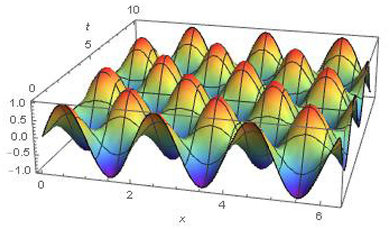
Figure 3. Graph of solution obtained in example 3.

4.4 Example 4

Let we take the homogeneous heat equation [49].

$\begin{array}{ll}4\frac{\partial u(x,t)}{\partial t}=\frac{{\partial }^{2}u(x,t)}{\partial x^2}& (36)\end{array}$

with initial condition

$\begin{array}{ll}u(x,0)=sin\frac{\pi }{2}x,x,t>0& (37)\end{array}$

Solution Applying the Khalouta transform on Equation (36), we have

$Kh\left[4\frac{\partial u(x,t)}{\partial t}\right]=Kh\left[\frac{{\partial }^{2}u(x,t)}{\partial x^2}\right]$

Using Equations (15, 16) of property (b), and we obtain,

$\begin{array}{ll}\frac{d^2}{d{x}^2}k(x,s,\lambda ,\eta )-4\left[\frac{s}{\lambda \eta }k(x,s,\lambda ,\eta )-\frac{s}{\lambda \eta }u(x,0)\right]=0& (38)\end{array}$

Using the initial conditions (Equation 37) and simplifying the Equation (38), we obtain

$\begin{array}{ll}\frac{d^2}{d{x}^2}k(x,s,\lambda ,\eta )-4\frac{s}{\lambda \eta }k(x,s,\lambda ,\eta )=-4\frac{s}{\lambda \eta }sin\frac{\pi }{2}x& (39)\end{array}$

which is linear ordinary differential equation with second order. The overall result of Equation (39) can be put down

$k(x,s,\lambda ,\eta )=\frac{-\frac{4s}{\lambda \eta }sin\frac{\pi }{2}x}{D^2-\frac{4s}{\lambda \eta }}=\frac{-\frac{4s}{\lambda \eta }sin\frac{\pi }{2}x}{-\frac{{\pi }^2}{4}-\frac{4s}{\lambda \eta }}$

or,

$k(x,s,\lambda ,\eta )=\frac{s}{\frac{{\pi }^2}{16}\lambda \eta +s}sin\frac{\pi }{2}x$

by using the inverse Khalouta transform of the above, the absolute result of Equation (36) (Figure 4) is reported by

$u(x,t)=e^{-\frac{{\pi }^2}{16}t}.sin\frac{\pi }{2}x$

Figure 4

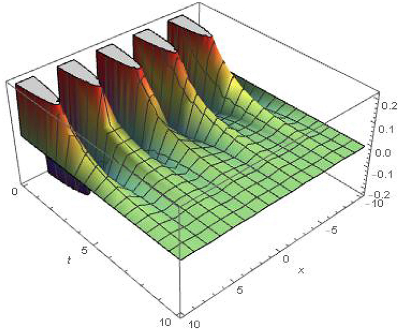
Figure 4. Graph of solution obtained in example 4.

5 Conclusion

The Khalouta transform method appears to be a valuable approach for addressing Riemann-Liouville fractional derivatives and integrals, as well as Caputo fractional derivatives. The successful application of this mehod in resolving examples suggests its efficacy and efficiency in obtaining exact solutions for fractional differential equations involving Caputo derivatives and partial derivatives. This could contribute to advancements in solving complex mathematical problems in the realm of fractional calculus.

Data availability statement

The original contributions presented in the study are included in the article/supplementary material, further inquiries can be directed to the corresponding author.

Author contributions

NK: Writing – original draft. AS: Writing – review & editing. MM: Writing – original draft. RS: Writing – review & editing. RD: Supervision, Validation, Writing – original draft.

Funding

The author(s) declare that no financial support was received for the research, authorship, and/or publication of this article.

Conflict of interest

The authors declare that the research was conducted in the absence of any commercial or financial relationships that could be construed as a potential conflict of interest.

Publisher's note

All claims expressed in this article are solely those of the authors and do not necessarily represent those of their affiliated organizations, or those of the publisher, the editors and the reviewers. Any product that may be evaluated in this article, or claim that may be made by its manufacturer, is not guaranteed or endorsed by the publisher.

References

1. Khalouta A, Kadem A. A new method to solve fractional differential equations: inverse fractional Shehu transform method. Appl Appl Math. (2019) 14:19. doi: 10.17512/jamcm.2020.3.04

Crossref Full Text | Google Scholar

2. Khalouta A. A new general integral transform for solving Caputo fractional-order differential equations. Int J Nonlinear Anal Appl. (2023) 14:67–78.

Google Scholar

3. Thange TG, Gade AR. On Aboodh transform for fractional differential operator. Malaya J Mathematik. (2020) 8:225–9. doi: 10.26637/MJM0801/0038

Crossref Full Text | Google Scholar

4. Maitama S, Zhao W. New integral transform: Shehu transform a generalization of Sumudu and Laplace transform for solving differential equations. arXiv [preprint]. (2019). doi: 10.48550/arXiv.1904.11370

Crossref Full Text | Google Scholar

5. Ahmadi SAP, Hosseinzadeh H, Cherati AY. A new integral transform for solving higher order linear ordinary Laguerre and Hermite differential equations. Int J Appl Comp Math. (2019) 5:1–7. doi: 10.1007/s40819-019-0712-1

Crossref Full Text | Google Scholar

6. Debnath L, Debnath L. Nonlinear Partial Differential Equations for Scientists and Engineers. Boston, MA: Birkhäuser (2005). p. 528–9.

Google Scholar

7. Patil D. Application of integral transform (Laplace and Shehu) in chemical sciences. Aayushi Int Interdiscip Res J. (2022). doi: 10.2139/ssrn.4006213

Crossref Full Text | Google Scholar

8. Rezapour S, Etemad S, Asamoah JKK, Ahmad H, Nonlaopon K. A mathematical approach for studying the fractal-fractional hybrid Mittag-Leffler model of malaria under some control factors. AIMS Math. (2023) 8:3120–62. doi: 10.3934/math.2023161

Crossref Full Text | Google Scholar

9. Alqahtani AM, Shukla A. Computational analysis of multi-layered Navier—Stokes system by Atangana—Baleanu derivative. Appl Math Sci Eng. (2024) 32:2290723. doi: 10.1080/27690911.2023.2290723

Crossref Full Text | Google Scholar

10. Dubey RS, Baleanu D, Mishra M, Goswami P. Solution of modified Bergman's minimal blood glucose insulin model using caputo-fabrizio fractional derivative. CMES. (2021) 128:1247–63. doi: 10.32604/cmes.2021.015224

Crossref Full Text | Google Scholar

11. Khan MA, Ullah S, Kumar S. A robust study on 2019-nCOV outbreaks through non-singular derivative. Eur Phys J Plus. (2021) 136:1–20. doi: 10.1140/epjp/s13360-021-01159-8

PubMed Abstract | Crossref Full Text | Google Scholar

12. Dubey RS, Mishra MN, Goswami P. Effect of Covid-19 in India-A prediction through mathematical modeling using Atangana Baleanu fractional derivative. J Interdiscip Math. (2022) 1–4. doi: 10.1080/09720502.2021.1978682

Crossref Full Text | Google Scholar

13. Owolabi KM, Atangana A. Mathematical modelling and analysis of fractional epidemic models using derivative with exponential kernel. In: Fractional Calculus in Medical and Health Science. CRC Press (2020). p. 109–28.

Google Scholar

14. Nisar KS, Farman M, Abdel-Aty M, Cao J. A review on epidemic models in sight of fractional calculus. Alexandria Eng J. (2023) 75:81–113. doi: 10.1016/j.aej.2023.05.071

Crossref Full Text | Google Scholar

15. Djennadi S, Shawagfeh N, Osman MS, Gómez-Aguilar JF, Arqub OA. The Tikhonov regularization method for the inverse source problem of time fractional heat equation in the view of ABC-fractional technique. Phys Scripta. (2021) 96:094006. doi: 10.1088/1402-4896/ac0867

Crossref Full Text | Google Scholar

16. Alzahrani EO, Khan MA. Comparison of numerical techniques for the solution of a fractional epidemic model. Eur Phys J Plus. (2020) 135:110. doi: 10.1140/epjp/s13360-020-00183-4

Crossref Full Text | Google Scholar

17. Dhandapani PB, Jayakumar T, Dumitru B, Vinoth S. On a novel fuzzy fractional retarded delay epidemic model. AIMS Math. (2022) 7:10122–42. doi: 10.3934/math.2022563

Crossref Full Text | Google Scholar

18. George R, Mohammadi K, Mohammadi H, Ghorbanian R, Rezpour S, Duc A. The study of cholera transmission using an SIRZ fractional order mathematical model. Fractals. (2023). doi: 10.1142/S0218348X23400534

Crossref Full Text | Google Scholar

19. Taghvaei A, Georgiou TT, Norton L, Tannenbaum A. Fractional SIR epidemiological models. Sci Rep. (2020) 10:20882. doi: 10.1038/s41598-020-77849-7

Crossref Full Text | Google Scholar

20. Angstmann CN, Henry BI, McGann AV. A fractional-order infectivity and recovery SIR model. Fract Fract. (2017) 1:11. doi: 10.3390/fractalfract1010011

Crossref Full Text | Google Scholar

21. Alòs E, Mancino ME, Merino R, Sanfelici S. A fractional model for the COVID-19 pandemic: application to Italian data. Stochast Anal Appl. (2021) 39:842–60. doi: 10.1080/07362994.2020.1846563

Crossref Full Text | Google Scholar

22. Albalawi KS, Mishra MN, Goswami P. Analysis of the multi-dimensional navier—stokes equation by caputo fractional operator. Fract Fract. (2022) 6:743. doi: 10.3390/fractalfract6120743

Crossref Full Text | Google Scholar

23. Angstmann CN, Henry BI, McGann AV. A fractional-order infectivity SIR model. Phys A Stat Mech Appl. (2016) 452:86–93. doi: 10.1016/j.physa.2016.02.029

Crossref Full Text | Google Scholar

24. Mishra MN, Aljohani AF. Mathematical modelling of growth of tumour cells with chemotherapeutic cells by using Yang—Abdel—Cattani fractional derivative operator. J Taibah Univ Sci. (2022) 16:1133–41. doi: 10.1080/16583655.2022.2146572

Crossref Full Text | Google Scholar

25. Singh AK, Mehra M, Gulyani S. A modified variable-order fractional SIR model to predict the spread of COVID-19 in India. Math Methods Appl Sci. (2023) 46:8208–22. doi: 10.1002/mma.7655

Crossref Full Text | Google Scholar

26. Alqahtani AM, Mishra MN. Mathematical analysis of Streptococcus suis infection in pig- human population by Riemann-Liouville fractional operator. Progr Fract Diff Appl. (2024) 10:119–35. doi: 10.18576/pfda/100112

Crossref Full Text | Google Scholar

27. Raza A, Rafiq M, Awrejcewicz J, Ahmed N, Mohsin M. Dynamical analysis of coronavirus disease with crowding effect, vaccination: a study of third strain. Nonlinear Dyn. (2022) 107:3963–82. doi: 10.1007/s11071-021-07108-5

PubMed Abstract | Crossref Full Text | Google Scholar

28. Ahmed N, Elsonbaty A, Raza A, Rafiq M, Adel W. Numerical simulation and stability analysis of a novel reaction—diffusion COVID-19 model. Nonlinear Dyn. (2021) 106:1293–310. doi: 10.1007/s11071-021-06623-9

PubMed Abstract | Crossref Full Text | Google Scholar

29. Raza A, Awrejcewicz J, Rafiq M, Mohsin M. Breakdown of a nonlinear stochastic nipah virus epidemic models through efficient numerical methods. Entropy. (2021) 23:1588. doi: 10.3390/e23121588

PubMed Abstract | Crossref Full Text | Google Scholar

30. Raza A, Arif MS, Rafiq M. A reliable numerical analysis for stochastic gonorrhea epidemic model with treatment effect. Int J Biomath. (2019) 12:1950072. doi: 10.1142/S1793524519500724

Crossref Full Text | Google Scholar

31. Hamam H, Raza A, Alqarni MM, Awrejcewicz J, Rafiq M, Ahmed N, et al. Stochastic modelling of Lassa fever epidemic disease. Mathematics. (2022) 10:2919. doi: 10.3390/math10162919

Crossref Full Text | Google Scholar

32. Raza A, Awrejcewicz J, Rafiq M, Ahmed N, Mohsin M. Stochastic analysis of nonlinear cancer disease model through virotherapy and computational methods. Mathematics. (2022) 10:368. doi: 10.3390/math10030368

Crossref Full Text | Google Scholar

33. Phaijoo GR, Gurung DB. Sensitivity analysis of SEIR-SEI model of dengue disease. GAMS J Math Math Biosci. (2018) 6:41–50.

Google Scholar

34. Kozioł K, Stanisławski R, Bialic G. Fractional-order sir epidemic model for transmission prediction of covid-19 disease. Appl Sci. (2020) 10:8316. doi: 10.3390/app10238316

Crossref Full Text | Google Scholar

35. Baleanu D, Mohammadi H, Rezapour S. Analysis of the model of HIV-1 infection of CD4+ CD4⁺ T-cell with a new approach of fractional derivative. Adv Diff Eq. (2020) 1–17. doi: 10.1186/s13662-020-02544-w

Crossref Full Text | Google Scholar

36. Bahloul MA, Chahid A, Laleg-Kirati TM. Fractional-order SEIQRDP model for simulating the dynamics of COVID-19 epidemic. IEEE Open J Eng Med Biol. (2020) 1:249–56. doi: 10.1109/OJEMB.2020.3019758

PubMed Abstract | Crossref Full Text | Google Scholar

37. Liu X, ur Rahmamn M, Ahmad S, Baleanu D, Nadeem Anjam Y. A new fractional infectious disease model under the non-singular Mittag—Leffler derivative. Waves Random Comp Media. (2022) 1–27. doi: 10.1080/17455030.2022.2036386

Crossref Full Text | Google Scholar

38. Sene N. Fractional SIRI model with delay in context of the generalized Liouville—Caputo fractional derivative. Math Model Soft Comp Epidemiol. (2020) 107–25. doi: 10.1201/9781003038399-6

Crossref Full Text | Google Scholar

39. Yang XJ, Baleanu D, Srivastava HM. Local Fractional Integral Transforms and Their Applications. Academic Press (2015).

Google Scholar

40. Sene N. SIR epidemic model with Mittag—Leffler fractional derivative. Chaos Solit Fract. (2020) 137:109833. doi: 10.1016/j.chaos.2020.109833

Crossref Full Text | Google Scholar

41. Podlubny I. Fractional Differential Equations: An Introduction to Fractional Derivatives, Fractional Differential Equations, to Methods of Their Solution and Some of Their Applications. Elsevier (1998).

Google Scholar

42. Kilbas AA, Srivastava HM, Trujillo JJ. Theory and Applications of Fractional Differential Equations. Vol. 204. Elsevier (2006).

Google Scholar

43. Garra R, Garrappa R. The Prabhakar or three parameter Mittag—Leffler function: theory and application. Commun Nonlinear Sci Numer Simul. (2018) 56:314–29. doi: 10.1016/j.cnsns.2017.08.018

Crossref Full Text | Google Scholar

44. Ay M. A new generalization of beta function with three parameters Mittag-Leffler function. arXiv [preprint]. (2018). doi: 10.48550/arXiv.1803.03122

Crossref Full Text | Google Scholar

45. Khalouta A. A New Exponential Type Kernel Integral Transform: Khalouta Transform and Its Application. Vol. LVII (2023).

Google Scholar

46. Belgacem R, Baleanu D, Bokhari A. Shehu Transform and Applications to Caputo-Fractional Differential Equations. (2019).

Google Scholar

47. Odibat ZM, Momani S. An algorithm for the numerical solution of differential equations of fractional order. J Appl Math Informat. (2008) 26:15–27.

Google Scholar

48. Bulut H, Baskonus HM, Belgacem FBM. The analytical solution of some fractional ordinary differential equations by the Sumudu transform method. In: Abstract and Applied Analysis. Vol. 2013. Hindawi (2013).

Google Scholar

49. Aboodh KS. Application of new transform “Aboodh Transform” to partial differential equations. Global J Pure Appl Math. (2014) 10:249–54.

Google Scholar