Covariate adjusted nonparametric methods under propensity analysis

Introduction

Adjusting covariates is important not only in observational studies but also in clinical trials. Both United States Food and Drug Administration (FDA) and European Medicines Agency (EMA) have recently published guidelines for covariate adjustment (1–4). Covariate adjustment could minimize the impact of covariate imbalance and improve the efficiency of estimation. The commonly used covariate adjusting approaches include matching, stratification, and regression covariates methods. In practice, it is problematic when there are many confounding covariates need to be adjusted for. In this case, matching based on many covariates is not practical. Too many stratifications are also not helpful as the number of covariates increases, the number of subclasses grows exponentially. Regression or ANOCVA may have potential problem of over-fitting. And with unbalanced experiments with treatment effect, overfitting or misspecification of the outcome model could decrease precision (5).

Many efforts in previous studies were put into reducing the multiple dimensions of covariates into one dimensional scores. Propensity score is one of the most commonly used score functions in adjusting for covariates effect. Propensity score simultaneously balance many covariates in two treatment groups and thus reduce the bias (6). Limited research of propensity scores methods in randomized trials with primarily focused on inverse propensity score weighting (7). In recent clinical trials under real-time-review pathway, it becomes a critical issue to adjust covariates when comparing investigational compound with historical trial data where there will be severe covariate imbalance and propensity score methods may be potential choices for the analyses. It is important to understand the impact with these propensity score approaches in case some of the prespecified covariates are severely imbalanced.

In this study, we applied propensity score approaches in nonparametric two sample comparison tests and compared with other covariates adjusted approaches in the empirical type I error rate and empirical power.

Methodology

Propensity score methods

Let $Z_i$ be an indicator variable denoting the treatment received by subject i and $X_i$ be baseline covariates for subject i. The propensity score was defined as the probability of treatment assignment conditioned on observed baseline covariates: $e_i=Pr\left(Z_i=1|X_i\right)$ (6). The propensity score is used to balance data. When subjects between the two groups have the same propensity score, we may assume they have the same baseline covariates. The propensity score methods have been widely used in both clinical trials and in retrospective studies. There are several methods used to estimate the propensity score. The most commonly used approach to estimate propensity score use logistic regression and treat treatment assignment as response variable and key baseline covariates as covariates. There are also several alternative approaches in estimating propensity (8–10).

Propensity score matching

Propensity score matching forms sets of treated and untreated subjects which share similar value of the propensity score (6). Propensity score matching implements one to one matching. Once the matched pairs have been formed, the treatment effect could be estimated by directly comparing outcomes between treated and untreated subjects in the matched sample.

There are different approaches to form matched pairs. The first consideration is either matching without replacement or matching with replacement. The second choice is chosen from greedy matching or optimal matching (11).

The selection of untreated subject whose propensity score is the closest to that of treated subject could be accomplished by the following methods: nearest neighbor matching and nearest neighbor matching within a specified caliper distance (6).

Propensity score stratification

Propensity score stratification stratifies subjects into mutually exclusive subsets based on the estimated propensity score value. Increasing the number of strata improves bias reduction with diminishing reduction in bias (12). Usually quintiles are preferred for adjusting confounders by dividing subjects into equal sizes (6, 12).

Within each stratum, the effect of treatment on outcomes can be estimated by comparing outcomes directly between treated and untreated subject. The overall treatment effect could be estimated by pool over the stratum specific treatment effect. In general, stratum specific estimates of effect are weighted by the proportion of subjects in that stratum (13). A pooled estimate of variance of average treatment effect could be estimated by pooling the variances estimation.

Inverse propensity score weighting

Inverse propensity score weighting (IPSW) was first proposed by Rosenbaum (14). More propensity score weighting schemes were studied (15).

Let $Z_i$ be an indicator variable denoting whether the ith subject was treated; furthermore, let $e_i$ denote the propensity score for the ith subject. When studies are interested in estimating average treatment effect (ATE) the average treatment effect is then defined as

$\begin{array}{ll}\frac{1}{n}{{\displaystyle \sum }}_{i=1}^n\frac{Z_i{Y}_i}{e_i}-\frac{1}{n}{{\displaystyle \sum }}_{i=1}^n\frac{\left(1-Z_i\right)Y_i}{1-e_i}& (1)\end{array}$

When studies are interested in estimating average treatment effect for treated, the average treatment effect for treated (ATT) is then defined as

$\begin{array}{ll}\frac{1}{n}{{\displaystyle \sum }}_{i=1}^n{Z}_i{Y}_i-\frac{1}{n}{{\displaystyle \sum }}_{i=1}^n\frac{\left(1-Z_i\right)Y_i{e}_i}{1-e_i}& (2)\end{array}$

The weight may be less accurate or unstable when the subjects have low probability of receiving treatment. The ATE is the average treatment effect at population, removing an entire population from untreated to treated. The ATT is the average treatment effect on the subjects who received treatment. In non-randomized studies, ATT may be of greater interest when there are barriers for treatment being considered, while ATE may be of greater interest when there is no such concern. In randomized studies, these two measures of treatment effects coincide due to randomization, and the treated population does not differ systematically from overall population.

Propensity score regression

The outcome variable is regressed on a binary variable of treatment assignment and the estimated propensity score. Depending on the nature of outcome variable, the model can be specified accordingly. For continuous outcome, a linear model may be selected (16, 17).

Covariate adjustments

The following covariate adjusted tests are evaluated at different covariate imbalanced scenarios for empirical type I error rate and empirical power.

T test

T test compare the response variable without covariate adjustment.

Wilcoxon rank sum test

Wilcoxon Rank Sum Test (18, 19) on the response variable without covariate adjustment. Wilcoxon Rank Sum test in its original form assumes that data is from two independent random variables with similar shape across the two groups. It is a common practice that Wilcoxon Rank Sum test can also be applied to residuals from models although the residuals may not be exactly independent.

Jaeckel, Hettmansperger-McKean test adjusted for treatment variable only

Jaeckel, Hettmansperger-McKean test (20, 21) is a rank based linear regression test. It assumes a linear regression model: $Y_i={\beta }_0+{X_i}^{\text{'}}\beta +e_i$ , where $X_i$ is a vector of covariates. In this approach, the linear model is written as $\mathrm{Y}={\beta }_0+{\beta }_{1}Trt+e$ . Therefore, no other covariates are included.

Multiple covariates ANCOVA adjusted Wilcoxon rank sum test

Assume a linear model between response variable $\mathrm{Y}$ , and treatment variable $\mathrm{T}\mathrm{r}\mathrm{t}$ , and other covariates $\mathrm{X}$

$\begin{array}{ll}\mathrm{Y}={\beta }_0+{\beta }_{1}Trt+X\text{'}\beta +e& (3)\end{array}$

$\mathrm{T}\mathrm{r}\mathrm{t}=1$ , if treated, and $\mathrm{T}\mathrm{r}\mathrm{t}=0$ , otherwise. After fitting the ANCOVA approach to adjust for other covariates $\mathrm{X}$ , the adjusted linear model between adjusted response variable $\mathrm{Y}\text{'}$ , and treatment variable $\mathrm{T}\mathrm{r}\mathrm{t}$ is:

$\begin{array}{ll}\mathrm{Y}\text{'}=\mathrm{Y}-X^{\prime }\hat{\beta }={\beta }_0+{\beta }_{1}Trt+e^{\prime }& (4)\end{array}$

Wilcoxon Rank Sum Test is applied to adjusted response outcome $\mathrm{Y}\text{'}$ with null hypothesis ${\beta }_1=0$ .

Propensity score ANCOVA adjusted Wilcoxon rank Sum test

First, the propensity score $P_i$ was computed as $P_i=Pr\left(Tr{t}_i=1|X_i\right)$ . Logistic regression is: used to compute the propensity score.

A linear regression model between response variable $\mathrm{Y}$ , and treatment variable $\mathrm{T}\mathrm{r}\mathrm{t}$ , and propensity score $P_i$

$\begin{array}{ll}{\mathrm{Y}}_i={\beta }_0+{\beta }_{1}Trt+{\beta }_2{P}_i+e& (5)\end{array}$

After fitting the ANCOVA approach to adjust for the propensity score, the new linear model is:

$\begin{array}{ll}{{\mathrm{Y}}_i}^{\prime }={\mathrm{Y}}_i-{\hat{\beta }}_2{P}_i={\beta }_0+{\beta }_{1}Trt+e^{\prime }& (6)\end{array}$

Wilcoxon Rank Sum Test is applied to adjusted response variable $\mathrm{Y}\text{'}$ .

Propensity score (excluding strata variable) adjusted Wilcoxon rank sum test

This approach is similar to ANCOVA(p)-WRS except the strata variable is not used in calculating propensity score.

Adjusting covariate effect based on Jaeckel’s rank estimation and Wilcoxon rank Sum test for treatment effect

In this approach, we adjust for covariate effect first for each individual subjects and $Y_i^{adj}=Y_i-X_i{\hat{\beta }}_X$ . ${\hat{\beta }}_X$ is the solution to minimize the corresponding dispersion function $D_J\left(Y_i-Tr{t}_i{{\hat{\beta }}_{Trt}}^{\prime }-X_i{\hat{\beta }}_X\right)$ . Then the Wilcoxon Rank Sum Test is applied to estimate treatment effect.

Jaeckel, Hettmansperger-McKean test adjusted for multiple covariates

In this approach, the regression model is $\mathrm{Y}={\beta }_0+{\beta }_{1}Trt+P_i\beta +e$ , because treatment variable is also included in the regression model. The null hypothesis for test is ${\beta }_1=0$ , and remaining $\beta$ not specified. ${\hat{\beta }}_1$ is estimated such that a dispersion function $D_J\left(Y_i-{\beta }_{1}Tr{t}_i-{X_i}^{\prime }\beta \right)=\sum a\left(R_i\left(\beta \right)\right)\left(Y_i-{\beta }_{1}Tr{t}_i-{X_i}^{\prime }\beta \right)$ , where $R_i\left(\beta \right)$ is the rank of $Y_i-{\beta }_{1}Tr{t}_i-{X_i}^{\prime }\beta$ and $\mathrm{a}\left(\cdot \right)$ is non-decreasing rank score function. And the test statistic is the difference of the dispersion function under null hypothesis and the dispersion function under alternative hypothesis adjusted by number of parameters and scales.

Jaeckel, Hettmansperger-McKean test adjusted for propensity score

The propensity score $P_i$ is computed first. Here, we assume a linear regression model, $\mathrm{Y}={\beta }_0+{\beta }_{1}Trt+P_i{\beta }_2+e$ . The null hypothesis for test is ${\beta }_1=0$ . ${\hat{\beta }}_1$ is estimated in the similar way as JHM(x) and the test statistic is computed as the difference of the dispersion function under null hypothesis and the dispersion function under alternative hypothesis. Similar to JHM(x), the test statistic is a function of difference of the realization of dispersion function under null hypothesis and the alternative hypothesis.

Aligned Jaeckel, Hettmansperger-McKean test adjusted for propensity score (excluding strata variable)

In this approach, a strata variable is also included in the true model and the true model under this approach is.

$\begin{array}{ll}\mathrm{Y}={\beta }_0+{\beta }_{1}Trt+X_s{\beta }_2+X^{\prime }\beta +e& (7)\end{array}$

The null hypothesis for test is ${\beta }_1=0$ , and remaining $\beta$ not specified. In this approach, the strata effect is aligned first before Jaeckel, Hettmansperger-McKean Test. The response variable is adjusted by alignment within each strata and the k^th strata effect is estimated by the Walsh average ${\hat{\delta }}_i$ , ${\hat{\delta }}_i=\mathit{median}\left\{\frac{Y_i+Y_j}{2},i\le j=1,\dots ,n\right\}$ , here $\mathrm{n}$ is number of subjects in k^th strata and $Y_i^{\mathit{align}}=Y_i-{\hat{\delta }}_i$ , where $Y_i$ is subjects in the k^th strata. ${\hat{\beta }}_1$ is estimated such that a dispersion function $D_J\left(Y_i^{\mathit{align}}-{\beta }_{1}Tr{t}_i-{X_i}^{\prime }\beta \right)=\sum a\left(R_i\left(\beta \right)\right)\left(Y_i^{\mathit{align}}-{\beta }_{1}Tr{t}_i-{X_i}^{\prime }\beta \right)$ .

Quintile stratification of propensity score, then aligned rank test

The propensity score is stratified based on its quintile. The covariate effect is adjusted by alignment within each strata and the k^th strata effect is estimated by the Walsh average ${\hat{\delta }}_i$ , ${\hat{\delta }}_i=\mathit{median}\left\{\frac{Y_i+Y_j}{2},i\le j=1,\dots ,n\right\}$ , here $\mathrm{n}$ is number of subjects in k^th strata and $Y_i^{\mathit{align}}=Y_i-{\hat{\delta }}_i$ , where $Y_i$ is subjects in the k^th strata. Then, Wilcoxon Rank Sum Test are performed on the aligned response. In the Simulation 2, the strata variable is excluded in computing propensity score.

Inverse propensity score weighted aligned rank test

In this approach, a strata variable is also included in the true model and the true model under this approach is.

$\begin{array}{ll}\mathrm{Y}={\beta }_0+{\beta }_{1}Trt+X_s{\beta }_2+X^{\prime }\beta +e& (8)\end{array}$

In the first modified test, the stratum variable is not used in calculating propensity score. This is suitable for the cases where clinical centers are defined as stratum. $P_i=Pr\left(Tr{t}_i=1|X_i\right)$ . Suppose $n_k$ subjects in stratum k. $Y_{mn}\text{≡}\left(Y_m+Y_n\right)/2$ , $Y_m>Y_n$ , $m,n\in n_k$ subjects)

$\begin{array}{ll}{w}_{mn}\text{≡}\frac{1}{\left(P_m-1\right)\left(Tr{t}_m-1\right)+P_{m}Tr{t}_m}\times \frac{1}{\left(P_n-1\right)\left(Tr{t}_n-1\right)+P_{n}Tr{t}_n}& (9)\end{array}$

Each $w_{mn}$ is one to one correspond to $Y_{mn}\text{.}$ The Stratum effect $\widehat{{\Delta }_i}=\mathit{medw}\left(\frac{Y_m+Y_n}{2}\right)$ .

$Y_i^{\mathit{align}}=Y_i-\hat{\Delta }$ . After alignment, Wilcoxon rank sum test are performed on the $Y_i^{\mathit{align}}$ . We denote this as WAR.

Inverse propensity score weighted aligned rank test

In the previous case, the two propensity scores for different individuals are assumed to be independent. This independence may be invalid for two individuals within the same stratum. The correlation for two individuals within stratum may need adjustment.

A natural way is to redefine $P_i=Pr\left(Tr{t}_i=1|X_i,{X_s}_i\right)$ . The following procedures are exactly the same as in the previous case. We denote this as WAR2.

Quintile stratification of propensity score, then van Elteren test

van Elteren test is a stratified Wilcoxon Rank Sum Test. Suppose we are interested in two groups of response $X_{ij1}~F\left(X-{\Delta }_i\right)$ for j = 1,…, $n_{i1}$ and $X_{ij2}~F\left(X-{\Delta }_i-{\delta }_i\right)$ for j = 1,…, $n_{i2}$ , where $\mathrm{F}\left(\cdot \right)$ is the distribution function for the response variable of interest, $n_{i1}$and $n_{i2}$ are the numbers of observations in stratum i for group 1 and group 2. ${\Delta }_i$ is the location effect of stratum i, and ${\delta }_i$ is the group effect (or treatment effect) in stratum i. The null hypothesis is ${\delta }_i=0$ for all strata. The alternative is at least one strata ${\delta }_i\ne 0$ . The test statistic is:

$\begin{array}{ll}\mathrm{T}={\displaystyle \sum }_{i=1}^K{w}_i\left[S_i-E\left(S_i|H_0\right)\right]/\sqrt{{\displaystyle \sum }_{i=1}^K{w}_i^{2}Var\left(S_i|H_0\right)}& (10)\end{array}$

Where, $S_i={\displaystyle \sum }_{j=1}^{n_{i2}}{R}_{ij2}$ , $E\left(S_i|H_0\right)=\frac{n_{i2}}{n_{i1}+n_{i2}}{\displaystyle \sum }_{t=1}^2{\displaystyle \sum }_{j=1}^{n_{\mathit{it}}}{R}_{ijt}$ , and $Var\left(S_i|H_0\right)=\frac{n_{i1}{n}_{i2}}{\left(n_{i1}+n_{i2}\right)\left(n_{i1}+n_{i2}-1\right)}\times {\displaystyle \sum }_{t=1}^2{\displaystyle \sum }_{j=1}^{n_{\mathit{it}}}{\left[R_{ijt}-\frac{E\left(S_i|H_0\right)}{n_{i2}}\right]}^2$ , and $w_i={\left(n_{i1}+n_{i2}+1\right)}^{-1}$ .

As $n_{i1,}{n}_{i2}\to \infty$ , the test statistic follows $N\left(0,1\right)$ asymptotically. In this approach, the propensity score $P_i$ is computed. The strata variable is then created based on quintile of $P_i$ .Simulation settings

The first motivation for this simulation study is to evaluate the validity of various approaches for adjusting multiple covariates effects under linear regression setting. The second motivation is to compare the power of valid tests with rank regression test under linear regression setting. Two sets of simulations are performed. In the first set of simulations two normal covariates $X_1\mathrm{and}{X}_2$ and treatment variable $\mathrm{T}\mathrm{r}\mathrm{t}$ are included. The following covariates adjusting tests are evaluated:

1. T Test (TT);

2. Wilcoxon Rank Sum Test (WRS);

3. Jaeckel, Hettmansperger-McKean Test adjusted for multiple covariates [JHM(x)];

4. Jaeckel, Hettmansperger-McKean Test adjusted for propensity score [JHM(p)];

5. Multiple covariates ANCOVA adjusted Wilcoxon Rank Sum Test [ANCOVA(x)-WRS];

6. Propensity score ANCOVA adjusted Wilcoxon Rank Sum Test [ANCOVA(p)-WRS];

7. Quintile stratification of propensity score, then aligned rank test [AR(p5)];

8. Quintile stratification of propensity score, then van Elteren test [VE(p5)]

In the second set of simulation, there is one extra binary strata variable. The following covariates adjusting tests are evaluated:

1. T Test (TT);

2. Wilcoxon Rank Sum Test (WRS);

3. Jaeckel, Hettmansperger-McKean Test with only treatment variable [JHM(n)];

4. Jaeckel, Hettmansperger-McKean Test adjusted for multiple covariates [JHM(x)];

5. Jaeckel, Hettmansperger-McKean Test adjusted for propensity score [JHM(p)];

6. Aligned Jaeckel, Hettmansperger-McKean Test adjusted for propensity score (excluding strata variable) [JHM(x)2];

7. Multiple covariates ANCOVA adjusted Wilcoxon Rank Sum Test [ANCOVA(x)-WRS];

8. Propensity score ANCOVA adjusted Wilcoxon Rank Sum Test [ANCOVA(p)-WRS];

9. Propensity score (excluding strata variable) adjusted Wilcoxon Rank Sum Test [ANCOVA(p)2-WRS];

10. Inverse propensity score weighted aligned rank test (WAR);

11. Inverse propensity score weighted aligned rank test (WAR2);

12. Quintile stratification of propensity score (excluding strata variable), then aligned rank test [AR(p5)];

13. Quintile stratification of propensity score (excluding strata variable), then van Elteren test [VE(p5)]

Simulation 1: two normal covariate and linear regression setting

In the first simulation, two normal covariates are included for adjusting. The simulation is through following steps:

1. Simulate population of 10,000 subjects with outcome $\mathrm{Y}$ , treatment variable $\mathrm{T}\mathrm{r}\mathrm{t}$ , and covariates ${\mathrm{X}}_1$ and ${\mathrm{X}}_2$ $\mathrm{T}\mathrm{r}\mathrm{t}$ follow $\mathrm{Bernoulli}\left(0.5\right)$ distribution and the covariates ${\mathrm{X}}_1$ and ${\mathrm{X}}_2$ follow standard normal distribution.

2. Both scenarios with outlier and without outliers are simulated. In the scenarios of no outlier, error follow $\mathrm{Normal}\left(0,\frac{1}{16}\right)\text{.}$ In the scenarios of outliers, error follow $\mathrm{Normal}\left(0,\frac{1}{16}\right)$ with 80% chance and follow $\mathrm{Normal}\left(0,\frac{10}{16}\right)$ with 20% chance.

3. Compute outcome $\mathrm{Y}$ through true model ${\mathrm{Y}}_i=b_0+b_{1}Tr{t}_i+b_2{X_1}_i+b_3{X_2}_i+{\mathrm{e}}_i$ . $b_0$ is set to 0.1. $b_1$ is determined so that under alternative hypothesis the power is close to 0.8 for most tests when the covariate $\mathrm{X}$ are fully balanced. We tried various values of $b_2$ and $b_3$ in simulating Y. The simulated values of Y are chosen when the correlation coefficients between $\mathrm{Y}$ and X₁ and between Y and X₂ are close to 0.3 for scenarios with moderate correlation.

4. Create new indicator variable $\mathrm{indX}$ so that if ${X_1}_i\ge \mathit{median}\left(X_1\right)$ , ${\mathrm{indX}}_i=1$ ; otherwise, ${\mathrm{indX}}_i=0.$

5. Sample 200 subjects from the population. Each arm has 100 subjects. In the control arm, $Pr\left(ind{X}_i=1|Trt=0\right)$ is set to 0.5. Thus, in the control arm, there is 50% chance that covariate $\mathrm{X}$ is greater than true population median. In the treatment arm, $Pr\left(ind{X}_i=1|Trt=1\right)$ range from 0.5 to 0.95 with increment 0.05. Thus, in the 1^st scenario, treatment arm has 50% chance that covariate ${\mathrm{X}}_1$ is greater than true population median. In the 2nd scenario, the treatment arm has 55% chance that covariate ${\mathrm{X}}_1$ is greater than true population median. In the next scenario, the probability increment is 5% more. And in the 10th scenario, the treatment arm has 95% chance that covariate ${\mathrm{X}}_1$ is greater than true population median. Thus, in the 1st scenario, the covariate ${\mathrm{X}}_1$ is fully balanced between the two arms. In the 2nd scenario, the covariate ${\mathrm{X}}_1$ is slightly imbalanced and in treatment arm has more large values of ${\mathrm{X}}_1$ comparing to control arm. In the 10th scenario, the covariate ${\mathrm{X}}_1$ is extremely imbalanced.

6. Under each scenario, the baseline covariate t-test are computed for each iteration. For each covariate adjusting approaches for estimation of treatment effect, the empirical type I error rate and empirical power is computed.

7. The empirical type I error rate is defined as the rate of p-value is less than 0.05 when null hypothesis is true. The empirical power is defined as the rate of p-value is less than 0.05 when alternative hypothesis is true.

Simulation 2: one strata variable and two normal covariate and linear regression setting

In the second simulation, one strata variable is included for adjusting. Here, the strata variable is a binary variable. The simulation is similar to Simulation 1 with following modifications:

1. In Step 1, the extra binary variable $X_s$ follow Bernoulli (0.5).

2. In Step 3, the true model is ${\mathrm{Y}}_i=b_0+b_{1}Tr{t}_i+b_2{X_1}_i+b_3{X_2}_i+b_4{X_s}_i+{\mathrm{e}}_i$ and $b_4$ is determined so that the correlation is 0.3 between Y and ${\mathrm{X}}_s$ .

Results

In each figure, the labels in x-axis represent different scenarios. From the left, ‘ $0.5:{0.5}^{\prime }$ represent the scenario that covariate X has 50% chance greater than true population median in both control arm and treatment arm. This represents the covariate fully balanced scenario. ‘ $0.55:{0.5}^{\prime }$ represent the scenario that covariate X has 55% chance greater than true population median in the treatment arm and 50% chance greater than true population median in control arm. The other labels represent the scenarios in the similar ways. ‘ $0.95:{0.5}^{\prime }$ represent the scenario that covariate X has 95% chance greater than true population median in the treatment arm and 50% chance greater than true population median in the control arm. This represent the most extreme scenario of covariate imbalance. From left to right of x-axis in each figure, the covariate imbalance in the scenarios gradually become more extreme.

Baseline covariates

Figure 1A shows the rate of significant t test for the baseline continuous covariate $X_1$ which is selectively biased in Simulation 1. In the first two scenarios of (‘ $0.5:{0.5}^{\prime }$ and ‘ $0.55:{0.5}^{\prime }$ ) baseline t test can hardly identify covariate imbalance. In the 3rd scenario (‘ $0.6:{0.5}^{\prime }$ ), over 90% chance that t test is insignificant. In the 4th scenario (‘ $0.65:{0.5}^{\prime }$ ), two thirds of the t test is insignificant. In the 5th scenario (‘ $0.7:{0.5}^{\prime }$ ), 30% chance t test is insignificant. In the 6th scenario (‘ $0.75:{0.5}^{\prime }$ ), there are still 6% chance the t test is insignificant. Last 4 scenarios extremely imbalanced and most t test will show significant results (‘ $\begin{array}{l}0.8:{0.5}^{\prime },{}^{‘}0.85:{0.5}^{\prime },{}^{‘}0.9:{0.5}^{\prime },{\text{and}}^{‘}0.95:{0.5}^{\prime }\\ \end{array}$ ). Figure 1B shows the rate of significant t test for the baseline continuous covariate $X_2$ which is not selectively biased in the simulation. From the plot we could find the type I error rate is maintained at the nominal level.

Figure 1

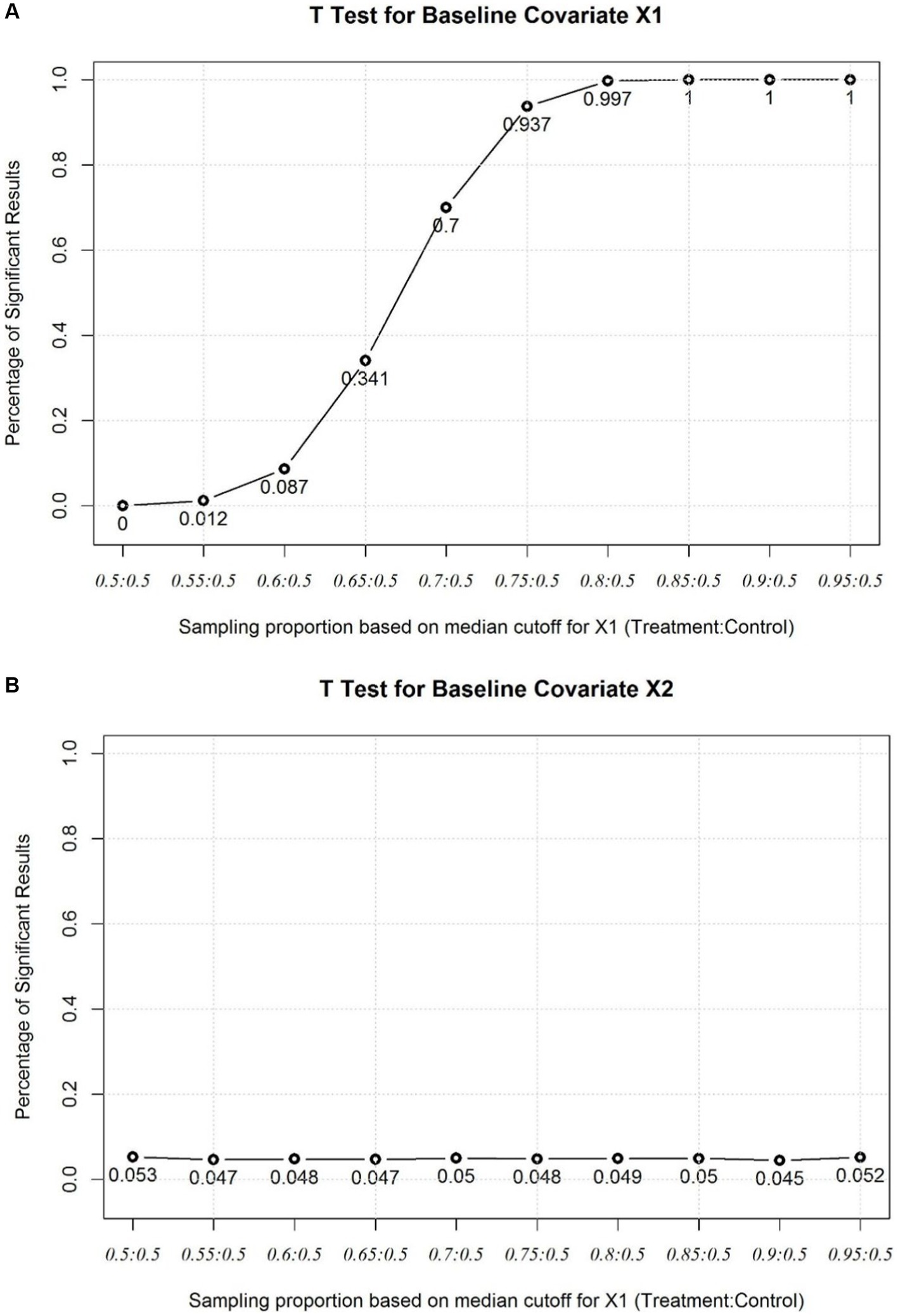
Figure 1. (A) Baseline T Test for the imbalanced covariate X1. (B) Baseline T Test for the balanced covariate X2.

Simulation 1: two normal covariate and linear regression setting

As the covariates are fully balanced, the type I error rates of all tests after adjusting for covariates maintain at baseline level. It may be noticing that approaches involve propensity score have slightly lower type I error rates. The possible reason for this is the extra variance introduced by propensity score approaches itself. As the covariates imbalance getting severe, the type I error rate of ANCOVA(x)-WRS gets inflated as the underlying ANCOVA assumption has been violated. The type I error rate of ANCOVA(p)-WRS has been much lower than ANCOVA(x)-WRS when covariates are severely imbalanced. It shows the impact of violation of ANCOVA assumption on type I error rate can be reduced by introducing propensity score because the propensity score is the conditional probability of receiving specific treatment for the observed covariates (Figure 2A). Even one or some covariates are severely imbalanced between groups, the propensity score could reduce the impact of the imbalance. When there is no covariates effect, the empirical powers of these test are close to 0.8 and JHM(x) has highest power. As covariates imbalance get severe, the empirical powers of tests involving covariate adjustment will decrease. The empirical powers of ANCOVA(p)-WRS and JHM(x) decrease slightly as covariate imbalance is severe, although as the empirical powers of AR(p5) decrease most to 0.6 (Figure 2B).

Figure 2

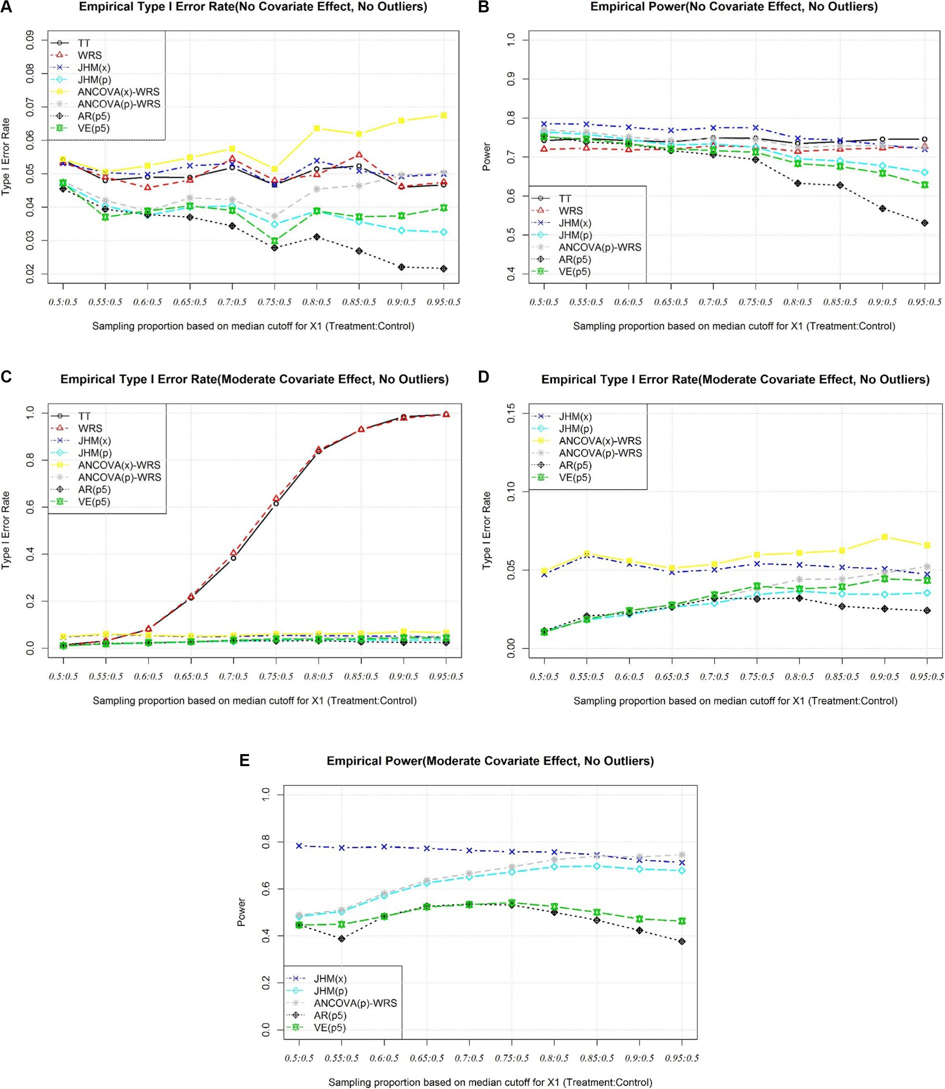
Figure 2. (A) Simulation 1, Empirical Type I Error Rate (No Covariate Effect). (B) Simulation 1, Empirical Power (No Covariate Effect). (C) Simulation 1, Empirical Type I Error Rate (Moderate Covariate Effect), All Approaches. (D) Simulation 1, Empirical Type I Error Rate (Moderate Effect), Selected Approaches. (E) Simulation 1, Empirical Power (Moderate Covariate Effect).

When there is true covariate effect, t test and Wilcoxon Rank Sum Test will have type I error rate inflated as covariates get imbalanced (Figure 2C). Like scenarios when there are no covariates effects, approaches involve propensity score have type I error rate lower than nominal level when covariates are fully balanced. Only the type I error rate of ANCOVA(x)-WRS gets inflated as covariate imbalance get severe (Figure 2D). When there are moderate covariates effects, the empirical power of propensity score approaches are much lower when covariates are fully balanced. As covariates imbalance get severe, the power of JHM(p) and the power of ANCOVA(p)-WRS get close level of JHM(x), although the two stratification approaches will still have lower power comparing to the other three valid approaches (Figure 2E).

Simulation 2: one strata variable and two normal covariate and linear regression setting

When covariates are fully balanced, the type I error rates are maintained at the nominal level.

As covariates imbalance get severe, AR(p5) inflates as covariate imbalance get severe (Figure 3A). It is not appropriate to use propensity score as a covariate in rank regression-based test. This suggest excluding strata variable is problematic. Three ANCOVA related approaches (ANCOVA(x)-WRS, ANCOVA(p)-WRS, and ANCOVA(p)2-WRS) also have inflation of type I error rate as covariate imbalance get severe as the ANCOVA assumption is violated (Figure 3A). JHM(x)-WRS also have type I error rate inflated as covariate imbalance get severe. One possible reason as covariate imbalance get severe, the covariates in two group do not share the same coefficient and adjust covariate effect based on Jaeckel’s Rank estimation may introduce bias to the adjusted response variable.

Figure 3

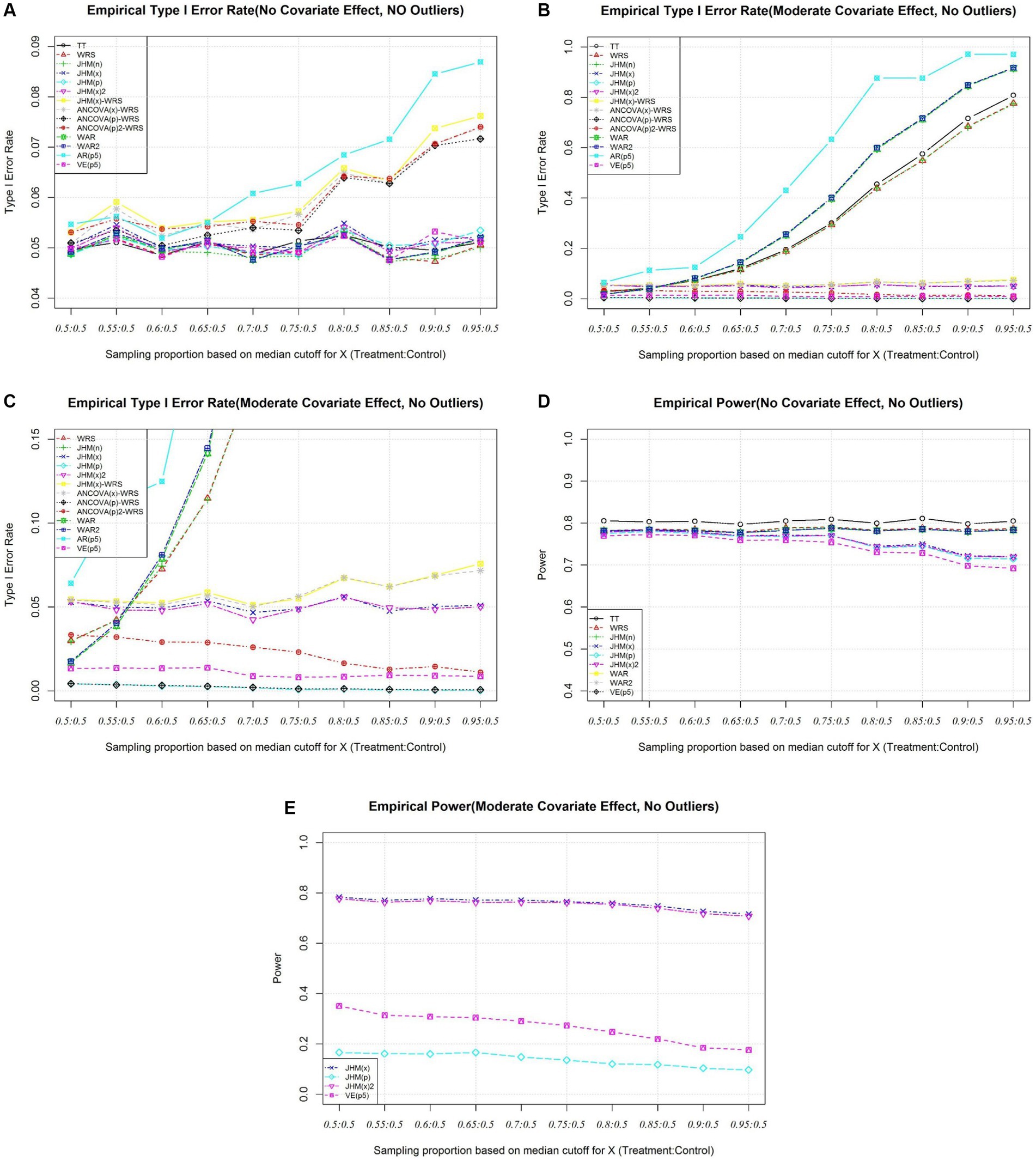
Figure 3. (A) Simulation 2, Empirical Type I Error Rate (No Covariate Effect). (B) Simulation 2, Empirical Type I Error Rate (Moderate Covariate Effect), All Approaches. (C) Simulation 2, Empirical Type I Error Rate (Moderate Effect), Selected Approaches. (D) Simulation 2, Empirical Power (No Covariate). (E) Simulation 2, Empirical Power (Moderate Covariate).

For other approaches, the type I error rate is maintained at nominal level (Figure 3A).

From Figure 3B, when there is true covariate effect, the type I error rates of approaches without adjust for covariate effects [TT, WRS, and JHM(n)] are inflated as covariates imbalance get severe. The type I error rate of two inverse weighted Hodges Lehmann estimator involved approach (WAR, WAR2) are inflated dramatically as covariate imbalance get severe. Inverse weighting approaches are problematic when covariate imbalance. The type I error rate of AR(p5) also inflates. This suggest the strata variable should be included in computing the propensity score. Besides, the type I error rate of ANCOVA(x)-WRS and JHM(x)-WRS also inflate as the assumptions are violated as covariate imbalance get severe. ANCOVA(p)-WRS and JHM(p) are conservative when there is true covariate effect. Only JHM(x) and JHM(x)2 maintain type I error rate at nominal level. JHM(x)2 align the strata effect before apply Jaeckel, Hettmansperger-McKean test (Figure 3C).

Under no covariate effect, the empirical power for the all the valid test statistics are presented in Figure 3D. The power is around 0.8 when the imbalance is not severe (Figure 3D). When there is a moderate covariate effect, the empirical power of JHM(x) and JHM(x)2 are also very close. Although the only valid propensity score approach, VE(p5) has empirical power only range from 0.4 to 0.2 as covariate imbalance get severe (Figure 3E).

Conclusion

It is problematic when the response variable is correlated with multiple covariates, and the covariates imbalance is severe. Propensity score could reduce the dimension of covariates into a scalar number. However, some tests after adjusting for propensity score approaches are invalid based on simulation result.

When quintile stratification of propensity score is applied to adjust for covariates effects, it is important to include all correlated covariates. Excluding a correlated imbalanced covariate would lead to the test to be invalid.

The type I error rates of proposed inverse propensity score weighting approaches inflate as covariates imbalance get severe. Propensity score could reduce the impact of covariate imbalance in ANCOVA adjusted Wilcoxon rank sum test. Also, propensity score could be treated as covariate in Jaeckel, Hettmansperger-McKean test. However, in both approaches, the power loss is dramatic comparing to non-propensity rank score approaches. Residuals after adjustments may induce correlation structure that makes the simulations of type I and power less accurate. Many of the issues observed after propensity score adjustments may be overcome with entropy balancing (22).

Data availability statement

The original contributions presented in the study are included in the article/supplementary material, further inquiries can be directed to the corresponding author.

Author contributions

JY: Conceptualization, Formal analysis, Methodology, Software, Visualization, Writing – original draft. DL: Conceptualization, Investigation, Methodology, Project administration, Resources, Supervision, Writing – review & editing.

Funding

The author(s) declare that no financial support was received for the research, authorship, and/or publication of this article.

Conflict of interest

JY was employed by Merck and Co., Inc.

The remaining author declares that the research was conducted in the absence of any commercial or financial relationships that could be construed as a potential conflict of interest.

Publisher’s note

All claims expressed in this article are solely those of the authors and do not necessarily represent those of their affiliated organizations, or those of the publisher, the editors and the reviewers. Any product that may be evaluated in this article, or claim that may be made by its manufacturer, is not guaranteed or endorsed by the publisher.

References

1. European Medicines Agency. Committee for Medicinal Products for Human Use. Guideline on adjustment for baseline covariates in clinical trials. London: European Medicines Agency (2015).

Google Scholar

2. Center for Drug Evaluation and Research. Draft guideline on adjusting for covariates in randomized clinical trials for drugs and biologics with continuous outcomes. Montgomery: Food and Drug Administration (2019).

Google Scholar

3. Center for Drug Evaluation and Research. Adjusting for covariates in randomized clinical trials for drugs and biological products. Montgomery: Food and Drug Administration (2021).

Google Scholar

4. Center for Drug Evaluation and Research. Adjusting for covariates in randomized clinical trials for drugs and biological products. Montgomery: Food and Drug Administration (2023).

Google Scholar

5. Freedman, DA . On regression adjustments in experiments with several treatments. Ann Appl Stat. (2008) 2:176–96. doi: 10.1214/07-AOAS143

Crossref Full Text | Google Scholar

6. Rosenbaum, PR, and Rubin, DB. The central role of the propensity score in observational studies for causal effects. Biometrika. (1983) 70:41–55. doi: 10.1093/biomet/70.1.41

Crossref Full Text | Google Scholar

7. Zeng, S, Li, F, Wang, R, and Li, F. Propensity score weighting for covariate adjustment in randomized clinical trials. Stat Med. (2021) 40:842–58. doi: 10.1002/sim.8805

Crossref Full Text | Google Scholar

8. Imai, K, and Ratkovic, M. Covariate balancing propensity score. J R Stat Soc B Statist Methodol. (2014) 76:243–63. doi: 10.1111/rssb.12027

Crossref Full Text | Google Scholar

9. McCaffrey, DF, Ridgeway, G, and Morral, AR. Propensity score estimation with boosted regression for evaluating causal effects in observational studies. Psychol Methods. (2004) 9:403–25. doi: 10.1037/1082-989X.9.4.403

PubMed Abstract | Crossref Full Text | Google Scholar

10. Setoguchi, S, Schneeweiss, S, Brookhart, MA, Glynn, RJ, and Cook, EF. Evaluating uses of data mining techniques in propensity score estimation: a simulation study. Pharmacoepidemiol Drug Saf. (2008) 17:546–55. doi: 10.1002/pds.1555

PubMed Abstract | Crossref Full Text | Google Scholar

11. Rosenbaum, PR . Covariance adjustment in randomized experiments and observational studies. Stat Sci. (2002) 17:286–327. doi: 10.1214/ss/1042727942

Crossref Full Text | Google Scholar

12. Cochran, WG . The effectiveness of adjustment by subclassification in removing bias in observational studies. Biometrics. (1968) 24:295–313. doi: 10.2307/2528036

PubMed Abstract | Crossref Full Text | Google Scholar

13. Abadie, A, Drukker, D, Herr, JL, and Imbens, GW. Implementing matching estimators for average treatment effects in Stata. Stata J. (2004) 4:290–311. doi: 10.1177/1536867X0400400307

Crossref Full Text | Google Scholar

14. Rosenbaum, PR . Model-based direct adjustment. J Am Stat Assoc. (1987) 82:387–94. doi: 10.1080/01621459.1987.10478441

Crossref Full Text | Google Scholar

15. Lee, BK, Lessler, J, and Stuart, EA. Improving propensity score weighting using machine learning. Stat Med. (2010) 29:337–46. doi: 10.1002/sim.3782

PubMed Abstract | Crossref Full Text | Google Scholar

16. Austin, PC . A critical appraisal of propensity-score matching in the medical literature between 1996 and 2003. Stat Med. (2008) 27:2037–49. doi: 10.1002/sim.3150

PubMed Abstract | Crossref Full Text | Google Scholar

17. D'Agostino, RB Jr . Propensity score methods for bias reduction in the comparison of a treatment to a non-randomized control group. Stat Med. (1998) 17:2265–81. doi: 10.1002/(SICI)1097-0258(19981015)17:19<2265::AID-SIM918>3.0.CO;2-B

PubMed Abstract | Crossref Full Text | Google Scholar

18. Mann, HB, and Whitney, DR. On a test of whether one of two random variables is stochastically larger than the other. Ann Math Stat. (1947) 18:50–60. doi: 10.1214/aoms/1177730491

Crossref Full Text | Google Scholar

19. Wilcoxon, F . Individual comparisons by ranking methods. Biom Bull. (1945) 1:80–3. doi: 10.2307/3001968

Crossref Full Text | Google Scholar

20. Jaeckel, LA . Estimating regression coefficients by minimizing the dispersion of the residuals. Ann Math Stat. (1972) 43:1449–58. doi: 10.1214/aoms/1177692377

Crossref Full Text | Google Scholar

21. McKean, JW, and Hettmansperger, TP. Tests of hypotheses based on ranks in the general linear model. Commun Stat Theory Methods. (1976) 5:693–709. doi: 10.1080/03610927608827388

Crossref Full Text | Google Scholar

22. Hainmueller, J . Entropy balancing for causal effects: a multivariate reweighting method to produce balanced samples in observational studies. Polit Anal. (2012) 20:25–46. doi: 10.1093/pan/mpr025

Crossref Full Text | Google Scholar