Multivariate realized volatility: an analysis via shrinkage methods for Brazilian market data

1 Introduction

Understanding volatility has become fundamental for option pricing, portfolio selection and risk management. Historically, the Finance and Econometrics literature has concentrated efforts and developed the most diverse methodologies in the construction of better measures for this purpose. However, two problems are intrinsic to the discussion: the fact that true volatility cannot be observed and needs to be estimated [1] and the dimensionality problem of the multivariate realized variance matrix [2, 3].

The evolution of portfolio selection theory has underscored the necessity for more efficient and robust methods in estimating the Covariance Matrix [3], proving fundamental in comprehending the dynamics governing asset return behavior. Concurrently, technological advancements and the growth of the financial market have facilitated the creation of more companies and an influx of data. Practices developed at the intersection of statistics and computing, particularly involving large databases, have become indispensable components in financial applications. This signifies a paradigm shift in information management and alters our understanding of the decision-making process: volatility is now perceived as dynamic and less parsimonious, deviating from suggestions in earlier literature [3, 4].

The availability of high-frequency data enables the construction of the realized covariance matrix, serving as a proxy for the latent true volatility [5]. Notably, there is a dearth of literature addressing this issue using penalty methods specifically tailored for data from emerging markets, characterized by lower liquidity (e.g., [6, 7]) and making the usual estimation of the variance matrix carried out in higher dimensions more difficult. Moreover, the incorporation of penalties allows us to tackle the dimensionality problem, a significant impediment in multivariate volatility literature due to computational complexity.

The objective of this study is to estimate multivariate volatility models utilizing high-frequency data from the Brazilian market, employing shrinkage methods from the Machine Learning literature (e.g., [3, 8, 9]). We introduced a flexible algorithm for estimating the covariance matrix, deliberately avoiding the use of sample covariance. Additionally, the most suitable regularization approach, whether ℓ₁, ℓ₂, or a combination of both norms, is selected based on predictive performance, using the Model Confidence Set (MCS) mechanism, proposed in Hansen et al. [10].

Through the proposed exercise, we aim to investigate how volatilities are governed in a multivariate context for the most liquid assets on the Brazilian stock exchange, employing a computationally efficient methodology. Additionally, the study seeks to determine whether a specific sector of the economy is correlated with others. Questions regarding whether asset variances are influenced by past dynamics or spillover-type effects, and whether there exist disparities in the dynamics of variance and covariance, will be explored. It is crucial to highlight that despite challenges posed by issues such as market microstructure noise and the structure of our data, the primary objective of this work is to estimate the covariance matrix for a substantial volume of assets.

The structure of the work is divided into five sections, starting with this introduction. Section 2 provides a literature review, while Section 3 outlines the methodology. The empirical analysis is presented in Section 4, and the study concludes with Section 5.

2 Literature review

The literature review seeks to connect seminal works on covariance matrix utilization and estimation in finance, alongside primary references on conditional variance and realized variance models. Drawing from the finance literature, we revisit the seminal work of Markowitz [11], which laid the groundwork for estimating variance and covariance matrices between assets. After we delve into the volatility models introduced by Bollerslev [12], examining the maturity of this field, the performance of univariate models, and the practical challenges encountered in multivariate models. Additionally, we explore an extensive literature on the estimation of high-dimensional covariance matrices. Lastly, we discuss the work of Fleming et al. [13], which provides economic justification for utilizing high-frequency data, and Ledoit and Wolf [3] which reviews the use of shrinkage methods in realized variance estimation.

Markowitz's [11] contribution revolves around portfolio selection. The study analytically demonstrates that the risk of a portfolio is not solely determined by the average of individual risks; rather, it necessitates consideration of the correlation between assets. This foundational work systematized the understanding of diversification behavior among economic agents. At the time of its publication, asset risk was measured by the standard deviation of its return. In this theory, asset returns are treated as random variables, and the investor's objective is to optimally allocate weights to each asset. Within this theoretical framework, the optimal choice is determined by a vector of weights that minimizes portfolio variance.

Let r_i be the rate of return associated with asset i, where i = 1, …, n. The vector of returns is denoted by z, such that z is a n × 1 vector. Additionally, let's assume μ_i = 𝔼(r_i), $\text{m}={\left({\mu }_1,{\mu }_2,\dots ,{\mu }_n\right)}^{\prime }$ and cov(z) = Σ. If $\text{w}={\left(w_1,w_2,\dots ,w_n\right)}^{\prime }$ is the set of weights associated with the portfolio, then the rate of return $r=\sum _{i=1}^n{r}_i{w}_i$ is, analogously, a random variable with mean m′w and variance w′Σw. Let μ_b be the investor's baseline rate of return, then an optimal portfolio is any combination of assets that solves the following problem:

$\begin{array}{l}{\displaystyle \underset{\text{w}}{min}}\{{\text{w}}^{\prime }\Sigma \text{w}\}\\ s.t.:\\ {\text{m}}^{\prime }\text{w}\ge {\mu }_b\\ {\text{e}}^{\prime }\text{w}=1\end{array}$

In this context, e represents a vector of dimensions n × 1, with all elements set to 1. The significance of this theoretical framework is noteworthy, as it laid the foundation for measuring the volatility of an asset. Subsequently, the construction of covariance matrices and the study of correlations have become pivotal in portfolio construction, risk management, and option pricing.

A limitation in applying the Markowitz method is its static nature, as it is usually estimated using unconditional covariance. However, a stylized fact in financial series is the presence of conditional variance structures. Engle [14] presents the seminal work on estimating variance through the Autoregressive Conditional Heteroscedasticity (ARCH) model. This marks the inception of models designed for volatility estimation, motivated by empirical observations of financial series properties. Notably, the model emphasizes the greater importance of modeling the variance autocorrelation structure compared to the average dependence structure. The model's specification is given by:

$\begin{array}{l}{y}_t=u_t\\ u_t~\mathcal{N}\left(0;{\sigma }_t^2\right)\\ {\sigma }_t^2={\alpha }_0+{\displaystyle \sum _{i=1}^q}{\alpha }_j{u}_{t-j}^2\end{array}$

In this formulation, u_t represents a disturbance term, and ${\sigma }_t^2$ denotes the return variance conditioned on past information. The parameter α₀ is an intercept and parameters α_j measures de dependence of conditional variance on past squared returns. The emergence of the ARCH model aimed to introduce a new class of stochastic processes with zero mean, serially non-autocorrelated, and non-constant conditional variances when conditioned on past information. The suggested estimation method for this model is the maximum likelihood method.

Despite the effectiveness and simplicity of the ARCH(q) model, it exhibits a variance memory that extends up to lag q. This implies that a process demonstrating higher memory in variance would necessitate the estimation of a larger model. A natural solution to this challenge was to specify the model with lags of the variance itself:

$\begin{array}{l}{\sigma }_t^2={\alpha }_0+{\displaystyle \sum _{i=1}^q}{\alpha }_i{u}_{t-i}^2+{\displaystyle \sum _{i=1}^p}{\beta }_i{\sigma }_{t-i}^2\end{array}$

This solution was proposed by Bollerslev [12], introducing a generalized ARCH(p) specification known as the Generalized Autoregressive Conditional Heteroskedasticity - GARCH(p, q) model with the new parameters β_i measuring the dependence of conditional volatility on past values of itself. Subsequent developments in the literature focused on adapting this model, leading to the establishment of a family of GARCH models [15].

In Bollerslev et al. [16], a paradigm shift occurs with the restructuring of the Capital Asset Pricing Model (CAPM) in the conditional volatility context. In the original CAPM, asset prices are linked to return uncertainty, and the premium to incentivize investors is proportionate to non-diversifiable risk, measured by the covariance of the asset's return with the return of the market portfolio. Analyzing US government bond and equity data, Bollerslev et al. [16] show that the conditional covariance is found to be slightly time-varying and a significant determinant of the risk premium. Additionally, the implicit betas are also observed to be time-variant.

Hansen and Lunde [17] subsequently confirm the viability of GARCH(1, 1) by estimating 330 alternative models. They demonstrate, using data on American exchange rates and stock returns from International Business Machines Corporation (IBM), the model's superior predictive capacity and its parsimonious, computationally efficient structure. However, the natural extension of these models the multivariate version did not gain the same reputation due to a practical setback: multivariate volatility models face computational challenges stemming from the dimensional problem, later formalized in the literature as the curse of dimensionality. The models suggested by the literature are presented in Martin et al. [18].

The multivariate extension of volatility models encounters two fundamental problems: (i) the covariance matrix between assets must be positive definite, and (ii) the number of unknown parameters governing variances and covariances grows exponentially with the model size (number of series). The four principal GARCH multivariate models [19] are:

• The VECH model, a generalization of GARCH(p, q) for the multivariate universe.

• The BEKK model [20], which reduces the dimension computed in VECH and imposes the mathematical restriction that the covariance matrix be positive definite.

• The DCC model [21], which further reduces the size of BEKK models, making the use of larger dimensions more feasible.

• The DECO model [22], which simplifies the DCC specification by constraining contemporary correlations to be numerically identical.

Another way to model variance is through the formulation derived from continuous-time stochastic processes, using the concept of Realized Variance (RV) [4, 23–25]. Realized variance is a measure of the variation in asset prices observed over a given time period. It is computed as the sum of squared high-frequency returns over that period. This measure is popular because it uses intraday data, providing more accurate estimates of volatility compared to traditional daily measures.

The connection between realized variance and continuous-time stochastic processes arises when we consider the limit as the sampling frequency of returns approaches infinity. In this limit, realized variance can be related to the integral of the instantaneous variance process over time. This concept naturally extends to the multivariate case, giving rise to the concept of realized covariances. However, the same estimation difficulty exists when the number of assets is high, analogous to the estimation problem of multivariate GARCH models, as discussed in Bollerslev et al. [2].

In the empirical literature, substantial efforts have been dedicated to resolving the dimensional problem, with numerous works focused on the estimation of high-dimensional covariance matrices. Some of the noteworthy contributions include refs. [26–29]. Among these, two works stand out as significant references: Medeiros et al. [30] and Alves et al. [31].

In Medeiros et al. [30], the authors addressed the modeling and prediction of high-dimensional covariance matrices using data from 30 assets in the Dow Jones. They employed a penalized VAR estimation, considering Least Absolute Shrinkage and Selection Operator (LASSO) type estimators to mitigate the dimensional problem. A survey on the use of shrinkage methods is this class of problems can be found in Ledoit and Wolf [3]. Medeiros et al. [30] show that the covariance matrix could be predicted nearly as accurately as when the true dynamics governing the series are known. The data, aggregated daily at 5-min intervals, spans from 2006 to 2012.

Addressing the dimensional problem more comprehensively, Alves et al. [31] extended the exercise to all 500 assets of the S&P 500 on a daily basis. The approach involved estimating a sparse covariance matrix based on a factor decomposition at the company level (size, market value, profit generation) and sectoral restrictions on the residual covariance matrix. The restricted model was estimated using the Vector Heterogeneous Autoregressive model (VHAR), penalizing variable selection through LASSO. This exercise led to improved estimates of minimum variance portfolios.

Following the factor model [32], the excess return on an asset i, r_i,t, satisfies:

$\begin{array}{l}{r}_{i,t}={\beta }_{i1,t}{f}_{1,t}+\cdots +{\beta }_{iK,t}{f}_{K,t}+{\epsilon }_{i,t}\end{array}$

Here, f_1,t, …, f_K,t denote the excess returns of K factors, β_ik,t, k = 1, …, K, represent the marginal effects, and ε_i,t is the error term. For the active N, the set of equations can be expressed in matrix format as ${\text{r}}_t={\text{B}}_t^{\prime }{\text{f}}_t+{\epsilon }_t$. It is assumed that 𝔼(ε_t|f_t) = 0. The factors utilized are linear combinations of assets, forming short- and long-term stock portfolios based on idiosyncratic and sectoral characteristics.

The authors initiate by decomposing the covariance matrix into two components: a matrix of factors and a second residual matrix. Let Σ_t be the realized covariance matrix of returns at time t, i.e., Σ_t = cov(r_t). Building on the earlier considerations, this can be expressed as:

$\begin{array}{l}{\Sigma }_t=\text{cov}\left({\text{B}}_t^{\prime }{\text{f}}_t\right)+\text{cov}\left({\epsilon }_t\right)\\ ={\text{B}}_t^{\prime }{\Sigma }_{\text{f},t}{\text{B}}_t+{\Sigma }_{\epsilon ,t}\end{array}$

In a theoretical and practical context, Ledoit and Wolf [33] highlighted the risks associated with using the sample covariance matrix for portfolio optimization. The estimation errors in the sample covariance matrix are more likely to disrupt the mean-variance optimizer. They propose replacing the sample covariance matrix with a transformation known as shrinkage. This approach computes estimates that moderate extreme values toward central values, systematically reducing estimation errors where they have a more significant impact. Statistically, this is achieved through the challenge of determining the intensity of shrinkage, the rationale for which is presented in the paper.

Finally, Fleming et al. [13] provides justification for utilizing high-frequency data. Drawing from recent literature, they empirically investigate whether there are precision gains in daily volatility estimates from intraday data. The authors analyze the economic value of realized volatility in an investor decision-making context. The results indicate substantial improvements when replacing daily data estimates with intraday data estimates: a risk-averse investor would be willing to pay 50 to 200 basis points per year to capture the gains observed in portfolio performance. Furthermore, these gains are found to be robust even when accounting for transaction costs.

3 Methodology

As in Medeiros et al. [30] and Alves et al. [31], we represent the covariance matrix at time instant t as Σ_t. Each entry of the matrix is potentially a function of past entries, and we express Σ_t as a function of Σ_t−1, …, Σ_t−p. Formally:

$\begin{array}{ll}{\text{y}}_t=\omega +{\displaystyle \sum _{i=1}^p}{\beta }_i{\text{y}}_{t-i}+{ϵ}_t& (1)\end{array}$

y_t = vech(Σ_t), where vech(·) is the vectorization operation, transforming Σ_t into a column vector of unique entries. β_i, i = 1, …, p, is the matrix that captures the dynamics between Σ_t and its past, ϵ_t is an error term and ω is a vector of constants. It is, therefore, an Autoregressive Vector structure, of order p- VAR(p).

For a covariance matrix of n assets, there will be n(n + 1)/2 distinct entries. A VAR(p) process in this case would imply a total of n(n + 1)(p + 1)/2 parameters. In other words, both in calculating the matrix and in specifying the VAR, there would be issues with dimensionality, as in both exercises, the number of parameters grows exponentially. Additionally, this configuration results in a greater number of potential predictors than observations—high dimensionality. Tibshirani et al. [34] demonstrate that in this scenario, traditional estimation via OLS implies overfitting, and there is a specification error as the solution will not be unique.

In Laurini and Ohashi [35], there is a discussion regarding the limitations of using the sample covariance matrix for dependent processes. In intraday scenarios, the return series tend to be more dependent compared to larger temporal aggregations. Additionally, due to market microstructure noise, the observed price is not the true price, introducing measurement error. Assuming that P_t is the intraday price of a generic asset:

$\begin{array}{l}{P}_t=P_t^V+{\eta }_t\end{array}$

$P_t^V$ is the true price value and η_t is the measurement error. Note that:

$\begin{array}{l}{P}_t-P_{t-1}=P_t^V+{\eta }_t-P_{t-1}\\ \Delta P_t=P_t^V+{\eta }_t-P_{t-1}^V-{\eta }_{t-1}\\ =\Delta P_t^V+{\eta }_t-{\eta }_{t-1}\end{array}$

The first difference in the series generates MA(1) type contamination.

Our work aims to address challenges in both stages of the analysis: the need to calculate Σ_t prior to estimation, and the subsequent estimation process itself. As demonstrated, relying on the sample covariance for these tasks may not be optimal. We propose a flexible framework that allows for the specification of various alternatives to sample covariance when handling data. We later formalize an equation-by-equation estimation approach for Equation (1), particularly suitable for high dimensions, using traditional models from the Machine Learning literature [8, 9, 36].

As discussed in Ledoit and Wolf [33], the use of sample covariance can be detrimental for portfolio optimization purposes. This stylized fact is documented in Jobson and Korkie [37]. The conventional approach of collecting historical return data and generating the sample covariance matrix is sensitive to the number of assets, leading to substantial estimation errors. This implies that larger prediction errors in extreme coefficients of the matrix result in larger values, influencing optimization problems with greater weights on these coefficients. This phenomenon is known as error-maximization, as discussed in Michaud [38].

In Fan et al. [39], a comprehensive review of methods for estimating high-dimensional covariance and precision matrices is presented. Similar to the numerical problem mentioned earlier, high-dimensional matrices become singular, making them non-invertible. The aggregation of estimation errors in high dimensions has significant impacts on accuracy. Motivated by these challenges, the authors categorize estimation strategies. Modern practice involves consistent estimations based on regularization, assuming the matrix of interest is sparse.

For this estimation, an ℓ₁ penalty is applied to the maximum likelihood function. In such an approach, a non-convex penalty can be imposed to reduce bias. On the other hand, there is a complementary literature based on approaches related to the rank of the matrix. These methods make the data distribution more flexible for a non-Gaussian scenario with heavy tails, common in financial series. However, sparsity is not always empirically reasonable, especially in economic data. To address this, the class of models based on conditional sparsity is considered, where common factors are used, and it is assumed that the covariance matrix of the remaining components is sparse.

To allow flexibility, we will leverage [40]. This library provides various methods for calculating Σ_t. In addition to avoiding the use of sample covariance, employing multiple methods can enhance robustness in estimations. The following describes the structures we will employ:

• Matrix of type ewma: We compute the covariance matrix based on Exponential Weighting Moving Average (EWMA), documented in the traditional RiskMetrics methodology [41]. Formally, the covariance matrix is denoted by the matrix and a constant 0 < λ < 1, such that:

${\Sigma }_{t+1}=\lambda {\Sigma }_t+\left(1-\lambda \right){\text{r}}_t{{\text{r}}^{\prime }}_t.$

Considering a sample of N assets, r_t is a vector N × 1 of returns at time t. By convention we adopt λ = 0.94.

• Matrix of type color: The color matrix estimation strategy involves a weighted average of the sample covariance matrix and a shrinkage target. In this specific approach, the shrinkage target is characterized by a constant correlation structure between pairs. This method is introduced and defined in Ledoit and Wolf [33].

Let S be the sample covariance matrix and F be a structured estimator. The idea is to propose a convex combination δF + (1 − δ)S, such that 0 < δ < 1. It is a shrinkage technique in that we “shrink” S in the direction of F. δ is known as shrinkage constant. To introduce F, we will have the following notation, as in the original work: let y_it, 1 ≤ i ≤ N, 1 ≤ t ≤ T. The analysis will assume that returns are independent and identically distributed over time and with finite fourth moments. Here, ${ȳ}_i=T^{-1}\sum _{i=1}^T{y}_{it}$. Define that Σ is the true covariance matrix and S is the sample covariance matrix. We will have that σ_ij represents the inputs of Σ and that s_ij represents the inputs of S. The population and sample correlations are, respectively:

$\begin{array}{l}{{\rho }_{i,j}}_{\Sigma }=\frac{{\sigma }_{ij}}{\sqrt{{\sigma }_{ii}{\sigma }_{jj}}}\\ {{\rho }_{i,j}}_S=\frac{s_{ij}}{\sqrt{s_{ii}{s}_{jj}}}\end{array}$

Additionally, we can take the average of such measurements:

$\begin{array}{l}{\bar{\rho }}_{\Sigma }=\frac{2}{\left(N-1\right)N}{\displaystyle \sum _{i=1}^{N-1}}{\displaystyle \sum _{j=i+1}^N}{{\rho }_{i,j}}_{\Sigma }\\ {\bar{\rho }}_S=\frac{2}{\left(N-1\right)N}{\displaystyle \sum _{i=1}^{N-1}}{\displaystyle \sum _{j=i+1}^N}{{\rho }_{i,j}}_S\end{array}$

The matrix F, defined as shrinkage target, will have diagonal and off-diagonal input, respectively:

$\begin{array}{l}{f}_{ii}=s_{ii}\\ f_{ij}={\bar{\rho }}_S\sqrt{s_{ii}{s}_{jj}}\end{array}$

Finally, we find δ from an optimization problem. Here, the loss function to be optimized is intuitive and does not require the inverse of S: it is the quadratic distance between the true covariance matrix and the estimated one, based on the Frobenius norm. The Frobenius norm of a symmetric matrix N × N of entries z_ij is defined by $\left|\right|Z|{|}^2=\sum _{i=1}^N\sum _{j=1}^N{z}_{ij}^2$. The objective is to find the shrinkage constant that minimizes the expected value below:

$\begin{array}{l}{\widehat{\delta }}^{*}= arg min\{𝔼{\left(\left|\right|\delta F+\left(1-\delta \right)S-\Sigma \left|\right|\right)}^2\}\end{array}$

• Matrix of type large: this is the estimator proposed in Ledoit and Wolf [42]. Here, we have that the shrinkage target is given by a one-factor model. The factor is equal to the cross-sectional average of all variables. The weight, also called shrinkage intensity, is chosen based on the minimization of the quadratic loss, measured by the Frobenius norm. This is a method more suitable for high dimensions and, additionally, it is well conditioned in the sense that the inversion is guaranteed (non-singular matrix) and we are not induced into estimation errors. This is a regularization in the eigenvalues of the matrix in such a way that the eigenvalues are forced toward more central values. Here, the objective is to find

$\begin{array}{l}{\Sigma }^{*}={\rho }_1\text{I}+{\rho }_{2}S\end{array}$

which minimizes 𝔼(||Σ^* − Σ||²). I is the identity matrix, S = XX′/n is the sample covariance matrix, where X is a p × n matrix of n independent and identically distributed observations with zero mean and variance Σ. In the original work, under finite samples, the authors formulate the following problem:

$\begin{array}{l}{\displaystyle \underset{{\rho }_1,{\rho }_2}{min}}𝔼(||{\Sigma }^{*}-\Sigma |{|}^2)\\ s.t.:{\Sigma }^{*}={\rho }_1\text{I}+{\rho }_{2}S\end{array}$

The solution is given by:

$\begin{array}{l}{\Sigma }^{*}=\frac{{\beta }^2}{{\delta }^2}\mu \text{I}+\frac{{\alpha }^2}{{\delta }^2}S\\ 𝔼(||{\Sigma }^{*}-\Sigma |{|}^2)=\frac{{\alpha }^2{\beta }^2}{{\delta }^2}\\ \mu =\langle \Sigma ,\text{I}\rangle \\ {\alpha }^2=||\Sigma -\mu \text{I}|{|}^2\\ {\beta }^2=𝔼(||S-\Sigma |{|}^2)\\ {\delta }^2=𝔼(||S-\mu \text{I}|{|}^2)\end{array}$

Our approach to estimate Equation (1) involves an equation-by-equation estimation using the library developed by Friedman et al. [43]. In contrast to the methodologies proposed in our reference works [30, 31], our strategy establishes a flexible structure. This structure, based on the predictive performance of a model class, dynamically determines whether the estimation should be conducted via Ridge Regression [44], LASSO [45], or Elastic Net [46].

The flexibility of our approach allows us to adapt the estimation technique to the characteristics of each equation, optimizing the trade-off between model complexity and predictive accuracy. By incorporating Ridge, LASSO, or Elastic Net regularization, our methodology aims to enhance the robustness and accuracy of the covariance matrix estimation for each individual equation within the multivariate context.

Let y_i be an element of Σ_t and x_i be the set that contains the lagged Σ_t. The estimation strategy consists of solving:

$\begin{array}{ll}{\displaystyle \underset{{\beta }_0,\beta }{min}}\{\frac{1}{N}{\displaystyle \sum _{i=1}^N}{w}_{i}l\left(y_i,{\beta }_0+{\beta }^{\prime }{x}_i\right)+\lambda [\left(1-\alpha \right)||\beta |{|}_2^2/2+\alpha ||\beta |{|}_1]\}& (2)\end{array}$

This is a General Linear Model with a penalized maximum likelihood structure. In Equation (2), N is the number of temporal observations, λ is a tuning parameter and l(·) is the contribution of observation i to the log function. likelihood. Here, 0 ≤ α ≤ 1, such that we will have a LASSO type specification if α = 1, Ridge for α = 0 and Elastic Net for 0 < α < 1.

The Ridge mechanism is unique in that it does not perform variable selection; a set of correlated covariates will have numerically close coefficients. This estimator has a closed-form solution, as it involves solving a quadratic programming problem. In LASSO, there is the possibility of variable selection, reducing the dimensionality of the problem. On the other hand, Elastic Net is a hybrid structure, incorporating both ℓ₁ regularization from LASSO and ℓ₂ regularization from Ridge Regression. The algorithms in the glmnet library use cyclic coordinate descent, which successively optimizes the objective function over each parameter with fixed others and switches repeatedly until convergence. The package also makes use of strict rules for efficiently restricting the active set.

Our starting point involves a specification assuming Gaussian errors. This formulates our problem as:

$\begin{array}{ll}{\displaystyle \underset{{\beta }_0,\beta }{min}}\{\frac{1}{2N}{\displaystyle \sum _{i=1}^N}{\left(y_i-{\beta }_0-x_i^{\prime }\right)}^2+\lambda [\left(1-\alpha \right)||\beta |{|}_2^2/2+\alpha ||\beta |{|}_1]\}& (3)\end{array}$

λ ≥ 0 is traditionally found by cross-validation. However, we did not choose to solve the problem in this way. The use of cross-validation is not recommended in problems involving time series, due to the dependency structure. Therefore, we will start with an adaptation of the library and find λ using an information criterion. Three criteria are used in the literature:

$\begin{array}{l}\text{AIC}=2k-2ln\widehat{L}\\ \text{BIC}=klnn-2ln\widehat{L}\\ \text{HQ}=-2\widehat{L}+2kln\left(lnn\right)\end{array}$

Where n is the number of observations, k is the number of parameters and $\widehat{L}$ is the maximum value of the likelihood function. In Hamilton [47] we find the following relationship, for n ≥ 16:

$\begin{array}{l}\text{BIC}\le \text{HQ}\le \text{AIC}\end{array}$

In other words, HQ is an intermediate information criterion, while AIC is the most flexible and BIC is the most rigorous, that is, it penalizes the inclusion of variables in the model more severely. In our exercise we chose the Hannan-Quinn (HQ) criterion. This adaptation is implemented in the function ic.glmnet.¹

As previously stated:

• If α = 0, we solve the following problem:

$\begin{array}{l}{\displaystyle \underset{{\beta }_0,\beta }{min}}\{\frac{1}{2N}{\displaystyle \sum _{i=1}^N}{\left(y_i-{\beta }_0-x_i^{\prime }\right)}^2+\lambda ||\beta |{|}_2^2/2\}\end{array}$

This is the structure of a Ridge Regression. Note that if λ = 0, we would be in a traditional Least Squares problem. Additionally, it is possible to demonstrate that if $\widehat{\beta }$ solves the above problem, then $\underset{\lambda \to \infty }{lim}\widehat{\beta }=0$.

• If α = 1, we solve the following problem:

$\begin{array}{l}{\displaystyle \underset{{\beta }_0,\beta }{min}}\{\frac{1}{2N}{\displaystyle \sum _{i=1}^N}{\left(y_i-{\beta }_0-x_i^{\prime }\right)}^2+\lambda ||\beta |{|}_1\}\end{array}$

This is the structure of the LASSO method, which is a shrinkage method. When we are faced with a scenario of high values, we can select variables via LASSO and, additionally, produce sparse solutions. In other words, it is possible to perform a dimension reduction in the problem, finding a matrix of coefficients that uses fewer features (predictors) than a traditional Least Squares solution or via Ridge. Finally, as we can see in Tibshirani et al. [34], in finite samples we have good performance and avoid the classic trade-off problem of bias and variance.

• If 0 < α < 1, we solve the following problem:

$\begin{array}{l}{\displaystyle \underset{{\beta }_0,\beta }{min}}\{\frac{1}{2N}{\displaystyle \sum _{i=1}^N}{\left(y_i-{\beta }_0-x_i^{\prime }\right)}^2+\lambda [\left(1-\alpha \right)||\beta |{|}_2^2/2+\alpha ||\beta |{|}_1]\}\end{array}$

This is the structure of Elastic Net, according to Zou and Hastie [46]. This is a hybrid formulation, in which both ℓ₁ and ℓ₂ penalties are computed. This format is beneficial and appears in the literature as an answer to some theoretical limitations that are a consequence of LASSO: (i) LASSO in a high-dimensional scenario, that is, more predictors (k) than observations (n), has the ability to select a maximum of n variables, (ii) for variables that, in pairs, are highly correlated, LASSO will only select one of them and (iii) in high dimension, for highly correlated features, the predictive performance in Ridge Regression is superior to LASSO.

Since our structure is flexible, we will require a method of choosing the model based on some criteria. In this work we will propose the Model Confidence Set (MCS) algorithm, proposed in Hansen et al. [10]. The idea is to start from a discrete grid, such that α_grid = [0.0, 0.1, 0.2, 0.3, 0.4, 0.5, 0.6, 0.7, 0.8, 0.9, 1]. That is, we will, by equation, estimate (Equation 3), take a α ∈ α_grid and evaluate the “winning” model based on predictive performance. We separated 20% of the sample to establish a training set and test set. That is, 20% of the data was excluded from the sample to compute the predictive performance.

MCS involves building a set of models such that the best model, from a predictive point of view, is an element of this set given a level of confidence. It is an algorithm that sequentially tests the null hypothesis that the models have identical accuracy. Based on an elimination criterion, it selects the best model or set of models. It is, therefore, an inferential way of selecting models, as it is based on global methods, unlike evaluating specific measurements. To implement MCS we will rely on Bernardi and Catania [48]. Let Y_t be our time series at time instant t and Ŷ_i,t be the fit of model i, at t. The first step is to define a loss function ℓ_i,t that is associated with the ith model, such that:

$\begin{array}{l}{\ell }_{i,t}=\ell \left(Y_t,{Ŷ}_{i,t}\right)\end{array}$

The procedure is started from a set $M={\widehat{M}}^0$ of models of dimension m. For a given level of confidence we will have the return of a smaller set, ${\widehat{M}}^{*}$, which is the Superior Set of Models (SSM), of dimension m^* leqm. We can find in SSM a set of equivalent models, such that the ideal scenario is m^* = 1. Let's define as d_ij,t the difference between ℓ(·) evaluated in models i and j:

$\begin{array}{c}{d}_{ij,t}={\ell }_{i,t}-{\ell }_{j,t}\\ i,j=1,\dots ,m\\ t=1,\dots ,n\end{array}$

Assume that

$d_{i,t}=\frac{1}{\left(m-1\right)}{\displaystyle \sum _{j\in M}}{d}_{ij,t}$

is the loss associated with model i relative to any other model j at time t. The hypothesis of equality of accuracy can be formulated by:

$\begin{array}{l}{\text{H}}_0:𝔼\left(d_i\right)=0,\forall i,i=1,\dots ,m\\ {\text{H}}_A:𝔼\left(d_i\right)\ne 0,\exists i,i=1,\dots ,m\end{array}$

Here, 𝔼(d_i) is assumed to be finite and not time-dependent. To continue the test, two statistics are constructed:

$\begin{array}{l}{t}_{ij}=\frac{{\bar{d}}_{ij}}{\sqrt{\widehat{\text{var}}({\bar{d}}_{ij})}}\\ t_i=\frac{{\bar{d}}_i}{\sqrt{\widehat{\text{var}}({\bar{d}}_i)}}\end{array}$

Where ${\bar{d}}_i={\left(m-1\right)}^{-1}\sum _{j\in M}{\bar{d}}_{ij}$ is the loss of the ith model compared to the loss average between M models; ${\bar{d}}_{ij}=m^{-1}\sum _{t=1}^m{d}_{ij,t}$ measures the sample loss between the ith and jth model, $hat\mathrm{\text{var}}\left({\bar{d}}_i\right)$ and $\widehat{\mathrm{\text{var}}}\left({\bar{d}}_{ij}\right)$ are bootstrap estimates of the variances of ${\bar{d}}_i$ and ${\bar{d}}_{ij}$, respectively. Two statistics are computed to test the null hypothesis of equal predictive capacity: T_R,M and T_max,M, where:

$\begin{array}{l}{T}_{R,M}=max\left\{|t_{ij}|\right\}\\ T_{\text{max},M}=max\left\{t_i\right\}\end{array}$

The algorithm is based on the following elimination rule:

$\begin{array}{l}{e}_{R,M}={\displaystyle \underset{i}{ arg max}}\{sup\frac{{\bar{d}}_{ij}}{\sqrt{\widehat{\text{var}}({\bar{d}}_{ij})}}\}\\ e_{\text{max},M}={\displaystyle \underset{i\in M}{ arg max}}\{\frac{{\bar{d}}_i}{\widehat{\text{var}}({\bar{d}}_i)}\}\end{array}$

If we are unable to reject H₀, the algorithm ends and we conclude that all models belong to the MCS. In the opposite direction, we eliminate the model with the worst performance and the algorithm restarts execution with M − 1 models. To execute the algorithm in our exercise, we are considering a modular loss matrix, that is: let ${\widehat{\sigma }}_{t+1}$ be our prediction one step ahead of the standard deviation of a generic asset and let σ_t+1 be the observed one-step-ahead standard deviation. The loss matrix will calculate, by observation, $|{\widehat{\sigma }}_{t+1}-{\sigma }_{t+1}|$. Functions of this type are less sensitive to outliers. Additionally, we have a significance level of 20%, the TR statistic and 2,000 replications per bootstrap. The chosen significance level of 20% allows us to construct a final set of models while simultaneously considering the potential for model elimination and more rigorous statistical requirements for eliminations. More stringent significance thresholds, such as the usual 5% or 10% criteria, lead to model confidence sets with a much larger number of models, due to the greater statistical evidence required for each individual elimination. This value allows for a greater potential for reduction in the formation of the final set of models, but still maintaining the need for strong statistical evidence to define the elimination of a model. As an example, the value of 20% is the default choice when implementing the test in the MCS library for the R programming language.

4 Empirical application

4.1 Data

We utilized intraday trading data for assets listed on B3 (Brasil, Bolsa e Balcão), Brazil's official stock exchange. For data collection, we relied on the library developed by Perlin and Ramos [49]. Trade data is commonly used in the literature, obviating the need to construct order books for the proposed analysis. The research spans from 07/02/2018 to 02/05/2020 (393 days), with prices aggregated every 5 min. The selected transactions are within the time range of 10:15 to 16:40. This timeframe aligns with B3's trading hours, which run from 10:00 to 16:55, marking the trading cutoff. Between 16:55 and 17:00, the closing call period occurs, during which not all B3 shares are necessarily available for the closing auction.

This sampling approach, with a 15-min interval after the initial period and 15 min before the final period, offers the advantage of containing a reduced amount of missing data. Opening and closing periods tend to pose more data completeness challenges, as illustrated in Figure 1A. This figure presents a simple count, grouping the database by transaction time and summing up the amount of missing data. Figure 1B shows the count filtering the data from opening and closing times (10:15 to 16:40).

Figure 1

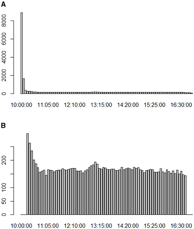
Figure 1. The graphs groups the sample by transaction time and counts missing data. (A) Here the sample is complete, from 10:00 to 16:55. (B) Here we have the filtered sample, from 10:15 to 16:40.

We sorted our database based on trading volume and selected the 50 most traded assets over the entire period. Despite continuous development, the Brazilian capital market still faces challenges related to liquidity. Liquidity issues become evident when working with the complete database, revealing anomalies in assets with very low trading volumes. Even with the application of interpolation or more advanced techniques to handle missing data, addressing low-liquidity assets proves to be problematic. The Table 1 shows a sector-wise overview of the assets in our sample.

Table 1

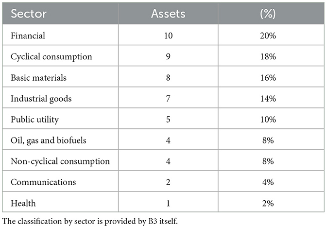
Table 1. Sample classified by economic sector.

Our sample excludes Exchange Traded Funds (ETF) BOVA11, which, despite being the fifth most traded asset in the period, would cause multicollinearity problems in our estimation. Despite filtering our database during the most critical times, a significant volume of missing data remains in the sample. To address this, we resort to interpolation methods. In our exercise, interpolation is performed in a univariate manner directly in the return series. The set of missing data in the sample is treated using smoothing cubic splines. We rely on the imputeTS library developed by Moritz and Bartz-Beielstein [50]. In other words, we fill in the missing data using cubic splines constructed with the asset's return series. Although there was an attempt to perform the filling via Kalman filter, the return series are filled with zeros, and when trying to interpolate the price series, we encountered convergence problems in executing the algorithm. Additionally, in terms of computational performance, we highlight the efficiency of filling via splines.

Interpolation by splines is an approach in which the interpolant is a particular type of piecewise polynomial called a spline. Instead of fitting a single high-degree polynomial to all values, we fit low-degree polynomials, in our case of degree 3, to small subsets of the values. This is a preferable method to polynomial interpolation because it helps reduce the interpolation error. Let x₁ < x₂ < ⋯ < x_n be the interpolation points. A cubic spline is a function s(x) defined on the interval [x₁, x_n] with the following properties:

• s(x), s′(x) and s″(x) are continuous functions on the interval (x₁, x_n).

• In each subinterval [x_i, x_i+1], s(x) is a cubic polynomial such that s(x_i) = f_i = f(x_i) for i = 1, dots, n.

Once the assets have been selected, the next step is to construct the daily covariance matrix. As discussed in the previous section, we chose to make the choice of matrix more flexible so that we can incorporate alternative methods and avoid using the sample covariance matrix. As an illustration, let's take naive example with two assets and two day that demonstrates the construction of the final dataset:

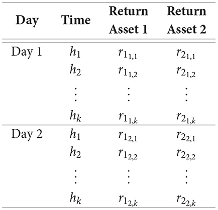
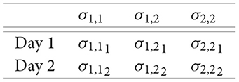
Here, h₁, …, h_k are the times of each trade. r_nt,k is the return on asset n, on day t and time k. This is our sample at the collection stage. Considering two assets, a covariance matrix Σ_t on day t will have the following format:

${\Sigma }_t=\left[\begin{array}{cc}{{\sigma }_{1,1}}_t& {{\sigma }_{1,2}}_t\\ {{\sigma }_{2,1}}_t& {{\sigma }_{2,2}}_t\end{array}\right]$

_σm,nt is the covariance between assets m and n, on day t. The intraday data is utilized to construct a daily proxy for the asset's volatility. We will consider vech(Σ_t) transposed so that we can have a row vector and additionally eliminate identical entries, given that it is a symmetric matrix. The algorithm works by excluding the lower triangle from the matrix. The data in its final version has the following configuration:

Generalizing to a sample of j days and n assets, our dataset will have j rows and n(n + 1)/2 columns. Finally, the data is all standardized, as required for the use of shrinkage methods Tibshirani et al. [34].

4.2 Estimation

In this work, we construct covariance matrices with daily frequency from the intraday data. The idea is for each component of the matrix to propose an estimation, equation by equation, such that a series of covariances or variances will be explained by their past and the past of all other elements in the matrix. To carry out the exercise, it is necessary to determine which covariance matrix will be calculated, as we pointed out in Section 3.

We compute the results for all the formats we present, in such a way that the proposed exercise consists of the following algorithm: for the return data, already filled in when missing, we calculate the daily covariance matrix, such that the final result is a dataset in which the columns are the elements of the matrix and the rows are the days of our sample. We separate 20% of the sample to construct a test set, and on the training basis, we estimate a model with 1 lag, that is, we write Σ_t as a function of Σ_t−1.

The estimation is done with the adaptation of glmnet, where the penalty criterion is chosen via the HQ information criterion. For each series, we estimate 11 models, such that each model has a value of α ∈ α_grid. Once the models are estimated, we construct the table with the modular loss function using out-of-sample data. This will be the data for running the MCS. Once this is done, we save the winning model based on the established significance level and choose the best model.

We chose to present the results in three formats:

• As in Medeiros et al. [30], our main reference, we calculate the selection of variables by sector, as depicted in the Figures 2A, 3A, 4A, 5A, 6A, 7A. This type of analysis allows us to identify effects within and between sectors. To simplify the axes of the graphs, the sectors will be denoted by their initials, i.e., CNC for non-cyclical consumption, BI for industrial goods, FIN for the financial sector, PGB for oil, gas, and biofuels, MB for basic materials, CC for cyclical consumption, UP for utility public, COM for communications, and SAU for health. The results are presented in a heatmap format, indicating the average percentage of shares selected by sector.

• To exemplify how to interpret the heatmap, let's use Figure 6A as an example: for Non-Cyclical Consumption (CNC), on average, 41% of the selected variances and covariances are from CNC, 7.7% are from Industrial Goods (BI), and so on. The rows represent the asset sector, and the columns show the average percentage of selected covariances. We also illustrate which models are eligible by economic sector to identify any patterns. The idea is to count and compute, by sector, which regressions are the winners within the MCS for each process. This information is presented in Figures 2B, 3B, 4B, 5B, 6B, 7B.

• Finally, we present the calculation of prediction errors. Traditional error measures are tabulated in Table 2. In the rows, we have the economic sector, and in the columns, the averages of the respective errors are displayed. The first column shows the mean of the Mean Absolute Error (MAE), the second shows the mean of the Mean Absolute Percentage Error (MAPE), the third shows the mean of the Mean Square Error (MSE), and finally, the fourth shows the mean of the Root Mean Square Error (RMSE).

Figure 2

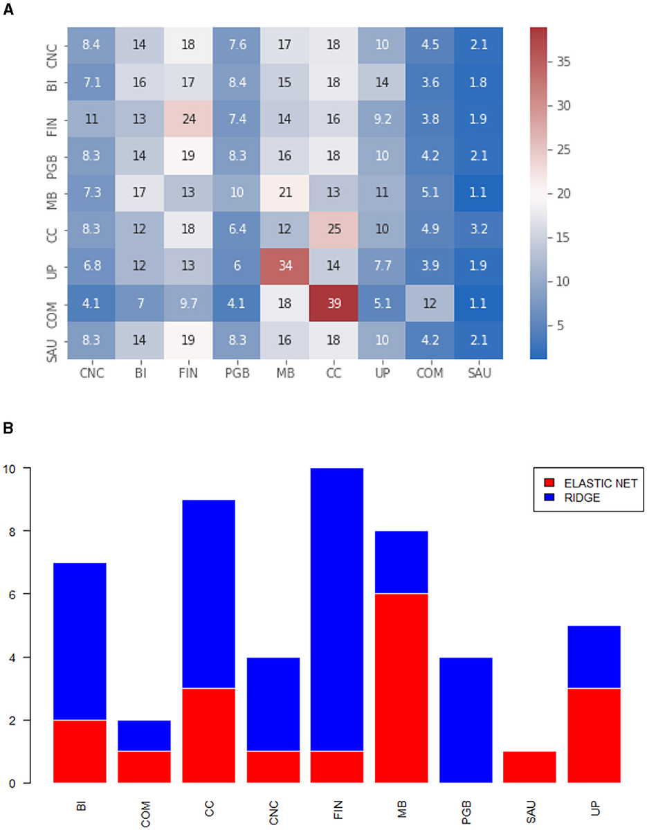
Figure 2. (A) Heatmap of the proportion of selected variables by economic sector. Diagonal elements. Matrix calculated via ewma. (B) Models selected by MCS, by economic sector. The numbers refer to the series that belong to the diagonal. Matrix calculated via ewma.

Figure 3

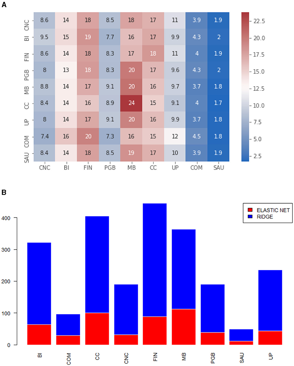
Figure 3. (A) Heatmap of the proportion of selected variables by economic sector. Off-diagonal elements. Matrix calculated via ewma. (B) Models selected by MCS, by economic sector. The numbers refer to the off-diagonal series. Matrix calculated via ewma.

Figure 4

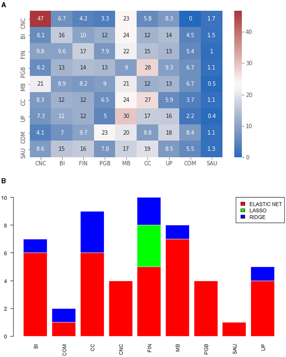
Figure 4. (A) Heatmap of the proportion of selected variables by economic sector. Diagonal elements. Matrix calculated via color. (B) Models selected by MCS, by economic sector. The numbers refer to the series that belong to the diagonal. Matrix calculated via color.

Figure 5

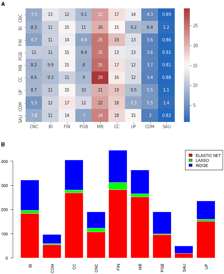
Figure 5. (A) Heatmap of the proportion of selected variables by economic sector. Off-diagonal elements. Matrix calculated via color. (B) Models selected by MCS, by economic sector. The numbers refer to the off-diagonal series. Matrix calculated via color.

Figure 6

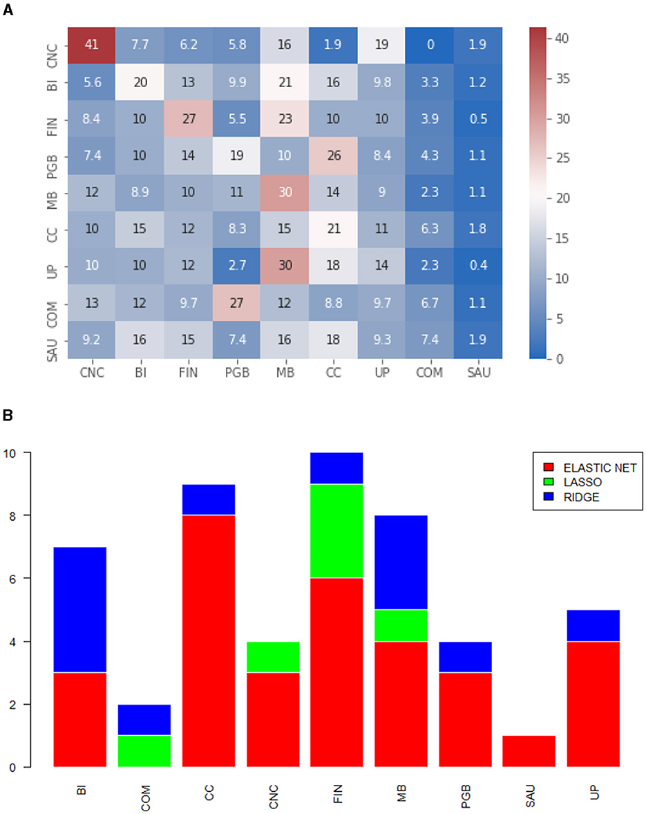
Figure 6. (A) Heatmap of the proportion of selected variables by economic sector. Diagonal elements. Matrix calculated via lw. (B) Models selected by MCS, by economic sector. The numbers refer to the series that belong to the diagonal. Matrix calculated via lw.

Figure 7

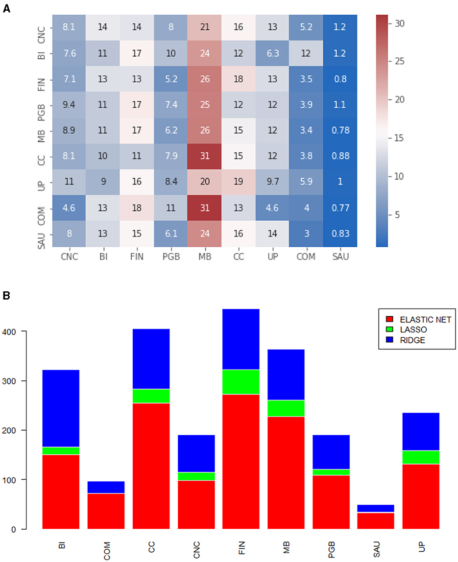
Figure 7. (A) Heatmap of the proportion of selected variables by economic sector. Off-diagonal elements. Matrix calculated via lw. (B) Models selected by MCS, by economic sector. The numbers refer to the off-diagonal series. Matrix calculated via lw.

Table 2

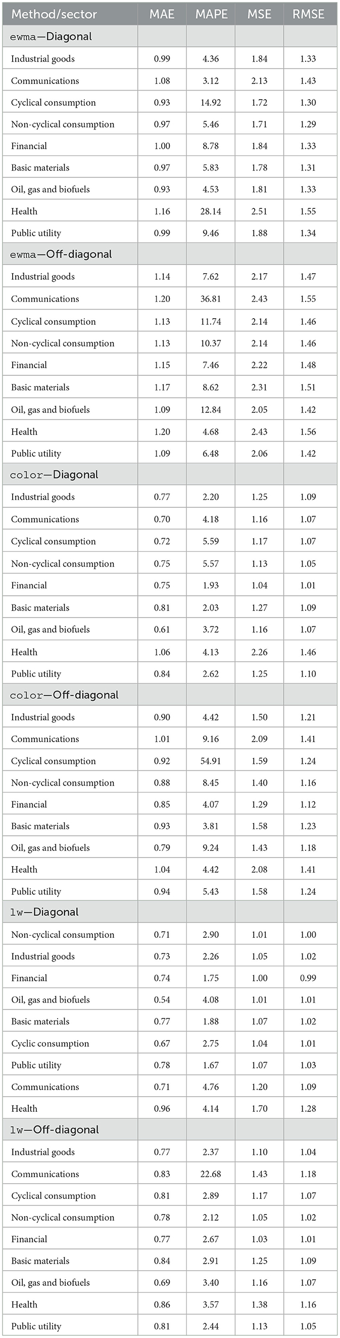
Table 2. Average of prediction errors for diagonal and off-diagonal elements my method and sector.

All results are presented from two perspectives: the elements within the main diagonal of the covariance matrix and the elements outside the diagonal. In other words, we separate the results into variances and covariances. An important observation to be made is the difficulty in classifying covariance between assets from different sectors. We decided to replicate our reference strategy and point out that the covariance process between an asset a and b belongs, mutually, to the economic sectors a and b, for a ≠ b.

4.2.1 Variance of type ewma

We observed from Figure 2A that there is not much pattern in the selected variables. We highlight the strong presence of the Basic Materials (MB) and Cyclical Consumption sectors. This result is consistent with the Brazilian market, which is not very liquid and highly correlated, as evident in the graph (Figure 2B). According to our algorithm, regression via LASSO was not chosen for any asset, comprising only Elastic Net and Ridge in the MCS. Due to the performance of Ridge regression in this matrix format, the proportion we see in the heatmap is close to the proportion we previously presented in Table 1. Convergent behavior was noticed for the off-diagonal elements. Figure 3A shows strong intensity in more liquid sectors, with emphasis on the Finance sector (FIN) and Basic Materials (MB). From the point of view of chosen models, we see almost equivalence between the graphs in Figures 2B, 3B. The off-diagonal elements did not present the LASSO regression for any process and mostly showed the choice of the Ridge-type regression.

4.2.2 Variance of type color

For this matrix format, we were also unable to detect clear patterns. We highlight the intra-sector effect of Non-Cyclical Consumption (CNC), with an average selection of 47%, of volatilities from the same sector. Basic Materials (MB) has a strong presence in almost all sectors and is involved in Public Utility (UP) volatilities. From a model selection point of view, this was the first matrix format that had LASSO regression chosen for some assets, but only for the financial sector. In the opposite direction of the matrix via ewma, we noticed a greater performance of the Elastic Net format. This is a more convergent result to the challenge of reducing dimension and does justice to the method of calculating the covariance matrix itself. For the covariance elements, off the diagonal, we note in Figure 5A a great predominance of Basic Materials (MB) and Cyclical Consumption (CC). From the Figure 5B, we have more gains in dealing with the size of the problem, as LASSO is computed in almost all sectors, except Health (SAU). If we compare the errors, we occasionally notice gains in predictive performance, as the results of the method color in Table 2 present better results compared to results of the method color in the same table.

4.2.3 Variance of type large

In this matrix format, we notice a clearer pattern within the diagonal processes. It is possible to observe in Figure 6A a greater intensity on the diagonal of the heatmap, indicating that the sector selects processes from the same sector more intensely, on average. This implies that the past of the volatility itself and the volatility of assets in the same sector are more relevant as features for a volatility process. Additionally, analyzing the model selection graph for the large format, we obtained greater gains compared to dimension reduction, as Ridge is the model that, among those eligible, is the least selected. Again, for the off-diagonal elements, we see a strong participation of the Basic Materials (MB) sector, as shown in Figure 7A. Covariances also benefit from more restrictive penalties, but we noticed Ridge regression across all sectors. From a predictive point of view, we have smaller measurements, on average, for this specific matrix format. This is, therefore, the type of covariance matrix estimation that generated the processes where the punctual estimation obtained better predictive performance and the ℓ₁ penalty was more effective, better facing the curse of dimensionality.

5 Conclusion

In this work, we study the realized volatility of Brazilian market data and analyze the predictive impact of choosing the covariance matrix. Using intraday trading data for 50 assets, daily covariance matrices were constructed. This approach allows the simultaneous computation of time-varying variances and covariances. Flexible covariance matrix methods enable the exercise to be conducted using alternative methods to sample covariance. The proposed estimation was autoregressive, aiming to identify how much the past of the series and the past of other processes influence a given covariance. Traditionally, via VAR, this exercise would entail specification and dimensionality problems due to the large number of covariates. Therefore, our proposal was based on a flexible algorithm that incorporates some shrinkage methodology, employing regressions with penalties.

Utilizing the Model Confidence Set algorithm proposed by Hansen et al. [10], we evaluated the predictive performance of the regressions and determined whether there is a statistically significant predictive gain in assigning Ridge, LASSO, or ElasticNet. The results obtained indicate that for challenges related to dimensionality and predictive gains, the outcome depends on how the covariance matrix is calculated. There is a direct relationship between the choice of variance or covariance processes and the liquidity of the corresponding sector.

As discussed in this study, the Brazilian market exhibits low liquidity, which limits the options available to investors in constructing trading strategies. Additionally, we found little relationship between distinct sectors: we demonstrated that, sectorally, what provides the most predictive gain for explaining volatilities are the volatilities of assets within the same sector. Alongside these findings, we also identified the financial sector as a relevant feature both within its own sector and across others: it is as if each economic sector possesses particular/idiosyncratic returns and volatility structures.

In the Brazilian financial market, the volatility of specific sectors has a considerable impact on the overall volatility of the stock exchange. Among these sectors, the financial sector stands out not only for its strategic importance but also for its significant impact on the dynamics of the stock market. The volatility of financial stocks often reflects not only the country's macroeconomic conditions but also sector-specific factors such as changes in regulatory policies, fluctuations in interest rates, and corporate events.

In periods of economic instability or political uncertainty, the volatility of financial sector stocks tends to increase, exerting additional pressure on the overall volatility of the Brazilian stock exchange. This is due to the significant weighting of financial companies in major market indices. As a result, investors and portfolio managers often closely monitor the volatility of these stocks as a key indicator of market sentiment and the degree of risk aversion. In the Brazilian stock market, the lack of strong correlation between economic sectors has significant implications for trading strategies, which have been the subject of study and analysis in academic financial literature. The absence of robust correlation suggests that price movements and the performance of one sector can occur independently of others, presenting both opportunities and challenges for traders [51].

On one hand, this low correlation allows traders to diversify their portfolios, capitalizing on performance variations between sectors and exploiting opportunities for gains in different market segments simultaneously [52]. Strategies focusing on sector arbitrage or dynamic asset allocation may be particularly effective in low sector correlation environments [53].

On the other hand, the lack of correlation also presents challenges as it makes it more difficult to identify consistent patterns or predict market movements based on traditional analyses [54]. Traders may struggle to develop robust forecasting models and anticipate the spread of shocks from one sector to another [55].

Therefore, traders operating in markets with low sector correlation often adopt more flexible and adaptive approaches, adjusting their strategies according to constantly changing market conditions [56]. Fundamental and technical analysis remains relevant, but the ability to adapt quickly to changes in market dynamics and identify emerging opportunities becomes crucial for trading success [57].

The work can be extended in several directions. An important extension is the inclusion of leverage effects [58] and conditional skewness [59–61] in the tested specifications. These effects are especially relevant in the analysis of intraday financial data, as discussed in Aït-Sahalia et al. [62] and Kambouroudis et al. [63]. Another very relevant extension is to analyze the impact of new information on the variance structure [64], using for example the news flow [65, 66] and market sentiments [67, 68] on the set of covariates for realized variance prediction.

Data availability statement

The data analyzed in this study is subject to the following licenses/restrictions. The datasets analyzed for this study are extracted from the B3 (Brasil, Bolsa e Balcão) exchange. Requests to access these datasets should be directed to laurini@fearp.usp.br.

Author contributions

LV: Conceptualization, Data curation, Formal analysis, Investigation, Methodology, Software, Writing – original draft, Writing – review & editing. ML: Conceptualization, Data curation, Investigation, Methodology, Writing – original draft, Writing – review & editing.

Funding

The author(s) declare financial support was received for the research, authorship, and/or publication of this article. The authors acknowledge funding from Capes, CNPq (310646/2021-9), and FAPESP (2023/02538-0).

Conflict of interest

The authors declare that the research was conducted in the absence of any commercial or financial relationships that could be construed as a potential conflict of interest.

Publisher's note

All claims expressed in this article are solely those of the authors and do not necessarily represent those of their affiliated organizations, or those of the publisher, the editors and the reviewers. Any product that may be evaluated in this article, or claim that may be made by its manufacturer, is not guaranteed or endorsed by the publisher.

Footnotes

1. ^Available at https://github.com/gabrielrvsc/HDeconometrics.

References

1. Andersen TG, Bollerslev T. Answering the skeptics: yes, standard volatility models do provide accurate forecasts. Int Econ Rev. (1998) 39:885–905. doi: 10.2307/2527343

Crossref Full Text | Google Scholar

2. Bollerslev T, Meddahi N, Nyawa S. High-dimensional multivariate realized volatility estimation. J Econom. (2019) 212:116–36. doi: 10.1016/j.jeconom.2019.04.023

Crossref Full Text | Google Scholar

3. Ledoit O, Wolf M. The power of (non-)linear shrinking: a review and guide to covariance matrix estimation. J Financial Econom. (2020) 20:187–218. doi: 10.1093/jjfinec/nbaa007

Crossref Full Text | Google Scholar

4. McAleer M, Medeiros MC. Realized volatility: a review. Econom Rev. (2008) 27:10–45. doi: 10.1080/07474930701853509

Crossref Full Text | Google Scholar

5. Sucarrat G. Identification of volatility proxies as expectations of squared financial returns. Int J Forecast. (2021) 37:1677–90. doi: 10.1016/j.ijforecast.2021.03.008

Crossref Full Text | Google Scholar

6. Laurini MP, Furlani LGC, Portugal MS. Empirical market microstructure: an analysis of the BRL/US$ exchange rate market. Emerg Mark Rev. (2008) 9:247–65. doi: 10.1016/j.ememar.2008.10.003

Crossref Full Text | Google Scholar

7. Yalaman A, Manahov V. Analysing emerging market returns with high-frequency data during the global financial crisis of 2007–2009. Eur J Finance. (2022) 28:1019–51. doi: 10.1080/1351847X.2021.1957698

Crossref Full Text | Google Scholar

8. Murphy KP. Machine Learning: A Probabilistic Perspective. Cambridge, MA: MIT Press (2013).

Google Scholar

9. Bühlmann P, van de Geer S. Statistics for High-Dimensional Data: Methods, Theory and Applications. Springer Series in Statistics. Heidelberg: Springer (2011). doi: 10.1007/978-3-642-20192-9

Crossref Full Text | Google Scholar

10. Hansen PR, Lunde A, Nason JM. The model confidence set. Econometrica. (2011) 79:453–97. doi: 10.3982/ECTA5771

Crossref Full Text | Google Scholar

11. Markowitz H. Portfolio selection*. J Finance. (1952) 7:77–91. doi: 10.1111/j.1540-6261.1952.tb01525.x

Crossref Full Text | Google Scholar

12. Bollerslev T. Generalized autoregressive conditional heteroskedasticity. J Econom. (1986) 31:307–27. doi: 10.1016/0304-4076(86)90063-1

Crossref Full Text | Google Scholar

13. Fleming J, Kirby C, Ostdiek B. The economic value of volatility timing using “realized” volatility. J Financ Econ. (2003) 67:473–509. doi: 10.1016/S0304-405X(02)00259-3

Crossref Full Text | Google Scholar

14. Engle RF. Autoregressive conditional heteroscedasticity with estimates of the variance of United Kingdom inflation. Econometrica. (1982) 50:987–1007. doi: 10.2307/1912773

Crossref Full Text | Google Scholar

15. Andersen TG, Davis RA, Kreiss JP, Mikosch T, Kreia JP, Kreiss JP. Handbook of Financial Time Series. Berlin: Springer (2016).

Google Scholar

16. Bollerslev T, Engle RF, Wooldridge JM. A capital asset pricing model with time-varying covariances. J Pol Econ. (1988) 96:116–31. doi: 10.1086/261527

Crossref Full Text | Google Scholar

17. Hansen PR, Lunde A. A forecast comparison of volatility models: does anything beat a Garch(1,1)? J Appl Econom. (2005) 20:873–89. doi: 10.1002/jae.800

Crossref Full Text | Google Scholar

18. Martin V, Hurn S, Harris D. Econometric Modelling with Time Series: Specification, Estimation and Testing. Themes in Modern Econometrics. Cambridge, MA: Cambridge University Press. (2012). doi: 10.1017/CBO9781139043205

Crossref Full Text | Google Scholar

19. Bauwens L, Laurent S, Rombouts JVK. Multivariate GARCH models: a survey. J Appl Econom. (2006) 21:79–109. doi: 10.1002/jae.842

Crossref Full Text | Google Scholar

20. Engle RF, Kroner KF. Multivariate simultaneous generalized arch. Econom Theory. (1995) 11:122–50. doi: 10.1017/S0266466600009063

Crossref Full Text | Google Scholar

21. Engle R. Dynamic conditional correlation: a simple class of multivariate generalized autoregressive conditional heteroskedasticity models. J Bus Econ Stat. (2002) 20:339–50. doi: 10.1198/073500102288618487

Crossref Full Text | Google Scholar

22. Engle R, Kelly B. Dynamic equicorrelation. J Bus Econ Stat. (2011) 30:212–28. doi: 10.1080/07350015.2011.652048

Crossref Full Text | Google Scholar

23. Barndorff-Nielsen OE, Shephard N. Econometric analysis of realized volatility and its use in estimating stochastic volatility models. J R Stat Soc B: Stat Methodol. (2002) 64:253–80. doi: 10.1111/1467-9868.00336

Crossref Full Text | Google Scholar

24. Andersen TG, Bollerslev T, Diebold FX, Labys P. Modeling and forecasting realized Volatility. Econometrica. (2003) 71:579–625. doi: 10.1111/1468-0262.00418

Crossref Full Text | Google Scholar

25. Hansen PR, Lunde A. Realized variance and market microstructure noise. J Bus Econ Stat. (2006) 24:127–61. doi: 10.1198/073500106000000071

Crossref Full Text | Google Scholar

26. Fan J, Fan Y, Lv J. High dimensional covariance matrix estimation using a factor model. J Econom. (2008) 147:186–97. doi: 10.1016/j.jeconom.2008.09.017

PubMed Abstract | Crossref Full Text | Google Scholar

27. Fan J, Liao Y, Mincheva M. High-dimensional covariance matrix estimation in approximate factor models. Ann Stat. (2011) 39:3320–56. doi: 10.1214/11-AOS944

PubMed Abstract | Crossref Full Text | Google Scholar

28. Fan J, Lv J, Qi L. Sparse high-dimensional models in economics. Annu Rev Econom. (2011) 3:291–317. doi: 10.1146/annurev-economics-061109-080451

PubMed Abstract | Crossref Full Text | Google Scholar

29. Fan J, Zhang J, Yu K. Vast portfolio selection with gross-exposure constraints. J Am Stat Assoc. (2012) 107:592–606. doi: 10.1080/01621459.2012.682825

PubMed Abstract | Crossref Full Text | Google Scholar

30. Medeiros M, Callot L, Kock A. Modeling and forecasting large realized covariance matrices and portfolio choice. J Appl Econom. (2017) 32:140–58. doi: 10.1002/jae.2512

Crossref Full Text | Google Scholar

31. Alves RP, de Brito DS, Medeiros MC, Ribeiro RM. Forecasting large realized covariance matrices: the benefits of factor models and shrinkage*. J Financ Econom. (2023) nbad013. doi: 10.1093/jjfinec/nbad013

Crossref Full Text | Google Scholar

32. Chamberlain G, Rothschild M. Arbitrage, factor structure, and mean-variance analysis on large asset markets. Econometrica. (1983) 51:1281–304. doi: 10.2307/1912275

Crossref Full Text | Google Scholar

33. Ledoit O, Wolf M. Honey, I shrunk the sample covariance matrix. J Portfolio Manag. (2004) 30:110–9. doi: 10.3905/jpm.2004.110

Crossref Full Text | Google Scholar

34. Tibshirani R, Hastie T, Wainwright M. Statistical Learning with Sparsity: The Lasso and Generalizations. Boca Raton, FL: Chapman & Hall/CRC. (2015).

Google Scholar

35. Laurini MP, Ohashi A. A noisy principal component analysis for forward rate curves. Eur J Oper Res. (2015) 246:140–53. doi: 10.1016/j.ejor.2015.04.038

Crossref Full Text | Google Scholar

36. Tibshirani R, Hastie T, Friedman J. The Elements of Statistical Learning. Springer Series in Statistics. New York, NY: Springer New York Inc. (2001).

Google Scholar

37. Jobson JD, Korkie B. Estimation for Markowitz efficient portfolios. J Am Stat Assoc. (1980) 75:544–54. doi: 10.1080/01621459.1980.10477507

Crossref Full Text | Google Scholar

38. Michaud RO. The Markowitz optimization enigma: is ‘optimized' optimal? Financ Anal J. (1989) 45:31–42. doi: 10.2469/faj.v45.n1.31

Crossref Full Text | Google Scholar

39. Fan J, Liao Y, Liu H. An overview of the estimation of large covariance and precision matrices. Econom J. (2016) 19:C1–C32. doi: 10.1111/ectj.12061

Crossref Full Text | Google Scholar

40. Ardia D, Boudt K, Gagnon-Fleury JP. RiskPortfolios: computation of risk-based portfolios in R. J Open Source Softw. (2017) 2:171. doi: 10.21105/joss.00171

Crossref Full Text | Google Scholar

41. Morgan JP. RiskMetrics: Technical Document. New Yok, NY: Reuters Ltd International Marketing Martin Spencer (1996).

Google Scholar

42. Ledoit O, Wolf M. A well-conditioned estimator for large-dimensional covariance matrices. J Multivar Anal. (2004) 88:365–411. doi: 10.1016/S0047-259X(03)00096-4

Crossref Full Text | Google Scholar

43. Friedman J, Hastie T, Tibshirani R. Regularization paths for generalized linear models via coordinate descent. J Stat Softw. (2010) 33:1–22. doi: 10.18637/jss.v033.i01

PubMed Abstract | Crossref Full Text | Google Scholar

44. Hoerl AE, Kennard RW. Ridge regression: biased estimation for nonorthogonal problems. Technometrics. (2000) 42:80–6. doi: 10.1080/00401706.2000.10485983

Crossref Full Text | Google Scholar

45. Tibshirani R. Regression shrinkage and selection via the Lasso. J R Stat Soc B. (1996) 58:267–88. doi: 10.1111/j.2517-6161.1996.tb02080.x

Crossref Full Text | Google Scholar

46. Zou H, Hastie T. Regularization and variable selection via the elastic net. J R Stat Soc B. (2005) 67:301–20. doi: 10.1111/j.1467-9868.2005.00503.x

Crossref Full Text | Google Scholar

47. Hamilton JD. Time Series Analysis. Princeton, NJ: Princeton University Press. (1994). doi: 10.1515/9780691218632

Crossref Full Text | Google Scholar

48. Bernardi M, Catania L. The model confidence set package for R. Innov Finance Account EJournal. (2014) 1–20. doi: 10.2139/ssrn.2692118

Crossref Full Text | Google Scholar

49. Perlin M, Ramos H. GetHFData: a R package for downloading and aggregating high frequency trading data from Bovespa. Rev Bras Finanças. (2016) 14:443–78.

Google Scholar

50. Moritz S, Bartz-Beielstein T. imputeTS: time series missing value imputation in R. R J. (2017) 9:207–18. doi: 10.32614/RJ-2017-009

Crossref Full Text | Google Scholar

51. Narayan SW, Rehman MU, Ren YS, Ma C. Is a correlation-based investment strategy beneficial for long-term international portfolio investors? Financ Innov. (2023) 9:64. doi: 10.1186/s40854-023-00471-9

PubMed Abstract | Crossref Full Text | Google Scholar

52. Buraschi A, Porchia P, Trojani F. Correlation risk and optimal portfolio choice. J Finance. (2010) 65:393–420. doi: 10.1111/j.1540-6261.2009.01533.x

Crossref Full Text | Google Scholar

53. Burgess N. An Introduction to Arbitrage Trading Strategies (April 16, 2023). Available online at: https://ssrn.com/abstract=4420232

Google Scholar

54. Kritzman M, Page S, Turkington D. In defense of optimization: the fallacy of 1/n. Financ Anal J. (2012) 68:31–9. doi: 10.2469/faj.v68.n3.3

Crossref Full Text | Google Scholar

55. Boudt K, Daníelsson J, Laurent S. Robust forecasting of dynamic conditional correlation GARCH models. Int J Forecast. (2013) 29:244–57. doi: 10.1016/j.ijforecast.2012.06.003

Crossref Full Text | Google Scholar

56. Hidaka R, Hamakawa Y, Nakayama J, Tatsumura K. Correlation-diversified portfolio construction by finding maximum independent set in large-scale market graph. IEEE Access. (2023) 11:142979–91. doi: 10.1109/ACCESS.2023.3341422

Crossref Full Text | Google Scholar

57. Greig AC. Fundamental analysis and subsequent stock returns. J Account Econ. (1992) 15:413–42. doi: 10.1016/0165-4101(92)90026-X

Crossref Full Text | Google Scholar

58. Christie A. The stochastic behavior of common stock variances: value, leverage and interest rate effects. J Financ Econ. (1982) 10:407–32. doi: 10.1016/0304-405X(82)90018-6

Crossref Full Text | Google Scholar

59. Engle RF, Gonzalez Rivera G. Semiparametric ARCH models. J Bus Econ Stat. (1991) 9:345–59. doi: 10.1080/07350015.1991.10509863

Crossref Full Text | Google Scholar

60. De Luca G, Loperfido N. A Skew-in-mean Garch model for financial returns. In: Genton MG, , editor. Skew-Elliptical Distributions and Their Applications: A Journey Beyond Normality. Boca Raton, FL: CRC/Chapman & Hall (2004). p. 205–22. doi: 10.1201/9780203492000.ch12

Crossref Full Text | Google Scholar

61. De Luca G, Genton MG, Loperfido N. A multivariate Skew-Garch model. In: Terrell D, , editor. Advances in Econometrics: Econometric Analysis of Economic and Financial Time Series, Part A, Vol. 20. Oxford: Elsevier (2006). p. 33–56. doi: 10.1016/S0731-9053(05)20002-6

Crossref Full Text | Google Scholar

62. Aït-Sahalia Y, Fan J, Li Y. The leverage effect puzzle: disentangling sources of bias at high frequency. J Financ Econ. (2013) 109:224–49. doi: 10.1016/j.jfineco.2013.02.018

Crossref Full Text | Google Scholar

63. Kambouroudis DS, McMillan DG, Tsakou K. Forecasting realized volatility: the role of implied volatility, leverage effect, overnight returns, and volatility of realized volatility. J Futures Mark. (2021) 41:1618–39. doi: 10.1002/fut.22241

Crossref Full Text | Google Scholar

64. Cutler DM, Poterba JM, Summers LH. What moves stock prices? J Portfolio Manag. (1989) 15:4–12. doi: 10.3905/jpm.1989.409212

Crossref Full Text | Google Scholar

65. Darolles S, Gouriéroux C, Fol GL. Intraday transaction price dynamics. Ann Econ Stat. (2000) 60:207–38. doi: 10.2307/20076261

Crossref Full Text | Google Scholar

66. Seok S, Cho H, Ryu D. Scheduled macroeconomic news announcements and intraday market sentiment. N Am J Econ Finance. (2022) 62:101739. doi: 10.1016/j.najef.2022.101739

Crossref Full Text | Google Scholar

67. Gao B, Liu X. Intraday sentiment and market returns. Int Rev Econ Finance. (2020) 69:48–62. doi: 10.1016/j.iref.2020.03.010

Crossref Full Text | Google Scholar

68. Seok SI, Cho H, Ryu D. Stock Market's responses to intraday investor sentiment. N Am J Econ Finance. (2021) 58:101516. doi: 10.1016/j.najef.2021.101516

Crossref Full Text | Google Scholar