Analytical solutions of the space–time fractional Kadomtsev–Petviashvili equation using the (G’/G)-expansion method

1 Introduction

Nonlinear partial differential equation (NPDEs) play a crucial role in characterizing an array of phenomena across diverse fields. For example, in the field of physics, numerous issues such as fluid mechanics, nonlinear dynamics, plasma physics, and wave motions can be described through NPDEs. Furthermore, NPDE applications span across various fields such as engineering, mechanics, and chemistry; as mentioned in Dodd et al. (1). Gaining a comprehensive understanding of these nonlinear phenomena can be achieved by finding exact solutions for NPDEs. As a result, several approaches have been developed to accurately solve NPDEs using precise numerical techniques, such as the Backlund transformation and the Homotopy perturbation method, and others (2–7). Moreover, numerous potent techniques have been recently developed, such as the (G′/G)-expansion method and others (8–12).

Kadomtsev and Petviashvili (13) introduced a nonlinear equation as an extension of the well-known Kortewe de-Vries (KdV) equation. The mathematical representation of the Kadomtsev and Petviashvili (KP) equation is

$\begin{array}{ll}{\left(U_t+aU{U}_x+b{U}_{xxx}\right)}_x+\gamma U_{yy}=0,& (1)\end{array}$

where $a$ and $b$ are constant, the function $U\left(x,y,t\right)$ represents spatial directions $x$ and $y$, along with time $t$, and $\gamma$ is a constant scalar which can be either ±1. Based on Eq. (1), when $a=b=1$, the space–time fractional Kadomtsev–Petviashvili (FKP) equation is given as follows:

$\begin{array}{ll}{D}_{tx}^{\alpha \alpha }U+D_x^{\alpha }{U}^2+U\mathrm{\hspace{0.33em}}{D}_x^{\alpha \alpha }U+D_x^{\alpha \alpha \alpha \alpha }U+\gamma D_y^{\alpha \alpha }U=0.& (2)\end{array}$

This paper focusses on finding exact wave solutions of Eq. (2) by employing the conformable fractional derivative (CFD). The CFD, initially introduced by Khalil et al. (14), is a revolutionary step in the realm of fractional calculus, with the derivative showcasing essential qualities that have broad implications across a myriad of disciplines, including but not limited to the domains of mathematics, engineering, and physics. Within Eq. (2), we denote the CFD in reference to time $\left(t\right)$ and space $\left(x\right)$ using $D_t^{\alpha }$ and $D_x^{\alpha }$, accordingly. Moreover, we define higher-order operations such as $D_x^{\alpha \alpha }U=D_x^{\alpha }\left(D_x^{\alpha }U\right)$ for the second-order and $D_x^{\alpha \alpha \alpha \alpha }U=D_x^{\alpha }\left(D_x^{\alpha \alpha \alpha }\right)$ for the fourth-order CFDs. The use of CFD within soliton theory is primarily advantageous due to its capacity for effectively characterizing soliton wave behaviors and providing profound physical insights. With these merits in mind, this paper applies the (G’/G)-expansion method to derive traveling wave solutions for Eq. (2) setting $\gamma =1$. The paper builds upon existing scholarly interest in fractional dimensions as observed in the FKP equation and supported by literature references (15, 16), among references therein.

The (G’/G)-expansion method, presented by Wang et al. (9), is widely used to construct traveling wave solutions of different NPDEs. However, its application to the FKP equation remains relatively unexplored. Consequently, the novelty of this research lies in the application of the (G’/G)-expansion method to the FKP equation as this method has not been widely applied to this particular equation. Numerous studies have previously utilized this method in the examination of different NPDEs to extract traveling wave solutions, as illustrated in references (17–22). Recognizing the limitations of current solution methods for the FKP equation, the motivation of this paper is to harness the power of the (G’/G)-expansion method to unearth analytical solutions. This not only promises to expand the repository of exact solutions available for the FKP equation but also stands to offer deeper insights into the complex behaviors of fractional-order nonlinear systems. The main objective of this paper is to study the use of (G’/G)-expansion method in order to find analytical solutions to the FKP equation and to explore the implications of these solutions for understanding the behavior of nonlinear systems. By utilizing traveling wave transformation, the FKP equation was transformed into an ordinary differential equation (ODE), leading to discover more comprehensive exact analytical solutions. Consequently, a more comprehensive range of exact analytical solutions for the FKP equation was obtained. Graphical illustrations are included to elucidate the physical characteristics of the acquired solutions. To demonstrate the impact of the fractional operator on results, the acquired solutions are exhibited for different values of the fractional order α, with a comparison to their corresponding exact solutions when taking the conventional scenario where α equals 1. The structure of this article is as follows: Section 2 covers the conformable fractional derivative. In section 3, the (G’/G)-expansion method is described in detail. In section 4, solutions for the space–time FKP equation are presented. Section 5 showcases graphical representations to illustrate the physical characteristics of the derived solutions. Finally, the paper concludes with section 6.

2 Materials and methods

This section introduces the fundamental review of the CFD, G’/G-expansion method and its application.

2.1 Conformable fractional derivative

In this subsection, we present a concise discussion of the fundamental properties of CFD, following the monographs authored by Khalil et al. (14). We define the conformable derivative of order α, where 0 < α ≤ 1, with respect to the independent variable $x$ as

$\begin{array}{l}{D}^{\alpha }U\left(x\right)=\underset{\epsilon \to 0}{\lim }\frac{U\left(x+\epsilon x^{1-\alpha }\right)-U\left(x\right)}{\epsilon },\\ x>0,\alpha \in \left(0,1\right],U^{\alpha }\left(0\right)=\underset{t\to 0^{+}}{\lim }{D}^{\alpha }U\left(x\right).\end{array}\text{ (3)}$

This well-formed fractional derivative is obtained by adhering to certain essential properties. Let us consider the derivative order $\alpha \in \left(0,1\right]$, and suppose that for all positive values of $x$, $U$ and $V$ represent $\alpha$-differentiable functions with $a$ and $b$ as constants. Using Eq. (3), we obtain the following properties:

• $D^{\alpha }{x}^{\tau }=\tau x^{\tau -\alpha },\tau \in ℝ.$

• $D^{\alpha }a=0.$

• $D^{\alpha }U\left(x\right)=x^{1-\alpha }\mathrm{\hspace{0.33em}}\frac{dU}{dx}.$

• $D^{\alpha }\left(aU+bV\right)=a{D}^{\alpha }U+b{D}^{\alpha }V.$

• $D^{\alpha }\left(UV\right)=U{D}^{\alpha }V+V{D}^{\alpha }U.$

• $D^{\alpha }\left(\frac{U}{V}\right)=\frac{V{D}^{\alpha }U-U{D}^{\alpha }V}{V^2}.$

• $D^{\alpha }\left(U\left(V\left(x\right)\right)\right)=\frac{dU}{dV}{D}^{\alpha }V\left(x\right)=x^{1-\alpha }\mathrm{\hspace{0.33em}}\frac{dU}{dV}\frac{dV}{dx}.$

These properties have been well proven and share many properties with integer derivatives (14, 23). It is noted that the conformable differential operator complies with several fundamental principles analogous to those of the chain rule, Taylor series expansion, and Laplace transformation (24). In this paper, the FKP equation is translated into an ODE within the context of CFD.

2.2 Description of the (G’/G)-expansion method

In what follow, we highlight the key steps of the G’/G-expansion method:

Step 1: We assume that the nonlinear fractional partial differential equation including $x,y$ and $t$ as follows:

$\begin{array}{ll}P\left(U,D_t^{\alpha }U,D_x^{\alpha }U,D_y^{\alpha }U,D_t^{\alpha \alpha }U,D_t^{\alpha }\left(D_x^{\alpha }U\right),D_x^{\alpha \alpha }U,D_y^{\alpha \alpha }U\dots \right)=0,& (4)\end{array}$

where $U\left(x,y,t\right)$ is the result of this equation.

Step 2: Solutions of Eq. (4) are obtained by considering the following traveling wave transformation

$\begin{array}{ll}U\left(x,y,t\right)=u\left(\xi \right),\xi =\xi \left(x,y,t\right).& (5)\end{array}$

By substituting Eq. (5) into Eq. (4), the ODE is obtained as follows:

$\begin{array}{ll}P\left(u,u^{\prime },u^{″},u^{‴},\cdots \right)=0,& (6)\end{array}$

where the superscript is expressed as the derivative concerning $\xi$.

Step 3: Solutions of Eq. (6) are represented as

$\begin{array}{ll}u\left(\xi \right)={{\displaystyle \sum }}_{i=-m}^m{\rho }_i{\left(\frac{G^{\prime }}{G}\right)}^i,& (7)\end{array}$

where ${\rho }_i$ remains constant, $m$ designates a positive integer whose value will be determined and the function $G=G\left(\xi \right)$ fulfills a second order ODE in the form

$\begin{array}{ll}{G}^{″}+\lambda G^{\prime }+\mu G=0,& (8)\end{array}$

where $\lambda$ and $\mu$ are constants. Depending on the sign of $\left({\lambda }^2-4\mu \right)$, Eq. (6) has a family of solutions as:

$\text{Family}1:\text{For}{\lambda }^2-4\mu >0,$

$\frac{G^{\prime }\left(\xi \right)}{G\left(\xi \right)}=\frac{\sqrt{{\lambda }^2-4\mu }}{2}\left[\frac{\begin{array}{l}A\sinh \left(\frac{1}{2}\sqrt{{\lambda }^2-4\mu }\xi \right)\\ +B\cosh \left(\frac{1}{2}\sqrt{{\lambda }^2-4\mu }\xi \right)\end{array}}{\begin{array}{l}A\cosh \left(\frac{1}{2}\sqrt{{\lambda }^2-4\mu }\xi \right)\\ +B\sinh \left(\frac{1}{2}\sqrt{{\lambda }^2-4\mu }\xi \right)\end{array}}\right]-\frac{\lambda }{2}.\text{ (9)}$

Case 1: when $A\ne 0,B=0$, in Eq. (9), we get

$\begin{array}{ll}\frac{G^{\prime }\left(\xi \right)}{G\left(\xi \right)}=\frac{\sqrt{{\lambda }^2-4\mu }}{2}\tanh \left(\frac{1}{2}\sqrt{{\lambda }^2-4\mu }\xi \right)-\frac{\lambda }{2}.& (10)\end{array}$

Case 2: when $A=0,B\ne 0$, we have

$\begin{array}{ll}\frac{G^{\prime }\left(\xi \right)}{G\left(\xi \right)}=\frac{\sqrt{{\lambda }^2-4\mu }}{2}\coth \left(\frac{1}{2}\sqrt{{\lambda }^2-4\mu }\xi \right)-\frac{\lambda }{2}.& (11)\end{array}$

$\text{Family}2:\text{For}{\lambda }^2-4\mu <0,$

$\frac{G^{\prime }\left(\xi \right)}{G\left(\xi \right)}=\frac{\sqrt{{\lambda }^2-4\mu }}{2}\left[\frac{\begin{array}{l}A\cos \left(\frac{1}{2}\sqrt{{\lambda }^2-4\mu }\xi \right)\\ -B\sin \left(\frac{1}{2}\sqrt{{\lambda }^2-4\mu }\xi \right)\end{array}}{\begin{array}{l}A\sin \left(\frac{1}{2}\sqrt{{\lambda }^2-4\mu }\xi \right)\\ +B\cos \left(\frac{1}{2}\sqrt{{\lambda }^2-4\mu }\xi \right)\end{array}}\right]-\frac{\lambda }{2}.\text{ (12)}$

Case 1: when $A\ne 0,B=0$, in Eq. (12), we obtain

$\begin{array}{ll}\frac{G^{\prime }\left(\xi \right)}{G\left(\xi \right)}=\frac{\sqrt{{\lambda }^2-4\mu }}{2}\cot \left(\frac{1}{2}\sqrt{{\lambda }^2-4\mu }\xi \right)-\frac{\lambda }{2}.& (13)\end{array}$

Case 2: when $A=0,B\ne 0$, we have

$\begin{array}{ll}\frac{G^{\prime }\left(\xi \right)}{G\left(\xi \right)}=-\frac{\sqrt{{\lambda }^2-4\mu }}{2}\tan \left(\frac{1}{2}\sqrt{{\lambda }^2-4\mu }\xi \right)-\frac{\lambda .}{2}& (14)\end{array}$

$\text{Family}3:\text{For}{\lambda }^2-4\mu =0,$

Case 1: when $A=1,B=1$, we get

$\begin{array}{ll}\frac{G^{\prime }\left(\xi \right)}{G\left(\xi \right)}=\frac{1}{1+\xi }-\frac{\lambda }{2}.& (15)\end{array}$

2.3 Application

In this subsection, the G’/G-expansion method is utilized to derive wave solutions for Eq. (2) when $\gamma =1$. This case transforms Eq. (2) as follows:

$\begin{array}{ll}{D}_{tx}^{\alpha \alpha }U+D_x^{\alpha }{U}^2+U\mathrm{\hspace{0.33em}}{D}_x^{\alpha \alpha }U+D_x^{\alpha \alpha \alpha \alpha }U+D_y^{\alpha \alpha }U=0.& (16)\end{array}$

Now, consider the following traveling wave transformation

$\begin{array}{ll}U\left(x,y,t\right)=u\left(\xi \right),\zeta =\frac{1}{\alpha }\left(x^{\alpha }+\sigma y^{\alpha }-c{t}^{\alpha }\right).& (17)\end{array}$

Taking Eq. (17) into Eq. (16), Eq. (16) converts to an ODE, and integrating the resultant equation twice, we get

$\begin{array}{ll}\left({\sigma }^2-c\right)\mathrm{\hspace{0.33em}}u+\frac{1}{2}{u}^2+u^{″}=0,& (18)\end{array}$

where $\sigma$ and $c$ are constants. By equating the nonlinear term $u^2$ to the highest derivative $u^{″}$, we determine that $m=2$. Thus, Eq. (7) becomes

$\begin{array}{ll}u\left(\xi \right)={\rho }_{-2}{\left(\frac{G^{\prime }}{G}\right)}^{-2}+{\rho }_{-1}{\left(\frac{G^{\prime }}{G}\right)}^{-1}+{\rho }_0+{\rho }_1\left(\frac{G^{\prime }}{G}\right)+{\rho }_2{\left(\frac{G^{\prime }}{G}\right)}^2.& (19)\end{array}$

Substituting Eq. (19) into Eq. (18), we obtain

$\begin{array}{l}\beta \left(\begin{array}{l}{\rho }_{-2}{\left(\frac{G^{\prime }}{G}\right)}^{-2}+{\rho }_{-1}{\left(\frac{G^{\prime }}{G}\right)}^{-1}\\ +{\rho }_0+{\rho }_1\left(\frac{G^{\prime }}{G}\right)+{\rho }_2{\left(\frac{G^{\prime }}{G}\right)}^2\end{array}\right)+\frac{1}{2}{\left(\begin{array}{l}{\rho }_{-2}{\left(\frac{G^{\prime }}{G}\right)}^{-2}+{\rho }_{-1}{\left(\frac{G^{\prime }}{G}\right)}^{-1}\\ +{\rho }_0+{\rho }_1\left(\frac{G^{\prime }}{G}\right)+{\rho }_2{\left(\frac{G^{\prime }}{G}\right)}^2\end{array}\right)}^2\\ +{\left({\rho }_{-2}{\left(\frac{G^{\prime }}{G}\right)}^{-2}+{\rho }_{-1}{\left(\frac{G^{\prime }}{G}\right)}^{-1}+{\rho }_0+{\rho }_1\left(\frac{G^{\prime }}{G}\right)+{\rho }_2{\left(\frac{G^{\prime }}{G}\right)}^2\right)}^{\prime \prime }=0,\end{array}\text{ (20)}$

$\text{where\hspace{1em}\hspace{1em}}\beta ={\sigma }^2-c.$

Substituting Eq. (8) into Eq. (20) and methodically collecting all terms by corresponding powers of G’/G, we establish a coherent set of algebraic equations through the equating of each term’s coefficient to zero within Eq. (20). These algebraic equations are then resolved utilizing the computational capabilities of Maple to obtain the following

$\text{Set}1:\begin{array}{c}\mu =-\frac{1}{16}\beta ,{\rho }_0=-\frac{1}{2}\beta ,\lambda =0,\\ {\rho }_1=0,{\rho }_2=-12,{\rho }_{-2}=-\frac{3}{64}{\beta }^2,{\rho }_{-1}=0.\end{array}\}\text{ (21)}$

$\text{Set}2:\begin{array}{c}\mu =\frac{1}{16}\beta ,{\rho }_0=-\frac{3}{2}\beta ,\lambda =0,\\ {\rho }_1=0,{\rho }_2=-12,{\rho }_{-2}=-\frac{3}{64}{\beta }^2,{\rho }_{-1}=0.\end{array}\}\text{ (22)}$

$\text{Set}3:\begin{array}{c}\mu =-\frac{1}{4}\beta +\frac{1}{4}{\lambda }^2,{\rho }_0=-3{\lambda }^2+\beta ,\lambda =\lambda ,\\ {\rho }_1=0,{\rho }_2=0,{\rho }_{-2}=-\frac{3}{4}{\left(\beta -{\lambda }^2\right)}^2,{\rho }_{-1}=3\left(\beta -{\lambda }^2\right)\lambda .\end{array}\}\text{ (23)}$

$\text{Set}4:\begin{array}{c}\mu =\frac{1}{4}\beta +\frac{1}{4}{\lambda }^2,{\rho }_0=-3{\lambda }^2-3\beta ,\lambda =\lambda ,\\ {\rho }_1=0,{\rho }_2=0,{\rho }_{-2}=-\frac{3}{4}{\left(\beta +{\lambda }^2\right)}^2,{\rho }_{-1}=-3\left(\beta +{\lambda }^2\right)\lambda .\end{array}\}\text{ (24)}$

$\text{Set}5:\begin{array}{c}\mu =\frac{1}{4}\beta +\frac{1}{576}{\rho }_1^2,{\rho }_0=-\frac{1}{48}{\rho }_1^2-3\beta ,\lambda =-\frac{1}{12}{\rho }_1,\\ {\rho }_1={\rho }_1,{\rho }_2=-12,{\rho }_{-2}=0,{\rho }_{-1}=0.\end{array}\}\text{ (25)}$

$\text{Set}6:\begin{array}{c}\mu =-\frac{1}{4}\beta +\frac{1}{576}{\rho }_1^2,{\rho }_0=-\frac{1}{48}{\rho }_1^2+\beta ,\lambda =-\frac{1}{12}{\rho }_1,\\ {\rho }_1={\rho }_1,{\rho }_2=-12,{\rho }_{-2}=0,{\rho }_{-1}=0.\end{array}\}\text{ (26)}$

$\text{Set}7:\begin{array}{c}\mu =\lambda =0,{\rho }_0=-2\beta \\ {\rho }_1=0,{\rho }_2=0,{\rho }_{-2}=0,{\rho }_{-1}=0.\end{array}\}\text{ (27)}$

We finally get the exact solutions of Eq. (16), where the solutions are derived according to the following:

Family 1:

In case 1, substituting Eq. (21) into Eq. (10) yields

$\begin{array}{l}{U}_1\left(x,y,t\right)=-\frac{1}{2}\left({\sigma }^2-c\right)[1+\frac{3}{2}{\tanh }^2\left(\frac{\sqrt{{\sigma }^2-c}}{4\alpha }\left(x^{\alpha }+\sigma y^{\alpha }-c{t}^{\alpha }\right)\right)\\ +\frac{3}{2}{\coth }^2\frac{\sqrt{{\sigma }^2-c}}{4\alpha }\left(x^{\alpha }+\sigma y^{\alpha }-c{t}^{\alpha }\right)];{\sigma }^2>c.\end{array}\text{ (28)}$

In case 1, substituting Eq. (26) into Eq. (10) introduces

$\begin{array}{l}{U}_2\left(x,y,t\right)\\ =\left({\sigma }^2-c\right)[1-3{\tanh }^2\left(\frac{\sqrt{{\sigma }^2-c}}{4\alpha }\left(x^{\alpha }+\sigma y^{\alpha }-c{t}^{\alpha }\right)\right)];{\sigma }^2>c.\end{array}\text{ (29)}$

In case 2, substituting Eq. (23) into Eq. (11) gives

$\begin{array}{l}{U}_3\left(x,y,t\right)=\left({\sigma }^2-c-3{\lambda }^2\right)+3\left({\sigma }^2-c-{\lambda }^2\right)\\ (\frac{\sqrt{{\sigma }^2-c}}{2\lambda }\coth \left(\frac{\sqrt{{\sigma }^2-c}}{2\alpha }\left(x^{\alpha }+\sigma y^{\alpha }-c{t}^{\alpha }\right)\right)-{\frac{1}{2}}^{-1}\\ -\frac{\left({\sigma }^2-c-{\lambda }^2\right)}{4}\\ \frac{\sqrt{{\sigma }^2-c}}{2}\coth \left(\frac{\sqrt{{\sigma }^2-c}}{2\alpha }\left(x^{\alpha }+\sigma y^{\alpha }-c{t}^{\alpha }\right)\right)-{\frac{\lambda }{2}}^{-2});{\sigma }^2>c.\end{array}\text{\hspace{1em}\hspace{1em}\hspace{1em}\hspace{1em}\hspace{0.5em}\hspace{1em} (30)}$

Family 2:

In case 1, substituting Eq. (22) into Eq. (13) gives

$\begin{array}{l}{U}_4\left(x,y,t)\right)=\frac{3}{2}\left(c-{\sigma }^2\right)[1-\frac{1}{2}{\cot }^2\left(\frac{\sqrt{c-{\sigma }^2}}{4\alpha }\left(x^{\alpha }+\sigma y^{\alpha }-c{t}^{\alpha }\right)\right)\\ -\frac{1}{2}{\tan }^2\frac{\sqrt{c-{\sigma }^2}}{4\alpha }\left(x^{\alpha }+\sigma y^{\alpha }-c{t}^{\alpha }\right)];{\sigma }^2<c.\end{array}\text{ (31)}$

In case 1, substituting Eq. (25) into Eq. (13) yields

$\begin{array}{l}{U}_5\left(x,y,t)\right)=-3\left({\sigma }^2-c\right)[1-{\cot }^2\left(\frac{\sqrt{c-{\sigma }^2}}{4\alpha }\left(x^{\alpha }+\sigma y^{\alpha }-c{t}^{\alpha }\right)\right)];\\ {\sigma }^2<c.\end{array}\text{ (32)}$

In case 2, substituting Eq. (24) into Eq. (14) presents

$\begin{array}{l}{U}_6\left(x,y,t\right)=-3\left({\sigma }^2-c+{\lambda }^2\right)\\ (1-\frac{\sqrt{c-{\sigma }^2}}{2\lambda }\tan \left(\frac{\sqrt{c-{\sigma }^2}}{2\alpha }\left(x^{\alpha }+\sigma y^{\alpha }-c{t}^{\alpha }\right)\right)+{\frac{1}{2}}^{-1}\\ +\frac{\left({\sigma }^2-c+{\lambda }^2\right)}{4}\frac{\sqrt{c-{\sigma }^2}}{2}\tan \left(\frac{\sqrt{c-{\sigma }^2}}{2\alpha }\left(x^{\alpha }+\sigma y^{\alpha }-c{t}^{\alpha }\right)\right)+{\frac{\lambda }{2}}^{-2});\\ {\sigma }^2<c.\end{array}\text{ (33)}$

Family 3:

In this case, substituting Eq. (27) into Eq. (15) provides

$\begin{array}{ll}{U}_7\left(x,y,t\right)=\frac{1}{1+\left(\frac{1}{\alpha }\left(x^{\alpha }+\sigma y^{\alpha }-c{t}^{\alpha }\right)\right)};{\sigma }^2=c.& (34)\end{array}$

3 Graphical representations of the obtained solutions

In what follow, we delineate three-dimensional (3D) graphical depictions which portray the acquired solutions at assorted space and time intervals, with different values of the fractional order parameter α.

The 3D graphs in Figure 1 depicts the nonlinear soliton solutions of $U_1\left(x,y,t\right)$ characterized by parameters $c=1,\sigma =2,y=2$ and within the range $0\le x,t\le 10$ as per Eq. (28), elucidating the dynamics of non-linear wave propagation. The depiction embraces the exact solutions of $U_1\left(x,y,t\right)$ for fractional orders $\alpha =1,\alpha =0.98,\alpha =0.96$ and $\alpha =0.94$, offering kink soliton solutions with absolute values delineated in Figures 1A–D accordingly. It is noteworthy within Figure 1 that an increase in the value of $\alpha$ is inversely related to the magnitude of $U_1\left(x,y,t\right)$. For comprehensiveness, it is paramount to articulate that same behavior are exhibited by nonlinear waves within solutions $U_4\left(x,y,t\right),U_6\left(x,y,t\right)$ and $U_7\left(x,y,t\right)$, as witnessed in their respective 3D representations akin to those demonstrated for $U_1\left(x,y,t\right).$

Figure 1

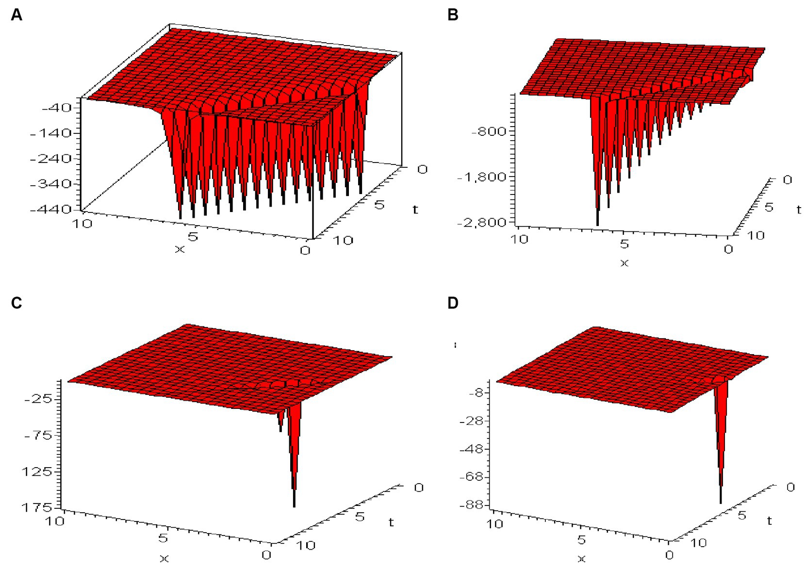
Figure 1. 3D graph of solutions $U_1\left(x,y,t\right)forc=1$, $\sigma =2$, $y=2with$ $0\le x,t\le 10.$.

In exploring the dynamic features of nonlinear wave propagation as delineated in Eq. (30) and Figure 2 illustrates the 3D graphical depictions of the wave solutions for $U_3\left(x,y,t\right)$, constructed under parameters set at $c=1,\sigma =2,\lambda =1$ and $y=2$ over a domain where $0\le x,t\le 10$. Noteworthy within these illustrations is the depiction of solitary wave solutions at different $\alpha$ values—specifically $\alpha =1,\alpha =0.98,\alpha =0.96$ and $\alpha =0.94$ corresponding individually to Figure 2A–D. A clear pattern that emerges from Figure 2 is the direct relationship between $\alpha$ values and the resultant wavelength; an increment in $\alpha$ is associated with an increase in the wavelength. Concurrently, a diminutive trend in amplitude is noted as $\alpha$ decreases from 1 to 0.94.

Figure 2

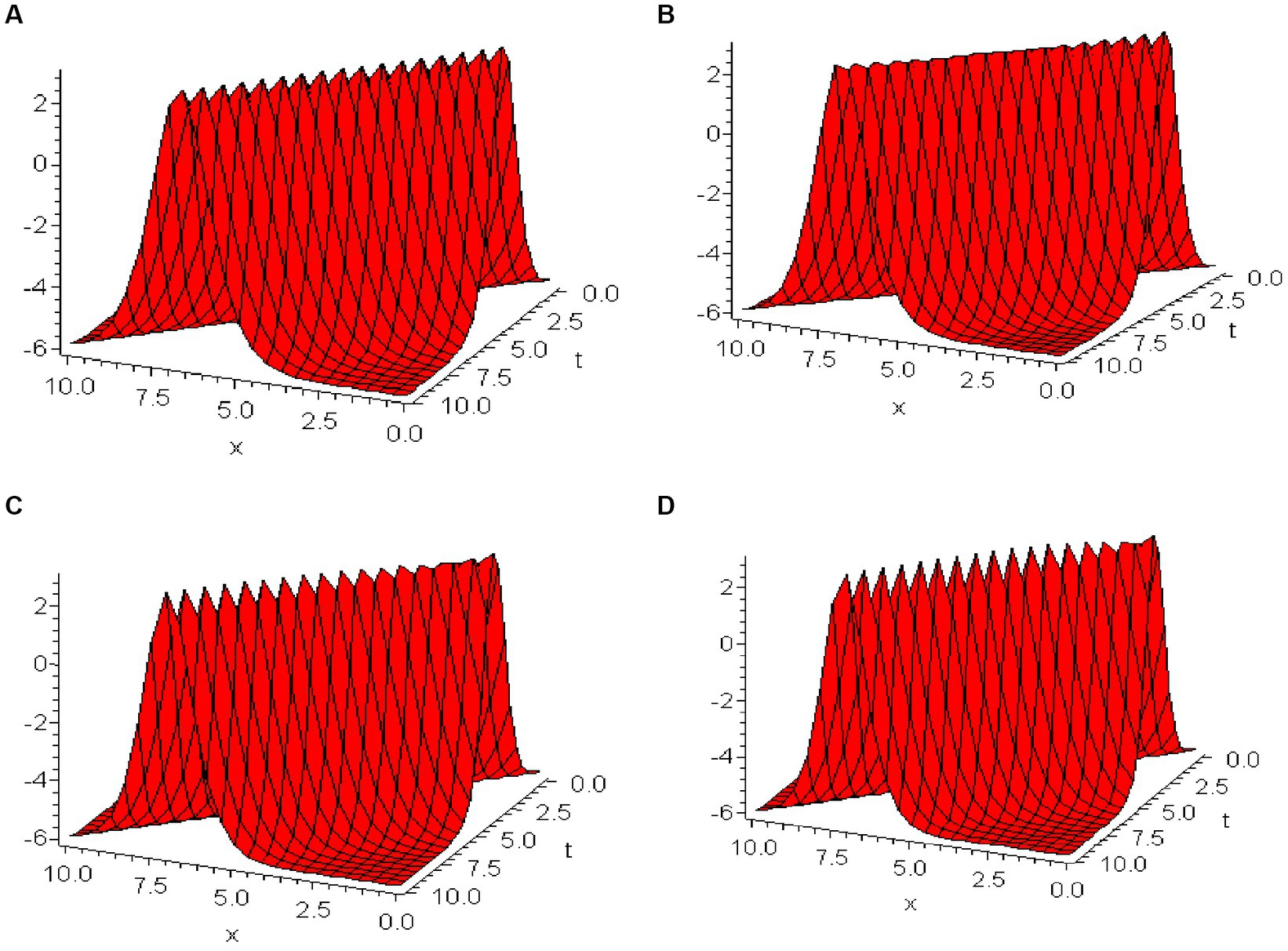
Figure 2. 3D graph of solutions $U_3\left(x,y,t\right)forc=1$, $\sigma =2$, $y=2,=1with$ $0\le x,t\le 10.$.

Figure 3 displays the 3D graphical representations of the solution $U_5\left(x,y,t\right)$, under specified conditions: $c=1,\sigma =2,\lambda =1$ and $y=2$. The value range for both $x$ and $t$ is restricted between 0 and 10. The values of $\alpha$ are set at 1, 0.98, 0.96, and 0.94 for Figures 3A–D, respectively. These graphs are crucial in illustrating the kink soliton solutions that arise from the nonlinear wave dynamics as governed by Eq. (32). Notably, a diminution in the value of $\alpha$ correlates with the propagation of the wavefront toward higher values on the $x$-axis.

Figure 3

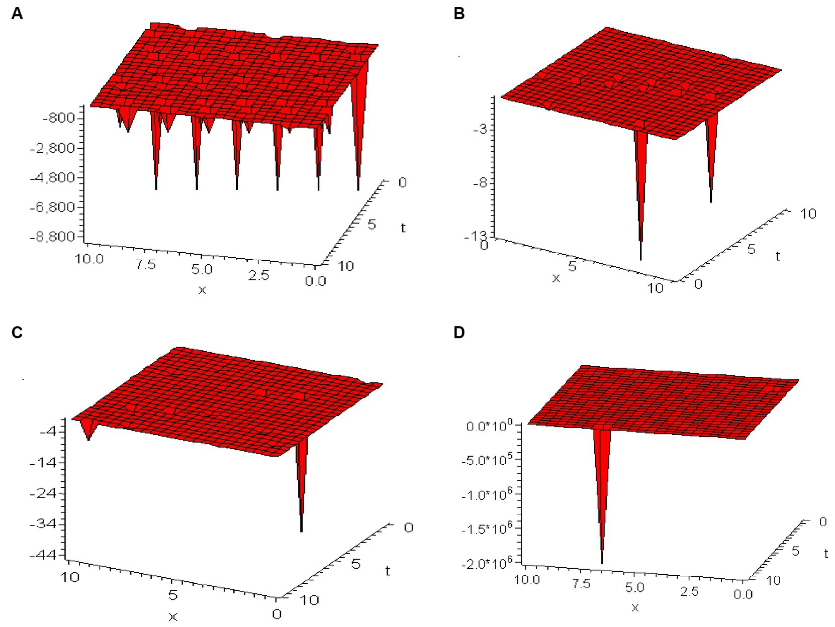
Figure 3. 3D graph of solution $U_5\left(x,y,t\right)forc=4$, $\sigma =1$, $y=2,=1with$ $0\le x,t\le 10.$.

4 Conclusion

In this paper, the (G’/G)-expansion method has been efficiently utilized to obtain analytical solutions for the fractional Kadomtsev–Petviashvili (FKP) equation involving the conformable fractional derivative (CFD). A range of exact analytical solutions for the FKP equation has been obtained. To demonstrate the impact of the fractional operator on results, the acquired solutions are exhibited for different values of the fractional order α, with a comparison to their corresponding exact solutions when taking the conventional scenario where α equals 1. This has been done to discern the impact of varying fractional-orders α to delineate how variations in α influence the properties of the solutions. The physical characteristics of the acquired solutions have been illustrated through various graphical representations. The results of this paper demonstrates the potency, simplicity, and efficacy of the (G’/G)-expansion approach. This method holds potential for tackling numerous challenges across diverse disciplines. Ultimately, the derived results can hold significant value for computational and experimental investigations in wave studies. All calculations within this study were conducted using MAPLE. Further research could be undertaken to study the numerical solutions of the FKP equation as well as analytical solutions of the stochastic FKP equation.

Data availability statement

The original contributions presented in the study are included in the article/supplementary material, further inquiries can be directed to the corresponding author.

Author contributions

AH: Writing – review & editing. MS: Writing – review & editing. Gk: Writing – original draft. EG: Writing – original draft. AA: Writing – original draft. AS: Writing – original draft.

Funding

The author(s) declare that no financial support was received for the research, authorship, and/or publication of this article.

Acknowledgments

The authors extend their appreciation to the Deanship of Scientific Research at Northern Border University, Arar, KSA for funding this research work through the project number “NBU-FFR-2024-1266-01.”

Conflict of interest

The authors declare that the research was conducted in the absence of any commercial or financial relationships that could be construed as a potential conflict of interest.

Publisher’s note

All claims expressed in this article are solely those of the authors and do not necessarily represent those of their affiliated organizations, or those of the publisher, the editors and the reviewers. Any product that may be evaluated in this article, or claim that may be made by its manufacturer, is not guaranteed or endorsed by the publisher.

References

1. Dodd, RK, Eilbeck, JC, Gibbon, JD, and Morris, HC. Solitons and nonlinear wave equations. New York, NY, USA: Academic Press (1982).

Google Scholar

2. Rogers, C, and Shadwick, WF. Bäcklund transformations and their applications. New York, NY, USA: Academic Press (1982).

Google Scholar

3. Hirota, R. Exact solution of the Korteweg-de Vries equation for multiple collisions of solitons. Phys Rev Lett. (1971) 27:1192–4. doi: 10.1103/PhysRevLett.27.1192

Crossref Full Text | Google Scholar

4. Gardner, CS, Greene, JM, Kruskal, MD, and Miura, RM. Method for solving the Korteweg-deVries equation. Phys Rev Lett. (1967) 19:1095–7. doi: 10.1103/PhysRevLett.19.1095

Crossref Full Text | Google Scholar

5. Adomian, G. Solving frontier problems of physics: The decomposition method. New York, NY, USA: Springer (1993).

Google Scholar

6. He, JH. Variational iteration method for delay differential equations. Commun Nonlinear Sci Numer Simul. (1997) 2:235–6. doi: 10.1016/S1007-5704(97)90008-3

Crossref Full Text | Google Scholar

7. He, JH. Homotopy perturbation technique. Comp Meth Appl Mech and Engine. (1999) 178:257–62. doi: 10.1016/S0045-7825(99)00018-3

Crossref Full Text | Google Scholar

8. Abdou, MA. The extended tanh-method and its applications for solving nonlinear physical models. Appl Math Comput. (2007) 190:988–96. doi: 10.1016/j.amc.2007.01.070

Crossref Full Text | Google Scholar

9. Wang, M, Li, X, and Zhang, J. The (G’/G)-expansion method and travelling wave solutions of nonlinear evolution equations in mathematical physics. Phys Lett A. (2008) 372:417–23. doi: 10.1016/j.physleta.2007.07.051

Crossref Full Text | Google Scholar

10. Wang, Z, and Zhang, HQ. A new generalized riccati equation rational expansion method to a class of nonlinear evolution equation with nonlinear terms of any order. Appl Math Comput. (2007) 186:693–704. doi: 10.1016/j.amc.2006.08.015

Crossref Full Text | Google Scholar

11. Gepreel, KA. Analytical methods for nonlinear evolution equations in mathematical physics. Mathematics. (2020) 8:2211. doi: 10.3390/math8122211

Crossref Full Text | Google Scholar

12. Zhang, S. A generalized auxiliary equation method and its application to (2+1)-dimensional Kortewegáde Vries equations. Comput Math Appl. (2007) 54:1028–38. doi: 10.1016/j.camwa.2006.12.046

Crossref Full Text | Google Scholar

13. Kadomtsev, BB, and Petviashvili, VI. On the stability of solitary waves in weakly dispersive media. Sov Phys Dokl. (1970) 15:539–41.

Google Scholar

14. Khalil, R, Horani, MA, Yousef, A, and Sababhehb, M. A new definition of fractional derivative. J Comput Appl Math. (2014) 264:65–70. doi: 10.1016/j.cam.2014.01.002

Crossref Full Text | Google Scholar

15. Linares, F, Pilod, D, and Saut, J-C. The Cauchy problem for the fractional Kadomtsev--Petviashvili equations. SIAM J Math Anal. (2018) 50:3172–209. doi: 10.1137/17M1145379

Crossref Full Text | Google Scholar

16. Pava, JA. Stability properties of solitary waves for fractional KdV and BBM equations. Nonlinearity. (2018) 31:920–56. doi: 10.1088/1361-6544/aa99a2

Crossref Full Text | Google Scholar

17. Feng, J, Li, W, and Wan, Q. Using (G′/G)-expansion method to seek traveling wave solution of Kolmogorov-Petrovskii-Piskunov equation. Appl Math Comput. (2011) 217:5860–5. doi: 10.1016/j.amc.2010.12.071

Crossref Full Text | Google Scholar

18. Naher, H, Abdullah, F, and Akbar, M. The (G′/G)-expansion method for abundant traveling wave solutions of caudrey-dodd-gibbon equation. Math Probl Eng. (2011) 2011:1–11. doi: 10.1155/2011/218216

Crossref Full Text | Google Scholar

19. Abazari, R, and Abazari, R. Hyperbolic, trigonometric and rational function solutions of Hirota-Ramanie equation via (G′/G)-expansion method. Math Probl Eng. (2011) 2011:1–11. doi: 10.1155/2011/424801

Crossref Full Text | Google Scholar

20. Zayed, EME. Traveling wave solutions for higher dimensional nonlinear evolution equations using the (G′/G)-expansion method. J Appl Maths Inform. (2010) 28:383–95. doi: 10.1155/2011/424801

Crossref Full Text | Google Scholar

21. Jabbari, A, Kheiri, H, and Bekir, A. Exact solutions of the coupled higgs equation and the miccari system using He’s semi-inverse method and (G′/G)-expansion method. Comput Math Appl. (2011) 62:2177–86. doi: 10.1016/j.camwa.2011.07.003

Crossref Full Text | Google Scholar

22. Ozis, T, and Aslan, I. Application of the (G′/G)-expansion method to kawahara type equations using symbolic computation. Appl Math Comput. (2010) 216:2360–5. doi: 10.1016/j.amc.2010.03.081

Crossref Full Text | Google Scholar

23. Biragni, OT, Chandok, S, Dedovic, N, and Radenovic, S. A note on some recent results of the conformable derivative. Adv Theory Nonlin Analy Appl. (2019) 3:11–7. doi: 10.31197/atnaa.482525

Crossref Full Text | Google Scholar

24. Abdeljawad, T. On conformable fractional calculus. J Comput Appl Math. (2015) 279:57–66. doi: 10.1016/j.cam.2014.10.016

Crossref Full Text | Google Scholar