The application of propensity score methods in observational studies

1 Introduction

In observational studies, such as in social public affairs, the formulation or assertion of various decisions requires robust evidence to support them. Analyzing the effects of decisions involves examining the relationships between variables, commonly using methods such as linear regression and logistic regression. However, real-world data often exhibit complex relationships, with variables potentially showing quadratic or even more intricate correlations. Additionally, due to various reasons, measurement errors might exist in the data, and linear models are heavily influenced by outliers. In such cases, linear models may not accurately describe the relationships between variables and may struggle to effectively address selection bias, thus impacting the accuracy of causal inference. The adoption of an inappropriate model could lead to decision errors and significant losses. Therefore, it is necessary to explore different methods, such as Propensity Score (PS) based methods—Propensity Score Matching (PSM), Inverse Probability Weighting (IPW) and Augmented IPW (AIPW), and conduct comprehensive comparative analyses to ensure reliable results. In this article, we apply PS methods to analyze datasets from three different fields: scientific research, natural biology, and demography. We discuss the advantages of PS methods over methods such as linear regression and introduce interaction terms in the linear regression model to provide partial corroboration for the results obtained from the analysis using PS methods.

In the study on the influence of research papers, Uzzi et al. [1] conclude that papers exhibiting both high conventionality and novelty are more likely to become hit papers. We replicate their experiment on the DBLP dataset and grouped the papers based on their novelty and conventionality to calculate the probability of becoming hit papers. Papers scoring high in both novelty and conventionality showed a 2.9 times higher probability of becoming hit papers compared to those with low scores in both aspects. However, when incorporating other confounding variables and using PS methods to calculate the probability ratio, the results were all smaller compared to the original conclusion. So relying solely on the ratio of probabilities may lead to a biased estimation of the quality of the papers. Similarly, when reviewing funding proposals, experts who assess projects solely based on their novelty and conventionality may make erroneous judgments and this will lead to the misallocation of resources toward relatively low-output and low-efficiency directions.

The study conducted by Vollaard and van Ours [2] on the fairness of herring ratings reveals that in the regression analysis of herring scores concerning whether they are supplied by Atlantic, the coefficientfor for Atlantic is significant at the 5% confidence level. Therefore, they concluded there was a bias in favor of Atlantic in the ratings. Vollaard's findings have had a significant impact on the reputation of Atlantic, leading to substantial economic losses and raising public concerns regarding the fairness of the ratings. However, according to all three PS analyses, after controlling for other variables related to herring, it can not be concluded that herring supplied by Atlantic receives significantly higher scores compared to others. Thus, we can not assert bias in the ratings. Through a more appropriate linear regression analysis, the coefficient for Atlantic is also found to be non-significant, providing further confirmation of this result.

In the study on how education influences health, Cheng et al. [3] verified that education can have a positive impact on the physical health of the elderly through influencing health behaviors and socioeconomic factors. In their analysis, the former has a greater effect. However, according to other three PS analyses, when only controlling for leisure index, one variable in the health behavior category, the coefficient for education is no longer significant, indicating that we cannot definitively claim that education has a significant impact on health. Furthermore, when controlling for variables related to diet, the coefficient for education decreases compared to the baseline model, suggesting that education may not have an impact on health through this specific channel. Therefore, in health education, it may be more effective to focus on leisure activities rather than promoting healthy eating, or increasing financial subsidies for the elderly.

In this paper, we employ PS methods to estimate the treatment effects and provide supplementary analysis to the original conclusions. PS methods achieve an approximation of a randomized experiment by weighting or matching samples based on their propensity scores. The paper is structured as follows, in Section 2 we introduce the PS methods, while in Sections 3–5 we present the analyses of the DBLP dataset, the herring dataset, and the CLHLS dataset, respectively. In Section 6 we conduct simulations to compare the estimation of treatment effects using various methods under different scenarios. In the final section we summarize the conclusion.

2 PS methods

Let Z represents different experimental exposure, where Z = 1 if sample is assigned to treatment group and Z = 0 otherwise. The outcomes when samples are assigned to control and treatment groups are denoted as (Y(0), Y(1)). But for a specified individual only one of (Y(0), Y(1)) can be observed; hence, they are usually referred to as potential outcomes. In observational studies, there is often an issue of selection bias—(Y(0), Y(1)) are not independent of the group assignment variable Z. In this situation, the distribution of confounding variables differs between the two groups, and these confounding variables may also influence potential outcomes. Consequently, the difference between the average observed responses of the two groups contains both the effect of the treatment and confounding variables. Comparing the difference in average observed responses directly to estimate the treatment effect may lead to errors.

For example, if we want to calculate the average treatment effect ATE = E(Y(1) − Y(0)). This represents the difference in the expected outcomes of the sample assigned to treatment and control group. The average response of the treatment group, i.e., E(Y(1)|Z = 1), is not equal to E(Y(1)) due to confounding variables. In order to estimate ATE more accurately, various methods such as linear regression, PSM, IPW and AIPW can be used for analysis.

Let X denote confounding variables. When calculating treatment effects, VanderWeele [4] suggest selecting all variables that occur before the experiment. If the conditional independence assumption holds, i.e.,

$(Y(0),Y(1))╨Z|X,$

then we can conclude that E(Y(0)|Z = 0, X) = E(Y(0)|Z = 1, X). Hence we can select samples with the same values of the confounding variable and use the average outcomes of the control group as a substitute for E(Y(0)|Z = 1, X). However, as the dimension of the confounding variables increases, it becomes infeasible to select samples with the same values of the confounding variable. The PS methods [5–7] can address this issue. Propensity score refers to the probability of a sample receiving treatment given the confounding variables, denoted as e(X) = p(Z = 1|X) < 0 < e(X) < 1. Under the assumption of conditional independence, it can be proven that (Y(0), Y(1)) ╨ Z|e(X) holds, which means that we can describe the sample's propensity for the treatment solely based on the propensity score without considering all the confounding variables.

Intuitively, if two samples have similar propensity scores but receive different experimental treatments, it can be assumed that the potential outcomes for these samples are identified. This provides the possibility to estimate the treatment effect. To better utilize the samples, they can be divided into K strata Q₁, ..., Q_k, and the PSM estimator is

$\begin{array}{r}{\Delta }_{psm}={\displaystyle \sum _{j=1}^K\frac{n_j}{n}}\{n_{1j}^{-1}{\displaystyle \sum _{i=1}^n{Z}_i}{Y}_{i}1(e(X_i)\in Q_j)\\ -n_{0j}^{-1}{\displaystyle \sum _{i=1}^n(1-Z_i)}{Y}_{i}1(e(X_i)\in Q_j)\},\end{array}$

where n_kj is the number of samples belonging to both group Z = k and strata Q_j, moreover, $n_j=\sum _k{n}_{kj}$ and $n=\sum _j{n}_j$.

In applications, the number of strata in PSM method needs to be finely adjusted. Insufficient samples in certain strata can limit the effectiveness of matching. The idea behind IPW is to assign weights to the samples based on their propensity scores, aiming to make the distribution of confounding variables more similar between two groups [8]. This decouples the influence of treatment and confounding variables on the outcomes, so the difference in outcomes is only due to different experimental exposures, making it analogous to the scenario of randomized experiment. Taking the calculation of ATE as an example. When estimating E(Y(0)), we assign weights w(X) to samples in control group, ensuring that the distribution of confounding variables between the two groups is similar, i.e.

$w(X)\propto \frac{f(X)}{f(Z=0|X)}=\frac{1}{1-e(X)},$

It means that if the propensity score of sample in control group is higher, the probability of it receiving treatment is also higher, and the confounding variable distribution of it is more similar to the treatment group. By increasing the weight of samples in the control group with higher propensity scores and decreasing the weight of samples with lower propensity scores, the distributions of confounding variables for the two groups of samples can be made more similar. The estimated value of E(Y(0)) is $Ê(Y_0)=\frac{1}{n}{\displaystyle \sum _{i=1}^n}(1-Z_i)Y_i/(1-e(X_i))$, where C means control group and EY(1) can be obtained in a similar manner. Finally, the IPW estimator of ATE is

${\Delta }_{ipw}=\frac{1}{n}{\displaystyle \sum _{i=1}^n}\frac{Z_i{Y}_i}{e(X_i)}-\frac{1}{n}{\displaystyle \sum _{i=1}^n}\frac{(1-Z_i)Y_i}{1-e(X_i)}$

The IPW estimator highly depends on the accuracy of the propensity score. To address this issue, Robins et al. [9] proposed AIPW method, which includes the outcome model m_k(X) = E(Y|Z = k, X). When at least one of the outcome model and the propensity score model is accurate, the estimation of the treatment effect is accurate. Taking ATE as an example, the AIPW estimator is

$\begin{array}{l}{\Delta }_{aipw}=\frac{1}{n}{\displaystyle \sum _{i=1}^n}(\frac{Z_i{Y}_i}{e(X_i)}-\frac{Z_i-e(X_i)}{e(X_i)}{m}_1(X_i))\\ -\frac{1}{n}{\displaystyle \sum _{i=1}^n}(\frac{(1-Z_i)Y_i}{1-e(X_i)}+\frac{Z_i-e(X_i)}{1-e(X_i)}{m}_0(X_i)).\end{array}$

Furthermore, the asymptotic variance of the AIPW estimator is smaller than that of the IPW estimator [9].

PS method uses tree-based models to estimate the propensity score. It splits the data into different subtrees by selecting a splitting point each time. The complexity of the model can be controlled by limiting the tree's depth and the number of samples in each leaf node. This method bypasses the linear assumption and uses non-parametric functions for classification. Moreover, tree-based models automatically select variables and are less sensitive to outliers.

However, when using tree models for analysis, we typically can only use the Bootstrap method to compute the variance or standard error (SE) of the estimates. In contrast, the estimation of variance in linear regression is relatively straightforward, but the assumption of linear relationship does not always hold true. Introducing a large number of cross-term features may cause overfitting issues, particularly in situations with limited data.

The propensity score method divides the estimation of treatment effects into two steps: the first step involves using the estimated propensity scores for weighting or matching, and the second step entails the estimation of effects based on the simulated random experiment scenarios. In practical applications, we assume that the estimation of the propensity scores is accurate and evaluate the treatment effects using t-test based solely on the results of the first step, thereby avoiding the time-consuming Bootstrap method.

PS methods are widely applied in various fields such as healthcare and social sciences. Li et al. [10] utilized IPW method to adjust the weights of the samples, making the distribution of women's confounding variables—age, BMI, and others similar between the treatment and control groups. They conclude that there is no significant reduction in the probability of developing pregnancy-induced hypertension by taking a certain nutrient during early pregnancy. Thomas et al. [11] employed IPW method to analyze the relationship between food security and children health. They find that children from households with food security issues are more likely to delay treatment due to financial constraints. These children are also more likely to have difficulty affording healthcare, dental care, and mental health services. Additionally, they are more prone to experiencing chronic symptoms such as asthma, skin allergies, and depression. Besides, while their acute illness symptoms are similar to those of other children, they are more susceptible to colds and gastrointestinal problems in the past two weeks. PS methods have also been widely applied in other studies [12, 13].

3 DBLP dataset

Uzzi et al. [1] conducted an in-depth study on the importance of novelty and conventionality in determining the impact of scientific papers. Their research revealed a significant phenomenon in scientific research and provided insights and profound understanding of scientific development. They analyzed the Web of Science (WOS) dataset and measured the novelty and conventionality of paper citations by examining the citation counts in reference combinations. The findings show that papers with high level of conventionality and novelty has a probability of 9.11% of becoming hit papers, while papers with low levels of both have a probability of 2.05% of becoming hit papers. Thus, they conclude that papers with high novelty and conventionality are more likely to become hit papers.

Uzzi et al. combined referenced papers in pairs and recorded their citations counts received in the year of publication. For computational feasibility, they used journal combinations to replace paper combinations. They then standardized these citation counts based on the observed citation counts of the same combinations in randomized citation networks. To create the randomized citation networks, they randomly selected two papers and two references published in the same year respectively, exchanged their citation relationships, and repeated this process multiple times. They repeated this procedure to generate 10 random citation networks and recorded the citation counts for each journal combination. The normalized citation count for each journal combination was calculated as the z-score, which describes the rarity or commonness of the frequency with which the references are cited together compared to the random networks. For a given paper, the z-score values of all journal combinations formed by its references were computed. The high novelty of a paper was defined as having 10th-percentile below zero, while the high conventionality of a paper was defined as having a median z-score value higher than the median z-score value of all journal combinations.

Because WOS dataset is not publicly available, we conduct our analysis on the DBLP-Citation-network V12 [14] dataset (DBLP), which yield similar results to the original study. We select papers published between 1965 and 2015 and define hit paper as one ranking in the top 5% of citations within a 5-year period. The DBLP dataset contains 4.89 million papers and 45.56 million citation records. Using the aforementioned method, we calculate the conventional and novel characteristics for each paper. The results show that the probability of papers with both high conventional and novel characteristics becoming hit papers is 8.6%, while the probability for papers with low scores in both characteristics is 2.9%. Papers with high scores in both characteristics are 2.94 times more likely to become hit papers compared to papers with low scores in both characteristics, which is roughly consistent with the results from the WOS dataset.

Assuming Z = 1 indicates both high novelty and conventionality of the paper, and Z = 0 indicates both are low, then the assessment of the impact of novelty and conventionality on the paper requires the estimation of

$RR=\frac{EY(1)}{EY(0)}.$

In the analysis by Uzzi et al., they did not consider other confounding variables that could influence citation counts, such as the number of citations the author has received in the past which represents the author's academic impact. The distribution of confounding variables is different between the two groups of papers, so the estimation of the probability ratio of becoming a hit paper E(Y(1)|Z = 1)/E(Y(0)|Z = 0) includes the effects of confounding variables, novelty and conventionality, and this may lead to biased estimates.

We rigorously select variables occurring before the paper under analysis, including the number of hit papers published by the corresponding author in the past 5–10 years (hit_cnt_corr_5yrs), the number of papers published by the first author in the past 3 and 5 years (pub_cnt_fir_3yrs,pub_cnt_fir_5yrs), the citation counts of corresponding author in the past 5 years (cite_cnt_cor_5yrs), and the citation counts of the first author in the past 3 years (cite_cnt_fir_3yrs) to estimate the propensity score. By sequentially adding these variables for analysis, the results, as shown in Table 1, indicate that after including the first five variables, the probability ratios of becoming hit paper are all much lower than 2.94.

Table 1

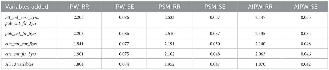
Table 1. Result of DBLP dataset.

If we include more variables, such as the ranking of the authors' respective schools, the average citations of the first author over the past 5 years, the number of citations within 3 years of publication for papers published by the first author in the last 5–10 years, publication date, and so on, using all 13 variables to estimate the propensity score, the results indicate that this ratio is revised to 1.8–1.9.

4 Herring dataset

Every year, the Algemeen Dagblad newspaper organized a competition focusing on the quality of herring. Vollaard and van Ours [2] found that Atlantic-supplied herring received exceptionally high ratings, with an average score of 8.2. In contrast, the herring supplied by other outlets had an average score of 5.5. Furthermore, despite Atlantic's market share being <10%, their herring occupied more than half of the top ten positions in 2016 and 2017. To examine the fairness of these ratings, a regression analysis was conducted, considering factors such as cleanliness, ripeness, freshness, verbal judgment and “Atlantic” (indicating whether herring is supplied by Atlantic). The results revealed that the coefficient for the variable indicating whether the herring was supplied by Atlantic was significant at the 5% level. Considering that one of the critics responsible for the ratings had a vested interest in Atlantic, the authors concluded that the ratings exhibited a bias toward Atlantic, suggesting an unfairness in the evaluation process.

The average score of herring supplied by Atlantic is higher than that of other outlets. There may be two possible reasons for this situation. On one hand, there might be bias in the scoring process favoring Atlantic, which means even if characteristics of the herring are similar, the herring supplied by Atlantic still receives higher score. Therefore whether supplied by Atlantic directly affects the final score. On the other hand, the quality of herring supplied by Atlantic is higher, and this will have an impact on final score and whether they are supplied by Atlantic. The analysis of the characteristics of the two groups of herring is shown in Table 2, indicating a significant difference in the distribution of herring characteristics between Atlantic and other companies. Therefore, the score difference may arise from confounding variables such as maturity, cleanliness, freshness, and linguistic evaluations by critics. Merely relying on the difference in average scores is insufficient to confirm bias toward Atlantic in the scoring process.

Table 2

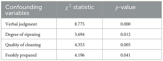
Table 2. Comparison of covariates for herring.

By utilizing linear regression to analyze the relationship between herring scores and the supply from Atlantic, we can partially address the issue of selection bias. However, the model may suffer from endogeneity issues, such as the quality of herring not being fully captured by the features, which is a real concern. The temperature feature of the herring is omitted in the regression analysis, and the verbal comments about temperature are also ignored. Additionally, there could be a non-linear relationship between the herring features and final score and whether the supply from Atlantic is correlated with the residual term in linear regression. All of these could lead to significant coefficient test results.

Indeed, PS methods cannot fully address endogeneity issues. But potential correlations often exist between confounding variables, such as the temperature and freshness of herring, where higher temperatures typically lead to quicker spoilage and reduced freshness. These correlations provide an opportunity to approximate unobserved variables. Linear models are limited to capturing linear relationships. Tree-based models can more accurately calculate proxies for unobserved variables, therefore they can partially mitigating endogeneity issues. Christos Louizos et al. [15] employed variational autoencoders to approximate the joint distribution of observed and unobserved variables and got a more precise estimation.

To test the hypothesis of non-linearity, we attempt to include interaction terms of variables in the linear model. Due to the fact that all variables are categorical factors in linear regression, the number of variables becomes significantly large compared to the limited sample size. In order to reduce the number of variables, we first select splitting points for the variables and then discretize them into factor types. For instance, we choose 1 and 2 as splitting points for the linguistic evaluations of critics, resulting in three variables: (0, 1](1, 2] and (2, 5]. Similarly, we select 1 and 3 as splitting points for cleanliness and maturity variables. After including quadratic and partial cubic interaction terms of these variables in the linear regression, the coefficient for Atlantic is no longer significant. Therefore, we cannot conclude that there is bias in favor of the Atlantic in the scoring solely based on regression analysis.

After adding interaction terms of variables in the linear regression models of Vollard et al., the coefficient test results of Atlantic changed. This may indicates a non-linear relationship between the score of herring and its features. However, continuously adding higher-order interaction terms of variables to approximate the regression function in the linear regression model may lead to overfitting issues. In the subsequent analysis, we attempt to use PS methods to analyze the herring dataset. As shown in Table 3, the p-values of the coefficients of Atlantic are all not significant which indicates that we cannot conclude a significant difference in scores between herring provided by Atlantic and those provided by other companies if their quality is similar.

Table 3

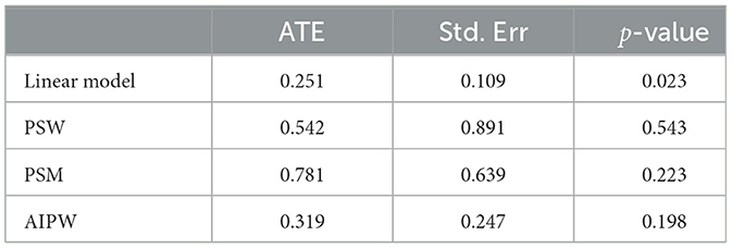
Table 3. Result of herring dataset.

5 CLHLS dataset

Cheng et al. [3] analyzed the Chinese Longitudinal Healthy Longevity Survey (CLHLS) dataset from 2008 to examine how education affects people's health. They used Instrumental Activities of Daily Living (IADL) as a measure of health status among the elderly. They considered baseline characteristics such as education status, gender, age, ethnicity, and parental longevity etc. They progressively introduced health behavior variables and socioeconomic variables into the analysis. The health behavior variables included smoking, alcoholism, diet, exercise, and leisure index. The socioeconomic variables included financial independence, source of livelihood, control over household expenses, health insurance, and medical care. Incorporating these variables led to an increase in the coefficient for the education variable, particularly when including diet, exercise, and leisure index. In all regression analyses, the coefficient for education was found to be statistically significant. This indicated that education could influence physical health by affecting health behaviors and economic capabilities. Among these factors, the effects resulting from influencing diet, exercise, and the leisure index were found to be the most significant. Furthermore, even after controlling for these variables, education continued to have an impact on health.

We recalculate the regression results, as shown in Table 4. The coefficient for education is consistent with the original findings, indicating that our variable selection and handling align closely with the original study. By utilizing the PS methods on this dataset to analyze the impact pathway, we observe that the impact of education on physical health is no longer significant when including the leisure index as a confounding variable while controlling for baseline characteristics. This suggests that educated elderly individuals tend to engage in a more enriching leisure lifestyle, which contributes to better health outcomes. However, when incorporating other health behavior variables, contrary to the linear regression model used in the original study, the coefficient for education decreases. Therefore, we can not conclude that education promotes physical health by influencing other health behavior variables such as balanced diet.

Table 4

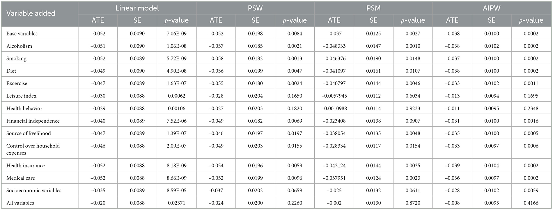
Table 4. Result of CLHLS dataset.

Besides, socioeconomic has a certain influence on health status. After including all socioeconomic variables, the impact of education on health is higher than that of including all health behavior variables. This indicates that healthy lifestyle has a greater impact on physical health than economic capabilities, consistent with the findings of the original study.

After including both health and socioeconomic variables, the impacts of education on health all remain insignificant. It means controlling for these two categories of variables, we can not conclude that education still has an effect on health. In other words, when controlling for baseline characteristics, if an elderly individual does not receive education but possesses a healthy lifestyle and favorable economic conditions, their likelihood of being physically healthy would still be substantial. So we can not establish a relationship between education and health in such cases.

In the original linear regression model, after controlling for socioeconomic and health behavior variables, the impact of education on health remained significant. This could be due to the presence of nonlinear relationships between some variables and health, which can not be captured by linear regression. Additionally, there might be multi-collinearity between education and other variables. To test this hypothesis, we introduce some nonlinear elements into the original regression model (including interaction terms of all variables with education, as well as squared terms for non-binary variables). We find that the coefficient for education was no longer significant. In the new regression model, certain interaction terms between health behavior and socioeconomic variables and baseline characteristics are found to have an impact on health. For example, the p-value for the interaction term between age and alcohol consumption is 0.0035, indicating that older individuals who consume alcohol tend to have poorer health conditions. The p-value for the interaction term between gender and control over household expenses was 0.0051, suggesting that if males have control over household expenses, their health status tends to be worse. However, in the original regression model the coefficient for gender is not significant which indicates that gender does not have a significant impact on health. This may suggests the presence of nonlinear relationships between health and other variables, and using a linear function to approximate is inappropriate. With the inclusion of interaction terms, after controlling for health behavior variables and socioeconomic variables, we can not establish a correlation between education and health. This finding aligns with the results obtained from the PSW method.

6 Simulation

Cepeda et al. [16] pointed out that in situations with a large number of features and a small number of samples, using propensity score method for estimation has advantages over logistic regression in terms of bias, empirical power, and robustness. We analyze three scenarios where the ATE of Z is examined with a true value of 0. We repeated the experiment 100 times and compared the mean, standard error, and p-values of different estimators. The experimental results are shown in Table 5. In most cases, PS methods especially AIPW method, exhibit smaller biases and standard errors compared to linear regression.

Table 5

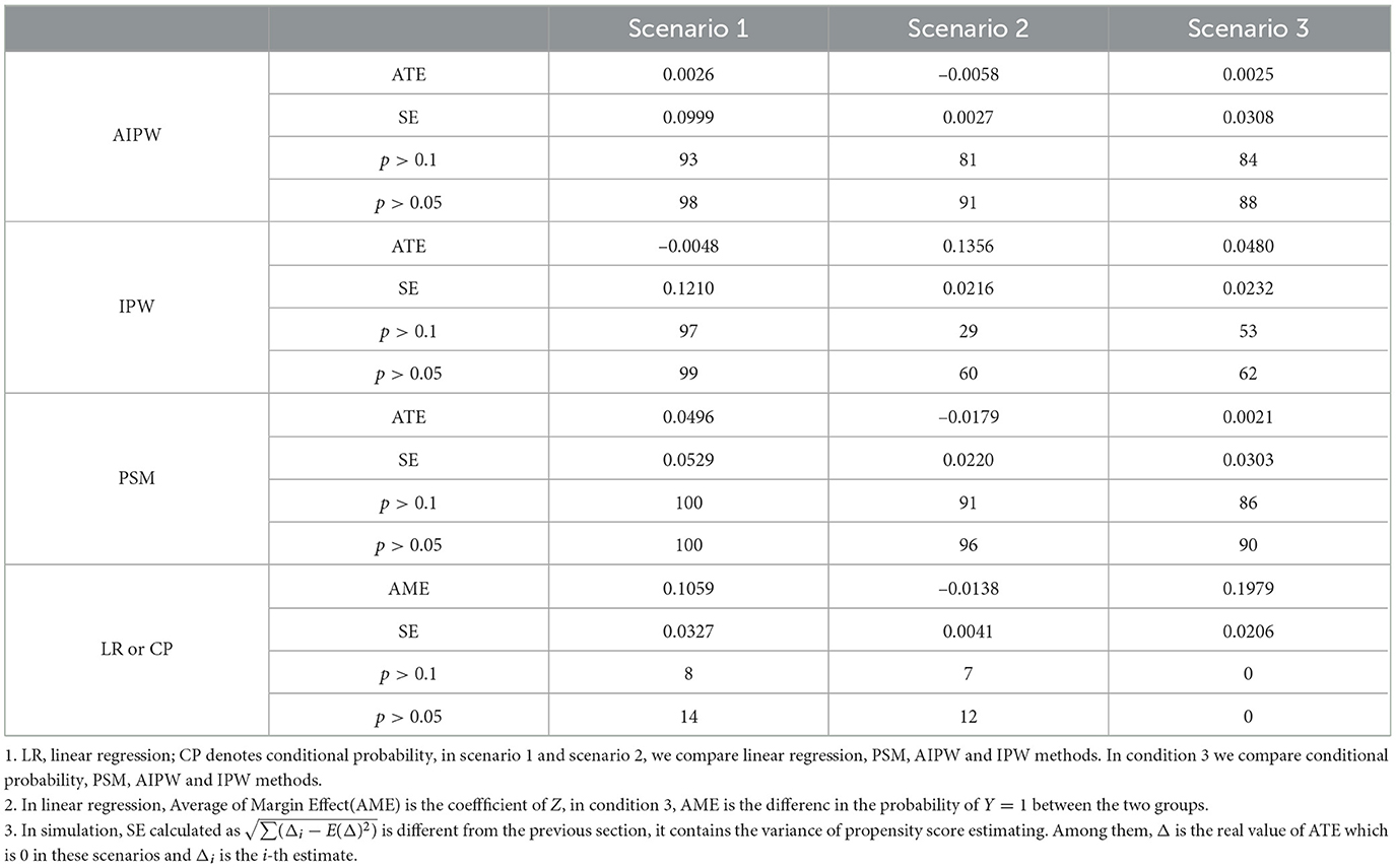
Table 5. Result of simulation.

The first scenario is set as follows,

$\begin{array}{r}Z~B(1,0.3),\\ X_1~N(0.5Z+0.5,0.5),\\ X_2~N(0.2Z+X_1,0.5)),\\ Y=X_1+X_2+0.5\exp (X_2).\end{array}$

where N(μ, σ²) refers to a normal distribution with mean μ and variance σ², B(1, p) refers to the Bernoulli distribution with parameter p. In this scenario, treatment variable Z only affects the observed values through the influence of confounding variables. The analysis results of the PS methods show that after controlling for confounding variables, the coefficients of the experimental treatment variable is no longer significant. This phenomenon is similar to what was observed in the analysis of the CLHLS dataset where linear assumption may not hold. In the results of the linear regression, the education has significant coefficients. However, when analyze using the PS methods and controlling for confounding variables, it appears to be insignificant.

The second scenario is set as follows,

$X_1~N(0,1),$

$X_2~U(0,1),$

$X~B(1,s(0.5X_1+0.6log(X_2))),$

$Y=X_1+X_2+1.5exp(X_2).$

where s(x) = (1+exp(x))⁻¹ is sigmoid function. In this situation, confounding variables can simultaneously affect both the outcomes and the treatment. However, the treatment has no causal effect on the observed values. Additionally, due to the presence of nonlinear terms, the results obtained from linear regression analysis still show that the coefficient of the treatment variable is significant. However, when analyzed using PS methods, this effect is no longer significant. This is similar to what we observed when analyzing the herring dataset.

The third scenario is similar to the second scenario in terms of setup, with the difference being that in the third scenario Y ∈ {0, 1}, and ,

$Z~B(1,s(1.5X_1+0.6log(X_2))),$

$Y~B(1,s(X_1+0.3X_2+0.5\exp (X_2)).$

In this situation, if we directly calculate the probability of y = 1 for the control and treatment group, there is an average difference of 0.20, and all the test results are significant. However, the treatment variable Z has no effect on the observed variable Y. The difference in the probability of Y = 1 between the two groups is entirely due to the influence of confounding variables. Therefore, the effect of the treatment should be close to zero in order to accurately reflect the actual situation. After eliminating the influence of confounding variables using PS methods, the treatment effects are estimated to be nearly zero. This phenomenon is similar to what was observed when analyzing the DBLP dataset, where the novelty and conventionality of a paper, along with confounding variables, can affect the number of citations. After removing the influence of confounding variables, the estimated impact of novelty and conventionality on citation counts decreases.

7 Conclusion

In this paper, we discuss the issue of selection bias in datasets from three different fields: scientific research, natural biology, and demography. Comparing the difference in responses or the conditional probability of Y = 1 between the treatment and control groups directly can lead to estimation bias. To mitigate this problem, some researchers choose to incorporate confounding variables into the analysis framework using linear regression, which can partially alleviate the issue. However, linear regression imposes rather strict assumptions on the model, so relying solely on linear model analysis may lead to erroneous conclusions, as discussed in Section 6 of this paper. In this study, we employ PS methods for analysis. PS methods addresses this problem by weighting or matching the samples to decouple the impact of treatment and confounding variables on the outcomes and estimate treatment effects more accurately. This suggests that it is necessary to compare different methods in decision-making and adjust them based on actual data to avoid making erroneous judgments.

Data availability statement

The raw data supporting the conclusions of this article will be made available by the authors, without undue reservation.

Author contributions

YZ: Formal analysis, Investigation, Methodology, Software, Writing – original draft, Writing – review & editing.

Funding

The author(s) declare that no financial support was received for the research, authorship, and/or publication of this article.

Conflict of interest

The author declares that the research was conducted in the absence of any commercial or financial relationships that could be construed as a potential conflict of interest.

Publisher's note

All claims expressed in this article are solely those of the authors and do not necessarily represent those of their affiliated organizations, or those of the publisher, the editors and the reviewers. Any product that may be evaluated in this article, or claim that may be made by its manufacturer, is not guaranteed or endorsed by the publisher.

References

1. Uzzi B, Mukherjee S, Stringer M, Jones B. Atypical combinations and scientific impact. Science. (2013) 342:468–72. doi: 10.1126/science.1240474

PubMed Abstract | Crossref Full Text | Google Scholar

2. Vollaard B, van Ours JC. Bias in expert product reviews. J Econ Behav Organ. (2022) 202:105–18. doi: 10.1016/j.jebo.2022.08.002

Crossref Full Text | Google Scholar

3. Cheng L, Zhang Y, Shen K. Understanding the pathways of the education-health gradient: evidence from the Chinese elderly. China Econ Q. (2014) 1:305–30. doi: 10.13821/j.cnki.ceq.2015.01.016

Crossref Full Text | Google Scholar

4. VanderWeele TJ. Principles of confounder selection. Eur J Epidemiol. (2019) 34:211–9. doi: 10.1007/s10654-019-00494-6

Crossref Full Text | Google Scholar

5. Rosenbaum PR, Rubin DB. The central role of the propensity score in observational studies for causal effects. Biometrika. (1983) 70:41–55. doi: 10.1093/biomet/70.1.41

Crossref Full Text | Google Scholar

6. Stuart EA. Matching methods for causal inference: a review and a look forward. Stat Sci. (2010) 25:1. doi: 10.1214/09-STS313

PubMed Abstract | Crossref Full Text | Google Scholar

7. Rosenbaum PR, Rubin DB. Reducing bias in observational studies using subclassification on the propensity score. J Am Stat Assoc. (1984) 79:516–24. doi: 10.1080/01621459.1984.10478078

Crossref Full Text | Google Scholar

8. Hirano K, Imbens GW, Ridder G. Efficient estimation of average treatment effects using the estimated propensity score. Econometrica. (2003) 71:1161–89. doi: 10.1111/1468-0262.00442

Crossref Full Text | Google Scholar

9. Robins JM, Rotnitzky A, Zhao LP. Estimation of regression coefficients when some regressors are not always observed. J Am Stat Assoc. (1994) 89:846–66. doi: 10.1080/01621459.1994.10476818

Crossref Full Text | Google Scholar

10. Li Zw, Liu Jm, Ren AG. Introduction to an individual-based standardization method-propensity score weighting. Zhonghua Liu Xing Bing Xue Za Zhi. (2010) 31:223–6. doi: 10.3760/cma.j.issn.0254-6450.2010.02.024

PubMed Abstract | Crossref Full Text | Google Scholar

11. Thomas M, Miller DP, Morrissey TW. Food insecurity and child health. Pediatrics. (2019) 144:e20190397. doi: 10.1542/peds.2019-0397

Crossref Full Text | Google Scholar

12. Yang W, Tang J, YI D, LI X, Wang X, Zhou X. GBM propensity score weighting for causal inference research. World Sci Technol-Modernization Tradit Chin Med. (2017) 1462–72.

Google Scholar

13. McCaffrey DF, Ridgeway G, Morral AR. Propensity score estimation with boosted regression for evaluating causal effects in observational studies. Psychol Methods. (2004) 9:403. doi: 10.1037/1082-989X.9.4.403

PubMed Abstract | Crossref Full Text | Google Scholar

14. Tang J, Zhang J, Yao L, Li J, Zhang L, Su Z. ArnetMiner: extraction and mining of academic social networks. In: KDD'08. San Jose, CA (2008). p. 990–8. doi: 10.1145/1401890.1402008

Crossref Full Text | Google Scholar

15. Louizos C, Shalit U, Mooij JM, Sontag D, Zemel R, Welling M. Causal effect inference with deep latent-variable models. In: Advances in neural Information Processing Systems. Long Beach, CA (2017). p. 30.

Google Scholar

16. Cepeda MS, Boston R, Farrar JT, Strom BL. Comparison of logistic regression versus propensity score when the number of events is low and there are multiple confounders. Am J Epidemiol. (2003) 158:280–7. doi: 10.1093/aje/kwg115

PubMed Abstract | Crossref Full Text | Google Scholar