Removability conditions for anisotropic parabolic equations in a computational validation

1 Introduction

In this article, we investigate singularities of solutions of anisotropic parabolic equations, and in particular the ones of the anisotropic porous medium equation. We focus on conditions for the removability of singularities for such solutions and compare analytically obtained removability results with observed solution behavior in numerical simulations.

For quasilinear elliptic equations, the problem can be formulated as follows. Let Ω be an open subset in ℝⁿ. The function u is defined in Ω\{x₀} and satisfied some quasilinear partial differential equation in Ω\{x₀}, i. e., except in the point x₀ where a singularity might lie. The removability problem consists of extending the function u to the entire domain Ω so that the extended function ũ satisfies the same quasilinear equation in Ω, and in finding conditions that guarantee the existence of the extension. If the extension of u to ũ is possible, we will say that the singularity in x₀ is removable.

Additionally, while dealing with equations of parabolic type like done in this article, singular initial data arise in a natural way. The problem statement remains the same, but it can be formulated in different ways: either as the question of a removable singularity or as the non-existence of a solution with a singularity.

The qualitative behavior of solutions to quasilinear elliptic and parabolic equations near the point singularity was investigated by many authors starting from the seminal paper of Serrin [1]. Further analysis of sufficient conditions for the removability of singularities of solutions has been made by many authors for different classes of nonlinear elliptic and parabolic equations, cf. [2] and the references therein. As for anisotropic elliptic and parabolic equations, their active research began recently. There are many scientists who presented fundamental results in the qualitative theory for such equations. Feo, Vázquez, Volzone, Song, Jian deal with questions about the existence of a fundamental solution [3], self-similar fundamental solutions [4, 5], existence and uniqueness of a bounded and continuous solution for equations with singular advections and absorptions [6, 7]. Skrypnik and his co-authors obtained removability results for the anisotropic versions of the porous medium equation and for the fast diffusion equation [8], the p-Laplacian equation [9] and doubly nonlinear anisotropic parabolic equations [10], including equations with an absorption term [11–16], etc.

The paper is organized as follows. In Section 2, we introduce the statement of the singularity problem for anisotropic parabolic equations. In Section 3, we provide the history of the removability problem for isotropic and anisotropic equations. In Section 4, we present the analytical results on the growth behavior of solutions near the singularities, which are validated and visualized by hands of numerical simulations in Section 5. The paper finishes with a resume and an outlook.

2 Problem statement

We study non-negative solutions to the anisotropic parabolic equation

$\begin{array}{ll}\frac{\partial u}{\partial t}-{\displaystyle \sum _{i=1}^n}\frac{\partial }{\partial x_i}(u^{m_i-1}\frac{\partial u}{\partial x_i})=0\text{ with }(x,t)\in {\Omega }_T,& (1)\end{array}$

where Ω_T = Ω × (0, T), Ω is a bounded open set in ℝⁿ with n≥2, which without loss of generality, contains the origin, i. e., x₀ = 0 ∈ Ω, and where T with 0 < T < +∞ is a finite time. The initial condition is

$\begin{array}{ll}u(x,0)=0\text{ for all }x\in \Omega \backslash \left\{0\right\},& (2)\end{array}$

and allows a concentrated essential weight in the origin.

Eq. (1) can be seen as a diffusion equation for the concentration u = u(t, x), and the diffusion parameters depend on the concentration u as well as on the direction in ℝⁿ via the different exponents m_i−1. The exponents m_i, which are not necessarily integers, have a strong physical background. In fact, they come from fluid dynamics in anisotropic media. If the conductivities of the media are different in different directions, the exponents m_i are different from each others [17].

In the special case m₁ = m₂ =...m_n = 1, Eq. (1) reduces to the isotropic heat equation. But for m_i>1, i = 1, …, n, the diffusion parameters tend to zero with decreasing concentrations. Thus, the diffusion process degenerates near zero concentrations. In this case, Eq. (1) is degenerate parabolic, and it is called an anisotropic porous medium equation [18]. On the other hand, for m_i < 1, i = 1, …, n, the equation is singular parabolic and called anisotropic fast diffusion equation [19].

As we see, the anisotropy of Eq. (1) is realized via the exponents m_i−1 in the concentration-dependent diffusion parameters $u^{m_i-1}$. The case m_i>1 means that the diffusion strength increases with a growing positive concentration u, where m_i < 1 leads to a diffusion strength that increases up to infinity for decreasing u tending to 0. Therefore for small u and m_i < 1, we expect the faster leveling behavior the smaller u is in x_i-direction.

Here, we consider the case when anisotropy exponents are restricted by two conditions, namely first, a lower bound

$\begin{array}{ll}{\displaystyle \underset{1\le i\le n}{min}}{m}_i>1-\frac{2}{n},& (3)\end{array}$

and next, an upper bound depending on the mean of the exponents

$\begin{array}{ll}{\displaystyle \underset{1\le i\le n}{max}}{m}_i<m+\frac{2}{n}\text{where }m=\frac{1}{n}{\displaystyle \sum _{i=1}^n}{m}_i.& (4)\end{array}$

As a first idea, conditions (3) and (4) mean that the exponents m_i might be commonly large but might not differ too much or be too small, comp. Section 4.2, where the admissible anisotropies are investigated in more detail. These conditions cover also the case where one part of the exponents m_i is greater than 1 and the other part m_i is less than 1.

Remark 1. In all known related publications, the cases of degenerate (m_i>1, i = 1, …, n) and singular (m_i < 1, i = 1, …, n) parabolic equations were considered independently from each other even in the isotropic case, i. e. for m₁ = m₂ =... = m_n = m. The used methods for proving the results depend on either the degenerate or singular character of equations.

Remark 2. Without loss of generality, we will assume that the point $x_0=0\in {ℝ}^n$ carries a singularity, otherwise we can make a change of variable by a simple translational shift.

Remark 3. Initial condition (2) can be written in the following way

$\begin{array}{l}u(x,0)=\delta (x),x\in \Omega .\end{array}$

In this case, it will be about the non-existence of solutions to the Cauchy problem with a singular initial condition, and not about the removability conditions.

Here, we are interested in solving the problem (1, 2) numerically and testing the analytical results from [8] which guarantee that the singularity at (0, 0) is removable.

3 History of the problem

The first theorem on removable singularities was obtained by Riemann. In his doctoral dissertation [1851, see Riemann [20]], he established the removability of an isolated singular point for a harmonic function of two real variables. In the general case, the necessary and sufficient condition of the removable singularity at the point x₀ for a harmonic function u in ${ℝ}^n\backslash \left\{x_0\right\}$ has the form

$\begin{array}{ll}u(x)=o(\epsilon (x-x_0))\text{as }x\to x_0.& (5)\end{array}$

Here

$\begin{array}{ll}{\epsilon }_n(x-x_0)=\{\begin{array}{l}\frac{|x-x_0{|}^{2-n}}{(2-n){\sigma }_n},n>2,{\sigma }_n-\text{surface areas of}\\ \text{ the unit sphere in }{R}^n\\ \frac{1}{2\pi }\ln \frac{1}{|x-x_0|},n=2\end{array}& (6)\end{array}$

is the fundamental solution of Laplace's equation that exhibits the solution with the “minimal” singularity at x = x₀. It's easy to see how the condition (Equation 5) works if we expand the harmonic function into a series of spherical harmonics under the following form

$\begin{array}{ll}u(x)=ũ(r,\sigma )={\displaystyle \sum _{i=0}^{\infty }}{\epsilon }^{(i)}(r){\psi }_i(\sigma )+{\displaystyle \sum _{i=0}^{\infty }}{r}^i{\tilde{\psi }}_i(\sigma ),& (7)\end{array}$

where r, σ are the spherical coordinates in ${ℝ}^n\backslash \left\{x_0\right\}$, and ψ_i(σ), ${\tilde{\psi }}_i(\sigma )$ spherical harmonics of degree n. If we assert that the condition (Equation 5) is satisfied, i.e., ũ(r, σ) = o(ε(r)) as r → 0, then the first term on the right side in Equation (7) is missing. It means that u is a harmonic function in the whole ℝⁿ. So this condition shows that there is no solution of Laplace's equation which is singular at the point x₀ and satisfies condition (Equation 5). It is obvious that the question of the removability of the singularity is conditioned by the growth of u near this point. If for example $ũ(r,\sigma )=O({\epsilon }^b(r))$ as r → 0, for some nonnegative integer b, then u admits an asymptotic expansion of the following form

$\begin{array}{l}u(x)=ũ(r,\sigma )={\displaystyle \sum _{i=0}^b}{\epsilon }^{(i)}(r){\psi }_i(\sigma )+{\displaystyle \sum _{i=0}^{\infty }}{r}^i{\tilde{\psi }}_i(\sigma ),\end{array}$

and stays harmonic in ${ℝ}^n\backslash \left\{x_0\right\}$. Therefore, a crucial step in studying the singularity problem is the knowledge of an a priori estimate of u near the singularity.

Then for a long time, the only study of singularity problems dealt with linear equations and with radial solutions of Laplace's equation with nonlinear sources or absorptions. In fact, the first breakthrough is due to Serrin [1] who obtained the first general results on quasilinear equations. His precise condition on removability of singularity for nonnegative solutions of the p-Laplacian equation

$\begin{array}{l}{\displaystyle \sum _{i=1}^n}\frac{\partial }{\partial x_i}(|\nabla u{|}^{p-2}\frac{\partial u}{\partial x_i})=0\text{ for }x\in \Omega \backslash \left\{x_0\right\},\end{array}$

reduces to

$\begin{array}{l}u(x)=o(\epsilon (x-x_0))\text{as}x\to x_0\text{ for }p\le n,\end{array}$

where ε(x−x₀) is the fundamental solution of the p-Laplacian equation and is described by the formula

$\begin{array}{ll}\epsilon (x-x_0)=\{\begin{array}{l}|x-x_0{|}^{-\frac{n-p}{p-1}},\text{ for }p<n,\\ \ln \frac{1}{|x-x_0|},\text{ for }p=n.\end{array}& (8)\end{array}$

Around 1980, the sharp development of the theory of nonlinear partial differential equations allowed another breakthrough in the study of nonradial singular solutions of Laplace's equations with nonlinear sources and absorptions. This was initiated by Gidas and Spruck [21], Lions [22] and Veron [23]. After this first period, many articles have been published taking into account the different aspects of the singularity problem for the above-mentioned equations and also for parabolic equations. We refer to the monograph by Veron [2] for an account of these results.

During the last decade, there have been growing interest and substantial developments in the qualitative theory of second-order anisotropic elliptic and parabolic equations e.g., [5, 24–30], in particular results for anisotropic porous medium equation can be found in Ciani and Henriques [31], Feo et al. [4], Henriques [32], Song and Jian [3], Song [6], and Song [7]. The study of these equations is complicated by the fact that a general qualitative theory for them has not been constructed, in addition, the explicit form of the fundamental solution is unknown in most of the cases. Therefore, the problem arises of obtaining precise conditions for the removability of the singularities for anisotropic elliptic and parabolic equations. Due to the fact that it is not possible to construct the fundamental solution of Equation (1) in an explicit form similar to Equations 6, 8, until recently it was not clear how to formulate the precise or at least sufficient condition for the removability of the singularity for the solution of this equation. This question was successfully solved in Namlyeyeva et al. [10], where is proved that the singularity at the point (x₀, t₀) with x₀ = 0∈ℝ and t₀ = 0 for the solution of the equation

$\begin{array}{l}\frac{\partial u}{\partial t}-{\displaystyle \sum _{i=1}^n}{(u^{(m_i-1)(p_i-1)}|\frac{\partial u}{\partial x_i}{|}^{p_i-2}\frac{\partial u}{\partial x_i})}_{x_i}=0,\\ \text{with}{p}_i\ge 2,m_i\ge 1,\text{and}i=1,\dots ,n,& (9)\end{array}$

is removable if the following condition holds

$\begin{array}{l}u(x,t)=o(z(x,t))\text{ as }(x,t)\to (x_0,0),\end{array}$

where is $z(x,t)={\left({\displaystyle \sum _{i=1}^n|x_i-x_i^0{|}^{{\alpha }_i}+t^{\beta }}\right)}^{-n}$, and the exponents are given by

$\begin{array}{l}{\alpha }_i=\frac{1}{p+n(p(m-d)-m_i(p_i-1))}\\ \text{and }\beta =\frac{1}{n(p(m-d)-1)+p}\end{array}$

with

$\begin{array}{l}m=\frac{1}{n}{\displaystyle \sum _{i=1}^n}{m}_i,p=\frac{1}{n}{\displaystyle \sum _{i=1}^n}\frac{1}{p_i},\text{and }d=\frac{1}{n}{\displaystyle \sum _{i=1}^n}\frac{m_i}{p_i}.\end{array}$

The anisotropic doubly nonlinear parabolic (Equation 9) reduces to the anisotropic p-Laplacian evolution equation if m₁ = m₂ =... = m_n = 1. Further for p₁ = p₂ =... = p_n = 2, we obtain the degenerate case of Eq. (1). Other results on the removability of singularities for anisotropic equations concern special cases of Eq. (9) with absorption [11] and gradient absorption terms [12] and for anisotropic elliptic equations [9, 13–15]. But at this stage of the study, we are not interested in equations with additional terms.

4 Results and visualization

4.1 Removability result for anisotropic parabolic equation

Before presenting sufficient conditions for the removability of singularities, let us formulate the definition of a weak solution of the problem (Equation 1, 2), and let us define removable singularities.

Definition 1. We write V_m(Ω_T) for the class of functions φ∈C(0, T, L²(Ω)) with

${\displaystyle \sum _{i=1}^n}{\displaystyle \underset{{\Omega }_T}{\iint }}\left|\phi {|}^{m_i-1}\right|\frac{\partial \phi }{\partial x_i}{|}^2\text{d}x\text{d}t<\infty .$

Definition 2. A weak solution with a singularity at the point (0, 0) of the problem (Equations 1, 2) is a function u(x, t)≥0 satisfying the inclusion $u\psi \in V_m({\Omega }_T)\cap L^2(0,T,W^{1,2}(\Omega ))$ and the integral identity

$\begin{array}{l}{\displaystyle \underset{\Omega }{\int }}u(x,\tau )\phi \psi \text{d}x-{\displaystyle \underset{0}{\overset{\tau }{\int }}}{\displaystyle \underset{\Omega }{\int }}u\frac{\partial (\phi \psi )}{\partial t}\text{d}x\text{d}t\\ +{\displaystyle \sum _{i=1}^n}{\displaystyle \underset{0}{\overset{\tau }{\int }}}{\displaystyle \underset{\Omega }{\int }}{u}^{m_i-1}{u}_{x_i}\frac{\partial (\phi \psi )}{\partial x_i}\text{d}x\text{d}t=0& (10)\end{array}$

for any 0 < τ < T, any test function $\phi \in V_m({\Omega }_T)\cap L^2(0,T,W_0^{1,2}(\Omega ))$ and any $\psi \in C^1({\overline{\Omega }}_T)$ vanishing in a neighborhood of (0, 0).

Definition 3. We say that the solution of the problem (Equations 1, 2) has a removable singularity at the point (0, 0) if the integral identity (Equation 10) holds for ψ≡1.

According to Def. 3, the u is integrable over the neighborhood of the point (0, 0) supporting the singularity. Hence, the singularity cannot be too strong or not too widely opened, i.e. $u=O(\frac{1}{r^{\alpha }})$ with restricted exponent α. Here u is formally L₁ in the combined space for x and t, and that means that a solution with singular initial values decreases fast enough for growing t.

Theorem 1. Assume that the conditions in Equations (3, 4) are fulfilled. Let u be a weak solution of the problem (1, 2) with a singularity at the point (0, 0). Then the singularity of the solution u is removable if

$\begin{array}{ll}u(x,t)=o(v(x,t))\text{ as }(x,t)\to (0,0),& (11)\end{array}$

where $v(x,t)={\left({\displaystyle \sum _{i=1}^n|x_i{|}^{k_i}+t^k}\right)}^{-n}$ with

$\begin{array}{l}{k}_i=\frac{1}{2+n(m-m_i)}\text{ and }k=\frac{1}{n(m-1)+2}.\end{array}$

The condition (Equation 11) can be rewritten in the following form

$\begin{array}{ll}{\displaystyle \underset{(x,t)\to (0,0)}{lim}}\frac{u(x,t)}{v(x,t)}=0.& (12)\end{array}$

It is natural to expect that v(x, t) determines the asymptotic behavior of the fundamental solution. We know about the existence of the fundamental solutions [3], and for anisotropic fast diffusion equation, the existence and uniqueness of the self-similar fundamental solutions [4]. Since the explicit form of the fundamental solution is unknown, we are dealing with a sufficient condition of the removability for Eq. (1), and not with a precise one.

4.2 Admissible anisotropies

The conditions (Equations 3, 4) restrict the possible exponents m_i, i = 1, …, n from below and from above. Whereas (Equation 3) contains a constant restriction from below (Equation 4) rather restricts the deviation from the mean value m of the exponents.

In the two-dimensional case with n = 2, conditions (Equations 3, 4) read

$m_i>0\text{ and }{m}_i<m+1\text{ for }i=1,2.$

Figure 1 illustrates the set of all admissible exponents in the case n = 2. We start with the inclined line m₁+m₂ = 2m with all pairs (m₁, m₂) with the same mean value m. Due to m_i<m+1, each exponent may not deviate further than 1 from m, and we get a stripe, cf. thick line, and gray stripe in Figure 1.

Figure 1

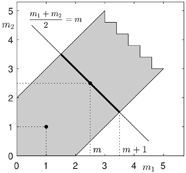
Figure 1. Set of admissible anisotropies in the two-dimensional case n = 2. The gray domains shows all admissible pairs (m₁, m₂) with respect to conditions (3) and (4).

A similar consideration provides the set of admissible exponents in the three-dimensional case with n = 3. Then, inequalities (Equations 3, 4) read

$m_i>\frac{1}{3}\text{ and }{m}_i<m+\frac{2}{3}\text{ for }i=1,2,3.$

The left plot in Figure 2 starts with the plane m₁+m₂+m₃ = 3m containing all triples (m₁, m₂, m₃) with the same mean value. The marked dot gives the isotropic triple (m, m, m). The plane is restricted by the planes $m_i=m+\frac{2}{3}$, which are parallel to the axis-planes of the coordinate system. In the shown situation in Figure 2, left, the lower restriction is not present. If the lower restriction $m_i>\frac{1}{3}$ becomes active, we get a slightly more complicated admissible area, cf. the right plot in Figure 2.

Figure 2

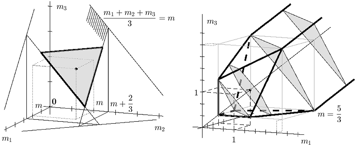
Figure 2. Left: Construction of all admissible triples (m₁, m₂, m₃) with m = 1. The hatched plane gives all triples with m = 1, and the gray triangle is the sub-area restricted by $m_i<m+\frac{2}{3}$, i = 1, 2, 3. Right: Set of admissible anisotropies in the three-dimensional case n = 3. The gray intersections show the admissible areas for $m=\frac{2}{3}$, m = 1, $m=\frac{5}{3}$ and $m=\frac{7}{3}$. Remark the restrictions $m_i>\frac{1}{3}$ for i = 1, 2, 3.

The right plot in Figure 2 presents the three-dimensional set of admissible triples (m₁, m₂, m₃). Additionally, the intersections which were already shown in the left plot, are drawn. These are the rotated triangle for $m=\frac{2}{3}$, a hexagon for m = 1, a two next triangles in gray for $m=\frac{5}{3}$ and $m=\frac{7}{3}$.

Larger $m>\frac{5}{3}$ with inactive condition (Equation 3) lead to triangles and the set of admissible exponent triples is a triangular prism around the diagonal of the positive part of ℝ³. In total, we see a prismatic beam with a triangle cross section and a diagonal in the symmetry axis of the beam. This triangle beam is restricted for small exponents m_i by planes following condition (Equation 3). Analogous beams are found for higher dimensions n>3, too.

Consequently, the analytical and numerical considerations presented in this article, are valid for moderate differences between the exponents m_i in Eq. (1). Otherwise, the mean value m itself, generating the non-linearity in Equation 1 is not limited.

5 Numerical validation

Here, we present the numerical solution of Eq. (1) with the initial condition (Equation 2). It is solved by finite differences, and the singularity in the initial condition was replaced by a particular value conserving the integral. Of course, finite differences are not the ideal method to handle highly oscillating or highly changing values, and rather finite elements with their integrative aspect over each element would be appropriate.

But on the other hand, finite differences are a method which is not related to the removability condition in Eq. (10), which is an integral identity directly connected to the weak formulation of Eq. (1) and thus to finite elements. Therefore, we regard finite differences as a properly unbiased method. By the way, no qualitative difficulties occurred with the numerical solution in Matlab (as used here), Python, or Octave.

Figures 3, 4 show the time evolution of the concentrated initial value in Eq. (2) for n = 2. After a small time, the expected leveling behavior together with an anisotropy close to the origin is observable.

Figure 3

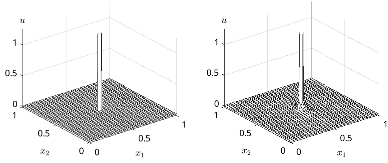
Figure 3. Numerical solution u = u(t, x) of Eq. (1) with m₁ = 1.3 and m₂ = 0.6. Left: Numerical approximation of the initial condition (2). Right: Small t = 0.3·10⁻³ provides a first leveling and a visible anisotropy close to the foot of the former positive values in the origin.

Figure 4

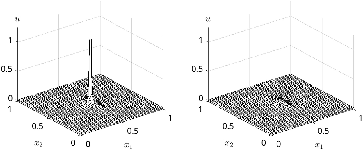
Figure 4. Numerical solution with increasing times, continuation, same m₁ = 1.3 and m₂ = 0.6. Left: Further smoothing for t = 0.6·10⁻³. Right: For t = 0.9·10⁻³, the initial values have been nearly completely leveled out.

Next, we test the limit behavior given in Equation 11 as a removability condition. We compare the numerical solution u = u(t, x) for certain times t>0 with the estimate function v used in Eq. 12 to give an upper bound in the limit x → 0 and t → 0. Figure 5 shows the claimed small-o behavior of u, s. conditions (Equations 11, 12). Please remark that the comparison for t = 0 is not reasonable due to the vanishing initial values outside the origin. Although the small-o behavior of the estimate is numerically reproduced, the computed solution goes a little faster to 0 than the estimate. This coincides with the reformulation of the removability condition (Equation 12).

Figure 5

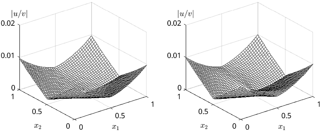
Figure 5. Comparison: Quotient between u(·, x) and the behavior estimate v in condition (Eq. 11). Left: Close to the initial time t = 0.1·10⁻³. Right: Later for t = 0.5·10⁻³, the estimate is less perfect, in particular close to the origin for x → 0 some disturbances are visible.

We observe that the quotient u/v of condition (Eq. 12) is indeed bounded and tends numerically to zero when (x, t) approaches the point (0, 0) carrying the singularity at the initial time. Furthermore, we see that the qualitative tendency observed in the numerical data u is well estimated by the analytical estimate v because the quotient approaches linearly zero in all directions.

Remark that no numerical artifacts are remarkable although the finite differences are a very rough numerical method. Together with the argument that the finite difference method is not biased as e. g. finite elements would be due to the condition in Eq. (10), which would make a non-removable singularity numerically not accessible at the same time, we rate the numerical simulation as a good validation and strong support of the power of the analytical estimate v in condition (Eq. 11).

6 Resume and outlook

We have shown that the removability conditions from [8] for the anisotropic porous medium equation and fast diffusion equation can be numerically reproduced and validated for the admissible anisotropies, whereat the conditions on feasible anisotropies allow not too large differences in the exponents m_i on the one hand but sufficiently multifaceted situation for modeling various physical situations.

Further research will focus on expanding the considerations of removability conditions to more general partial differential equations, e.g. anisotropic version of the evolution p−Laplacian equation. Another interesting question is whether some anisotropies with large differences between the exponents might lead to a comparable behavior of the solutions or whether some extenuated assertations about the growth and decay behavior of the solution can be found.

Data availability statement

The original contributions presented in the study are included in the article/supplementary material, further inquiries can be directed to the corresponding author.

Author contributions

MS: Conceptualization, Formal analysis, Writing – original draft, Writing – review & editing. DL: Conceptualization, Validation, Visualization, Writing – original draft, Writing – review & editing.

Funding

The author(s) declare that financial support was received for the research, authorship, and/or publication of this article. This work was supported by the Volkswagen Foundation project “From Modeling and Analysis to Approximation”, and by the European Union as part of a MSCA4Ukraine Postdoctoral Fellowship.

Acknowledgments

We acknowledge support by the Open Access Publication Funds of Technische Universität Braunschweig.

Conflict of interest

The authors declare that the research was conducted in the absence of any commercial or financial relationships that could be construed as a potential conflict of interest.

Publisher's note

All claims expressed in this article are solely those of the authors and do not necessarily represent those of their affiliated organizations, or those of the publisher, the editors and the reviewers. Any product that may be evaluated in this article, or claim that may be made by its manufacturer, is not guaranteed or endorsed by the publisher.

References

1. Serrin J. Isolated singularities of solutions of quasilinear equations. Acta Math. (1965) 113:219–40. doi: 10.1007/BF02391778

Crossref Full Text | Google Scholar

2. Veron L. Singularities of Solution of Second Order Quasilinear Equations. Longman, Harlow: Pitman Research Notes in Mathematics Series. (1996).

Google Scholar

3. Song BH, Jian H. Fundamental Solution of the Anisotropic Porous Medium Equation. Acta Mathematica Sinica. (2005) 21:1183–90. doi: 10.1007/s10114-005-0573-x

Crossref Full Text | Google Scholar

4. Feo F, Vázquez JL, Volzone B. Anisotropic fast diffusion equations. Nonlinear Analy. (2023) 223:113298. doi: 10.1016/j.na.2023.113298

Crossref Full Text | Google Scholar

5. Feo F, Vázquez JL, Volzone B. Anisotropic p-Laplacian evolution of fast diffusion type. Adv Nonlinear Stud. (2021) 21:523–555. doi: 10.1515/ans-2021-2136

Crossref Full Text | Google Scholar

6. Song BH. Anisotropic diffusions with singular advections and absorptions. I: Existence. Appl Math Lett. (2001) 14:811–16. doi: 10.1016/S0893-9659(01)00049-0

Crossref Full Text | Google Scholar

7. Song BH. Anisotropic diffusions with singular advections and absorptions. II: Uniqueness. Appl Math Lett. (2001) 14:817–23. doi: 10.1016/S0893-9659(01)00050-7

Crossref Full Text | Google Scholar

8. Shan MA. Removable isolated singularities for solutions of anisotropic porous medium equation. Annali di Matematica Pure ed Applicata. (2017) 196:1913–26. doi: 10.1007/s10231-017-0647-2

Crossref Full Text | Google Scholar

9. Namlyeyeva Yu V, Shishkov AE, Skrypnik II. Isolated singularities of solutions of quasilinear anisotropic elliptic equations. Adv Nonlinear Stud. (2006) 6:617–41. doi: 10.1515/ans-2006-0407

Crossref Full Text | Google Scholar

10. Namlyeyeva Yu V, Shishkov AE, Skrypnik II. Removable isolated singularities for solutions of doubly nonlinear anisotropic parabolic equations. Appl Analy. (2010) 89:1559–74. doi: 10.1080/00036811.2010.483426

Crossref Full Text | Google Scholar

11. Sha5n MA. Removability of an isolated singularity for solutions of anisotropic porous medium equation with absorption term. J Mathemat Sci. (2017) 222:741–9. doi: 10.1007/s10958-017-3328-1

Crossref Full Text | Google Scholar

12. Shan MA, Skrypnik II. Keller-Osserman estimates and removability result for the anisotropic porous medium equation with gradient absorption term. Mathematische Nachrichten. (2019) 292:436–453. doi: 10.1002/mana.201700177

Crossref Full Text | Google Scholar

13. Skrypnik II. Removability of isolated singularities for anisotropic elliptic equations with gradient absorption. Isr J Math. (2016) 215:163–179. doi: 10.1007/s11856-016-1377-7

Crossref Full Text | Google Scholar

14. Skrypnik II. Removability of an isolated singularity for anisotropic elliptic equations with absorption. Mat.Sb. (2008) 199:85–102. doi: 10.1070/SM2008v199n07ABEH003952

Crossref Full Text | Google Scholar

15. Skrypnik II. Removability of isolated singularity for anisotropic parabolic equations with absorption. Manuscripta Math. (2013) 140:145–78. doi: 10.1007/s00229-012-0534-5

Crossref Full Text | Google Scholar

16. Skrypnik II. Removability of isolated singularities of solutions of quasilinear parabolic equations with absorption. Mat. Sb. (2005) 196:1693–713. doi: 10.1070/SM2005v196n11ABEH003727

Crossref Full Text | Google Scholar

17. Bear J. Dynamics of Fluids in Porous Media. New York: American Elsevier. (1972) p. 800.

Google Scholar

18. Vázquez JL. The Porous Medium Equation: Mathematical Theory, Oxford Mathematical Monographs. Oxford: The Clarendon Press, Oxford University Press. (2007).

Google Scholar

19. Vázquez JL. Smoothing and Decay Estimates for Nonlinear Diffusion Equations. Equations of Porous Medium Type. Oxford: Oxford Lecture Series in Mathematics and Its Applications 33 Oxford University Press, (2006).

Google Scholar

20. Riemann B. Grundlagen für eine allgemeine Theorie der Functionen einer veränderlichen complexen Grösse (Dissertation thesis). Göttingen: D.R. Wilkins.(1851).

Google Scholar

21. Gidas B, Spruck J. Local and global behaviour of positive solutions of nonlinear elliptic equations. Comm Pure Appl Math. (1980) 34:525–98. doi: 10.4236/apm.2017.711039

Crossref Full Text | Google Scholar

22. Lions PL. Isolated singularities in semilinear problems. J Diff Eq. (1980) 38:441–450. doi: 10.1016/0022-0396(80)90018-2

Crossref Full Text | Google Scholar

23. Veron L. Comportement asymptotique des solutions d'equations elliptiques semilineairesdans R^N. Ann Mat Pura Appl. (1981) 127:25–50. doi: 10.1007/BF01811717

Crossref Full Text | Google Scholar

24. Boccardo L, Gallouët T, Marcellini P. Anisotropic equations in L₁. Diff Integral Equat. (1996) 9:209–12. doi: 10.57262/die/1367969997

Crossref Full Text | Google Scholar

25. Buryachenko K, Skrypnik I. Riesz potentials and pointwise estimates of solutions to anisotropic porous medium equation. Nonlinear Analy. (2019) 178:56–85. doi: 10.1016/j.na.2018.07.006

Crossref Full Text | Google Scholar

26. Ciani S, Mosconi S, Vespri V. Parabolic Harnack Estimates for anisotropic slow diffusion. J d'Analyse Mathemat. (2023) 149:611–642. doi: 10.1007/s11854-022-0261-0

Crossref Full Text | Google Scholar

27. Ciani S, Vespri V. An introduction to barenblatt solutions for anisotropic p-laplace equations. Springer INdAM Series (2021) 43:99–125. doi: 10.1007/978-3-030-61346-4_5

Crossref Full Text | Google Scholar

28. Ciani S, Skrypnik II, Vespri V. On the local behavior of local weak solutions to some singularanisotropic elliptic equations. Adv Nonlinear Anal. (2023) 12:237–265. doi: 10.1515/anona-2022-0275

Crossref Full Text | Google Scholar

29. Lieberman G. Gradient estimates for anisotropic elliptic equations. Adv Diff Equat. (2005) 10:767–812. doi: 10.57262/ade/1355867831

Crossref Full Text | Google Scholar

30. Liskevich V, Skrypnik II. Hölder continuity of solutions to an anisotropic elliptic equation. Nonlinear Anal. (2009) 71:1699–708. doi: 10.1016/j.na.2009.01.007

Crossref Full Text | Google Scholar

31. Ciani S, Henriques E. A brief note on Harnack-type estimates for singular parabolic nonlinear operators. Bruno Pini Mathem Analy Seminar. (2023) 14:56–76. doi: 10.6092/issn.2240-2829/18849

Crossref Full Text | Google Scholar

32. Henriques E. Concerning the regularity of the anisotropic porous medium equation J Math Anal Appl. (2011) 377:710–31. doi: 10.1016/j.jmaa.2010.10.077

Crossref Full Text | Google Scholar