Estimating Tsunami-Induced Building Damage through Fragility Functions: Critical Review and Research Needs

Introduction

Tsunami are long propagating waves generated by large scale underwater displacements (eg. earthquake, underwater explosions), or aerial impacts (eg. landslides), which travel at high speeds across large bodies of water. When they reach coastal areas, large tsunami can inundate up to several kilometers inland causing many deaths and costly damage or destruction to buildings and infrastructure in the coastal region.

Figure 1 shows a widely accepted definition of risk to natural hazards in the built environment (Crichton, 1999) applied to tsunami. Following recent large tsunamis (e.g., Indian Ocean, 2004; Chile, 2010 and Japan, 2011) significant resources have been dedicated worldwide to improve tsunami hazard models (Suppasri et al., 2016). This has resulted in significant advances being made in the identification of tsunamigenic earthquake sources and their activity (Yamazaki and Cheung, 2011; Satake et al., 2013), and in the modeling of tsunami propagation and inundation both numerically (Synolakis et al., 2008) and experimentally (Rossetto et al., 2011; Goseberg et al., 2013; Foster et al., 2017). Less effort has been dedicated to the prediction of damage to the built environment from tsunami inundation and the accurate evaluation of tsunami risk.

FIGURE 1

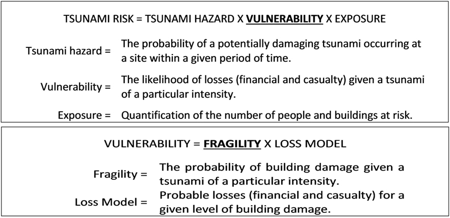
Figure 1. The components of tsunami risk. Fragility is highlighted as it is the focus of this paper.

While some vulnerability assessment methods may directly relate probable losses to tsunami intensity (direct vulnerability), more detailed assessments (indirect vulnerability) separate the assessment of likely building damage (fragility assessment) from the estimation of losses due to that damage (the loss model), as shown in Figure 2. Fragility (sometimes referred to as “physical vulnerability”) relates an indicator of building damage to a measure of the tsunami intensity at the location of each considered building.

FIGURE 2

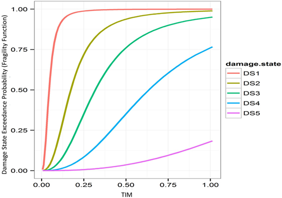
Figure 2. Example fragility functions. IM, intensity measure; DS, damage state. The y-axis represents the probability of damage exceedance for each damage state (P{ds < DS} versus IM).

Fragility functions are a family of cumulative distribution functions that provide the probability of a given type of building exceeding specified damage states (where each individual curve represents a specific damage state, such as “collapse” or “heavy damage”) over a range of values of a tsunami intensity measure (TIM, e.g., inundation depth). In order to derive fragility functions, three components are required: damage data, tsunami inundation data, and the statistical model linking them (i.e., a representation of the mean damage exceedance probabilities and the associated uncertainty). There are in the literature a small number of tsunami damage functions, which relate a TIM directly to mean damage (Ruangrassamee et al., 2006; Valencia et al., 2011); however, these do not consider aleatoric uncertainty at a given TIM value so can be considered superseded by fragility functions, and so they will not be considered further. Vulnerability functions relate a TIM directly to financial loss or casualties (Berryman, 2005; Reese et al., 2007; Masuda et al., 2012) though very few exist in the literature (due partly to challenges in obtaining financial data), and so the remainder of this paper will focus only on fragility functions.

Functions can be classified according to how the damage data are gathered (regardless of how the inundation data are gathered) (D’Ayala et al., 2013; Rossetto et al., 2014). Empirical fragility functions derive damage data from post-tsunami assessments (or physical experiments); judgment-based functions derive damage estimates from expert elicitation; analytical functions use numerical simulations of structural damage (Dias et al., 2009; Park et al., 2013; Kircher and Bouabid, 2014; Macabuag and Rossetto, 2014); and hybrid functions use a combination of these techniques. Empirical fragility functions make up the overwhelming majority of the available functions, and so will be the focus of this paper.

The field of tsunami fragility assessment is relatively new when compared to seismic fragility, and there are, therefore, many lessons that can be learned from the seismic field. However, tsunami fragility assessment has access to damage data of better quality (primarily from the 2011 Great East Japan Earthquake and Tsunami) and so new statistical approaches have been developed that would not have been feasible using currently available earthquake damage datasets.

Tarbotton et al. (2015) give a review of existing literature on tsunami fragility curves, noting trends and comparing existing fragility curves in order to highlight variability in the mean function across a range of studies. However, they do not provide guidance on how to interpret and tackle such variability, nor draw on literature from other fields (such as earthquake engineering), nor include the most recent research that has made significant leaps forward in areas such as critical assessment of the statistical models, multivariate methods, treatment of missing data, and quantification of uncertainty in both the explanatory and response variables of the fragility functions. Note that the terminology used by Tarbotton et al. (2015) to classify fragility functions is different to that of the Global Earthquake Model (GEM), though to be consistent with best practice functions will be classified as empirical or analytical as per the GEM guidance throughout this paper.

The present review provides the most comprehensive review of existing studies to-date and provides a deeper understanding of what drives the epistemic (systematic) uncertainty in existing models, and how to practically reduce it, focusing on sources of uncertainty which can be addressed. Key empirical fragility models from existing literature have been chosen for this purpose, representing a variety of locations, events, statistical approaches, intensity measures, and building stocks most commonly investigated. Drawing upon experience of a similar exercise for the development of the GEM compendium, this paper formulates recommendations consistent with the established best-practice in the seismic field (PAGER, GEM).

The aim of this paper is to collate and summarize existing empirical tsunami fragility functions for buildings, to outline limitations and significant advances in the field, and to propose key areas for further development. The information presented in this paper will allow the reader to assess the quality of current estimations (both based on the quality of the data, and the quality of the models and theories adopted), and to adopt best practice when developing new fragility functions and, therefore has significant implications for those using, assessing, or developing empirical tsunami fragility functions.

Existing Empirical Tsunami Fragility Functions

Empirical fragility functions are based on observed damage data from tsunami events. Table 1 shows existing empirical tsunami fragility functions for the 1993 Japan tsunami, 2004 Indian Ocean tsunami, 2009 Samoa Tsunami, and 2010 Chilean Tsunami. Table 2 shows existing empirical tsunami fragility functions for the 2011 Japan tsunami.

TABLE 1

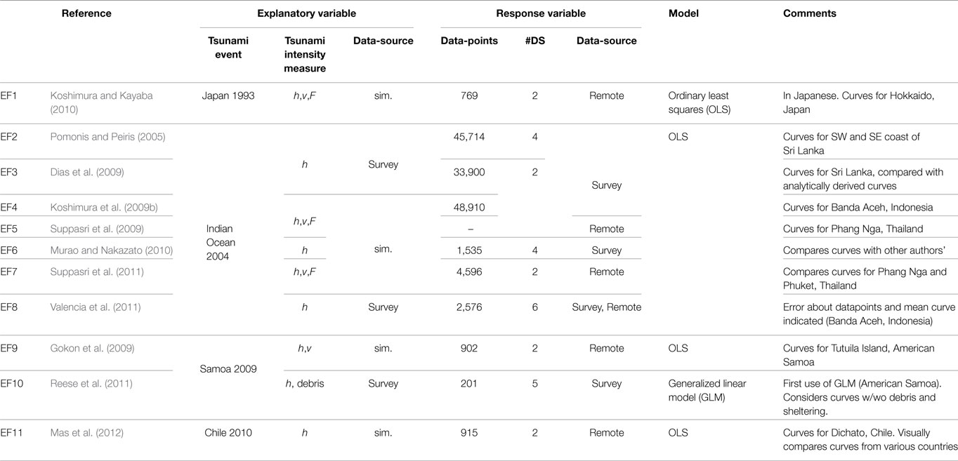
Table 1. Published empirical fragility functions for the 1993 Japan tsunami, 2004 Indian Ocean tsunami, 2009 Samoa Tsunami, and 2010 Chilean Tsunami.

TABLE 2

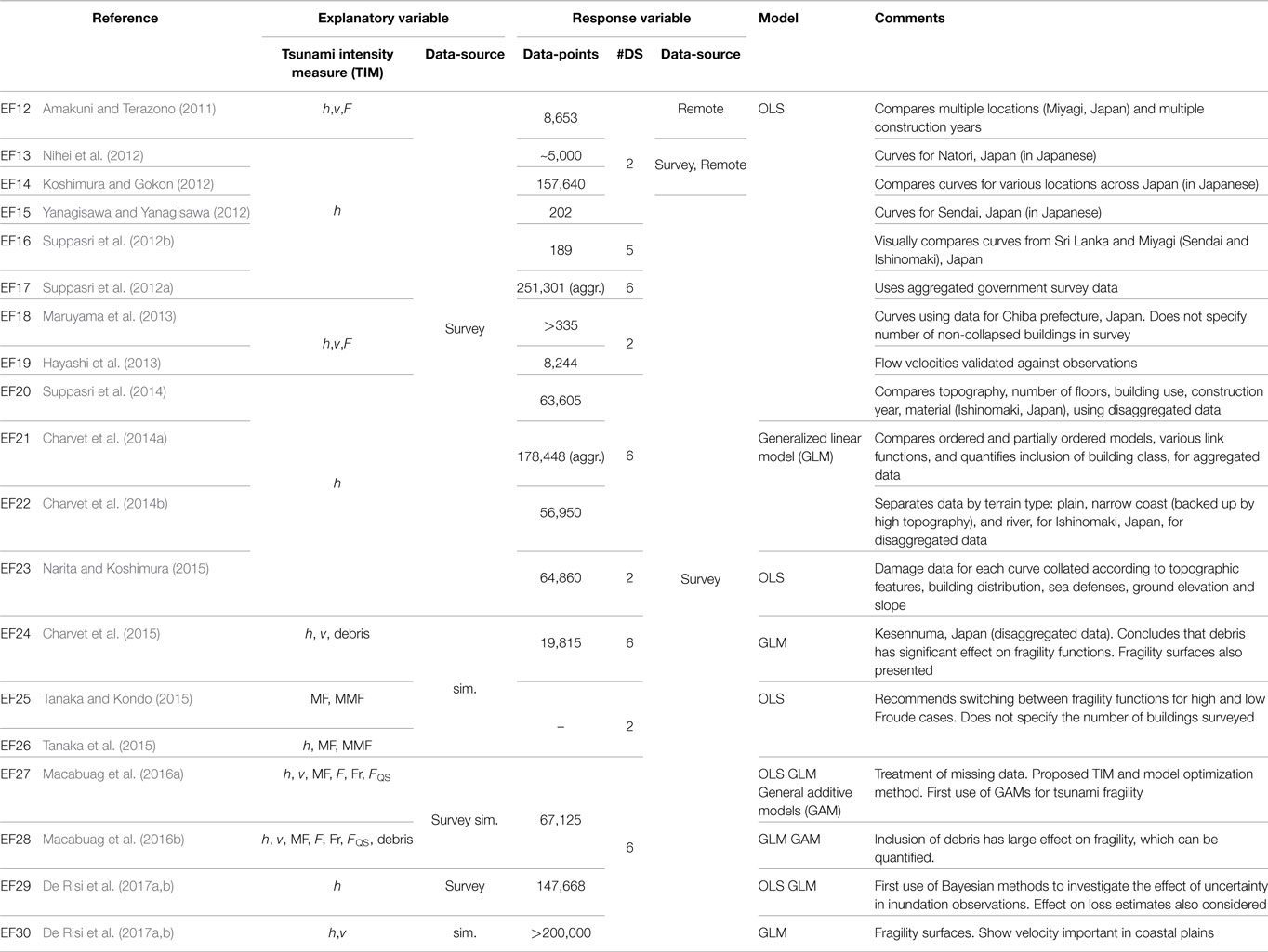
Table 2. Published empirical fragility functions derived from data for the 2011 Great East Japan Earthquake and Tsunami.

In Tables 1 and 2, TIM indicates the TIM assigned to each building, discussed in detail in Section “The Explanatory Variables: Tsunami Intensity Measures” (h, inundation depth; v, velocity; F, drag force; MF, momentum flux; MMF, moment of momentum flux, F_QS, a new proposed quasi-steady force estimate). The explanatory variable data-source describes how the TIM was determined for each building (sim., numerical inundation simulation). The response-variable data-points indicate the number of buildings in the study (− = data not given in the reference, Aggr. = aggregated, note that all data are aggregated when used in OLS models, see Model Quality). Response variable data-source indicates how damage data were collected (remote = satellite or aerial imagery, survey = visual inspection in the field). #DS indicates number of damage states (including DS0, so that #DS = 2 indicates 1 fragility curve, generally collapse). The model column indicates the statistical model describing the fragility function (OLS = standard linear model with parameters estimated via ordinary least squares (OLS), generalized linear model (GLM) using maximum likelihood parameter estimation with various link functions, see Section “Model Quality”).

It can be seen that there are many more fragility functions derived from data for the 2011 Japan tsunami (19 fragility functions) than for all previous tsunamis combined (11 fragility functions), which is indicative of the unprecedented quantity and quality of data that have become available following the 2011 Japan tsunami. Furthermore, it can also be seen that the majority of damage data from the 2011 Japan tsunami which has been used in fragility functions is from field surveys, again due to the unprecedented scale of the surveys conducted, such as that conducted by Japan’s Ministry of Land Infrastructure Tourism and Transport (MLIT) which provided a database of all of the houses (over 200,00) within the tsunami inundation zone.

Existing fragility functions cover several construction types, including engineered structures in Japan (RC, steel, masonry, and timber), and primarily non-engineered structures of Thailand, Indonesia, and Samoa. Some studies consider construction year (Amakuni and Terazono, 2011; Suppasri et al., 2014) and number of stories (Suppasri et al., 2013, 2014), though most do not make this distinction. The majority of studies use normal or lognormal models with OLS parameter estimation, with improved models (e.g., GLM) becoming more widely used in more recent studies.

Alongside the published studies presented in Tables 1 and 2, there are also substantial proprietary investigations carried out by commercial catastrophe risk modeling companies using confidential insurance loss information. While these cannot be included in this paper, the comprehensive review and recommendations presented here are of significance to modelers and model developers interrogating or developing these proprietary functions.

A critical review of this literature is now presented according to the three fundamental components of tsunami fragility functions. Building damage data are discussed in Section “The Response Variable: Building Damage Data,” tsunami intensity data in Section “The Explanatory Variables: Tsunami Intensity Measures,” and the statistical model that links the two in Section “Model Quality.” Finally, recommendations are made regarding areas for future research and current best practices in deriving tsunami fragility functions.

The Response Variable: Building Damage Data

Fragility functions express the probability that a building may reach or exceed a set of damage states, for a given value of a TIM (e.g., inundation depth). Damage states represent the response variable in regression analysis, and each curve of a family of fragility functions represents a different damage state. This section sets out the criteria that an optimal damage scale should meet for fragility function derivation and discusses the current literature in relation to these criteria, highlights shortcomings in damage data collection, and highlights that currently used building classifications miss features of the building that make it vulnerable to tsunami.

Damage Scale

Damage scales define the set of damage states into which tsunami-affected buildings are classified. McCullagh and Nelder (1983) states fundamental rules that damage scales must follow, and Hill and Rossetto (2008) proposed a ranking system for “scoring” existing seismic damage scales based on the key characteristics required for use in loss modeling. The rules and characteristics relevant for tsunami fragility function derivation are shown in Table 3 and the damage mechanisms to be captured by fragility functions are defined and characterized in Table 4. All of the fragility functions derived from data for the Great East Japan Earthquake and Tsunami (Table 2) use the damage scale proposed by the Japan Cabinet Office (2013) shown in Table 5.

TABLE 3

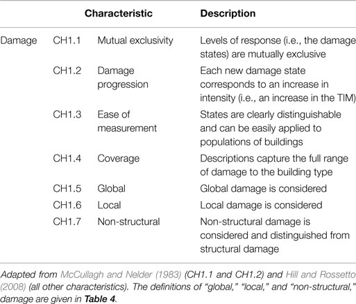
Table 3. Important characteristics of a damage scale for tsunami fragility function derivation.

TABLE 4

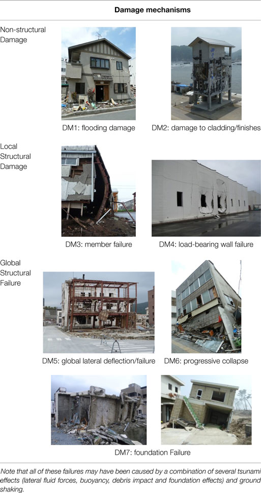
Table 4. Tsunami-induced damage and failure mechanisms (photos: EEFIT).

TABLE 5

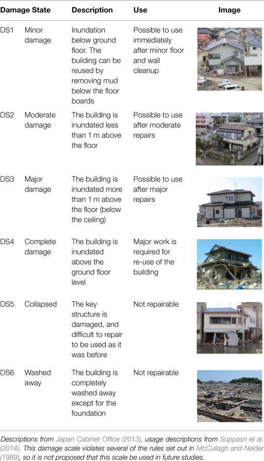
Table 5. Damage state definitions used by the Japanese Ministry of Land Infrastructure Tourism and Transport following the 2011 Great East Japan Earthquake and Tsunami.

The damage scale in Table 5 (and many of the scales presented in Table 1) violates the first rule set out by McCullagh and Nelder (1983) (CH1.1, Table 3). For example, buildings with inundation below the ground floor ceiling (DS3) could also experience collapse (DS5). Therefore, surveyors inspecting a building that falls into multiple damage state categories is presented with a subjective choice as to which damage state to assign. Charvet et al. (2014a,b) highlight that the descriptions of DS5 and DS6 also violate the second rule (CH1.2, Table 3). The damage scale in Table 5 also does not directly address global and local damage nor distinguish between structural and non-structural damage but instead shows an assumed direct correlation between the hazard intensity (inundation depth in this case) and damage in that depth is specified directly in the damage state descriptions for DS1-DS4, and so structural response is not actually considered by these definitions.

The shortcomings of the damage scale in Table 5 have implications for the uncertainty in the observations for empirical studies and, therefore, raises questions about the reliability of existing functions derived from data for the Great East Japan Earthquake and Tsunami (Table 2). Furthermore, the remaining building damage scales that can be found in the literature for tsunami (Table 1) are often not consistent, having different damage state definitions and a varying number of damage states, or otherwise fail to meet the criteria set out above. An improved and unified damage scale is, therefore, required for future studies.

Damage Data: Quality and Collection Method

Empirical building damage data post-tsunami is collected either via ground survey (visual inspection), or remotely (aerial or satellite photography). Remote sensing allows for the rapid collection of large amounts of data. However, the limitation on satellite remote sensing damage surveys is that the only detectable damage state is often “total collapse” (and where intermediate damage states are included, their accuracy is low), meaning that accurate fragility functions cannot be formed for partial collapse states (e.g., all studies in Table 1 utilizing remote sensing consider only two damage states). Construction material can often not be determined remotely. Ground surveys can determine material and intermediate damage states, though they take more time than remote sensing. Ground surveys can be conducted by surveyors with different levels of training and expertise. They are commonly carried out for purposes other than the construction of fragility functions (e.g., for safety evaluations) hence they may not record appropriate damage. Further sources of uncertainty are introduced due to the typical issues highlighted in Table 6.

TABLE 6

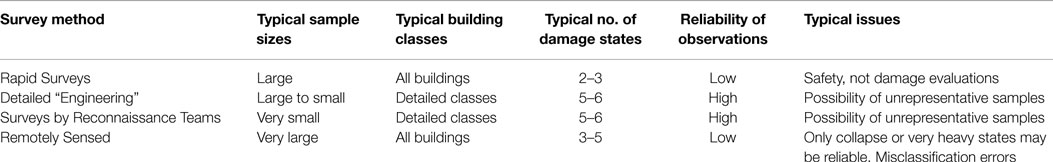
Table 6. Database typologies and their main characteristics [adapted from Rossetto et al. (2014)].

In the case of an earthquake-generated tsunami where damage is surveyed in the near-field regions, it is likely that the earthquake has damaged buildings before the tsunami’s arrival. Park et al. (2013) considered previous seismic damage in an analytical study of tsunami fragility. However, for empirical studies, it is difficult to separate tsunami-induced damage from earthquake-induced damage, which creates bias in the data (Rossetto et al., 2012) and so likely affects the applicability to estimating tsunami-only risk (e.g., for far-field tsunamis) for all of the fragility functions derived from the 2011 Japan tsunami to some degree.

Empirical fragility functions can be very specific to the location from where the damage data were gathered. Suppasri et al. (2014) and Charvet et al. (2014b) compare fragility functions formed using data from areas within the same city (Ishinomaki, Japan) but with different topographies. Narita and Koshimura (2015) separate building damage data by location according to four broad factors: bathymetric features, distribution of buildings, coastal protection facilities, topographic features. Such studies show that fragility functions cannot typically be generalized or applied to similar structures in a different geographical location.

Empirical fragility studies based on field measurements all face the issue of data analysis with missing attributes, and existing studies [e.g., Suppasri et al. (2013)] generally conduct complete-case analysis, i.e., they remove any partial data, such as buildings of unknown material, from their fragility analysis. However, this may lead to a loss of statistical power, loss of precision, and introduction of bias if the missing data are informative. Missing data can be assigned to one of three categories [Ware et al. (2012)]: Missing Completely At Random (MCAR), Missing At Random (MAR), or Missing Not At Random (MNAR). MCAR refers to the case where the data are missing purely by chance. MNAR refers to the case where the missing information is related to the reason that the information is missing (e.g., if wooden buildings had been removed from the dataset because they were wooden). MAR refers to the case where the information is not MCAR but can be accounted for by using other attributes. The only study to analyze and treat missing data before conducting fragility function derivation is Macabuag et al. (2016a). All other studies that produce fragility functions for various building classifications based on data from existing fragility functions may be susceptible to bias introduced by the removal of incomplete data-entries.

Building Classification

In order for the fragility results to be representative of the different structural responses to tsunami loading, typically buildings are classified according to structural properties and analysis is carried out on each class separately. Suppasri et al. (2014) considers structural material, height, occupancy, and date of construction (concluding that date of construction did not greatly affect tsunami performance). All other existing studies consider structural material only. However, the building classifications are not consistent between studies. For example, Tinti et al. (2011) divides masonry buildings into five sub-classes of structures with varying construction materials and numbers of stories, and Valencia et al. (2011) consider two types of masonry-structures (class B and C). Fragility functions from different studies can often not be compared for this reason.

The purpose of a building classification system is to allow buildings to be grouped according to their likely performance in the case of tsunami, i.e., so that they can be represented by a single set of fragility curves. Current building classes that have been used in tsunami fragility studies are based on classification systems for earthquakes and do not take into account the building characteristics that make buildings susceptible to damage from tsunami (e.g., openings, soil type, foundation type, cladding system). This means that they may cluster together buildings that will perform differently in tsunami, into the same building class. For example, an RC structure with and without large openings will behave very differently in tsunami, or a structure founded on piles verses one on raft foundations may behave very differently even if it has the same superstructure. Therefore, a building classification system that accounts for the features of the building that make it vulnerable to tsunami (so grouping buildings of similar performance together) is presented in Section “Assessment/Improvement of the Quality of Building Damage Data.”

The Explanatory Variables: TIMs

Tsunami intensity measures (represented as the x-axis of fragility curves) should provide the best possible representation of the damage potential of the tsunami. In this respect, they can be considered as trying to represent the structural demand that a given tsunami places on the building being investigated. However, existing studies vary in their selection of TIMs and derivation of intensity data. This section, therefore, compares the various TIMs used in the literature, highlights challenges in their methods of derivation, and highlights that the optimal TIM depends on the particular dataset being used.

Summary of Intensity Parameters

Tsunami-induced building damage can arise due to hydrostatic forces (including buoyancy), hydrodynamic effects (drag and bore impact), and debris (impact and damming), and the severity of these effects are determined by a number of flow parameters.

The majority of existing tsunami fragility curves adopt only the local maximum inundation depth as the TIM (Tables 1 and 2), often because it is the most readily definable parameter from post-tsunami surveys [e.g., residue lines in houses, Suppasri et al. (2012a,b)] and can be calculated from numerical inundation simulations more accurately than other flow parameters (discussed below, Section “Determination of Inundation Parameters”). Flow depth is indeed the main parameter driving lateral hydrostatic forces, buoyancy forces, and it also determines the size of debris that can be carried by the flow. However, a wide range of velocities (and so hydrodynamic forces) can exist for a given inundation depth, and indeed various studies have indicated that the sole use of inundation depth does not adequately describe observed damage at higher damage states (Charvet et al., 2014a; Macabuag et al., 2016a,b). Note also that various definitions and names for inundation depth can be found in the literature [water level (Reese et al., 2007), inundation depth (Inoue et al., 2007), tsunami depth, or water depth (Tanaka et al., 2007)], and so caution should be exercised when referring to these studies.

Flow velocity influences the hydrodynamic force, the surge force, the debris impact, and damming forces. Studies that have compared TIMs have generally concluded that velocity alone is less effective than depth as an indicator of damage for buildings for the datasets investigated (Koshimura et al., 2009a,b; Macabuag et al., 2016a). However, velocity is often used to calculate the fluid force TIMs shown in Table 7.

TABLE 7

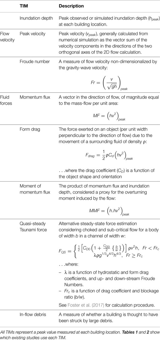
Table 7. Tsunami Intensity Measures (TIMs) used in the current literature.

Froude number indicates the flow regime such that Fr < 1 indicates sub-critical flow (where the flow velocity is less than the wave velocity and so behaves in a slow or stable way) and Fr > 1 indicates choked or supercritical flow (where flow is dominated by inertia forces, so behaving as a rapid or unstable flow). Macabuag et al. (2016a) is the only study to consider Froude Number as a TIM and found it to be a poor indicator of building damage when used alone, for the dataset considered. However, Froude Number is used to calculate the quasi-steady force discussed below (Qi et al., 2014; Foster et al., 2017), and Tanaka and Kondo (2015) recommend using different fragility curves for flow conditions characterized by high and low Froude numbers.

Momentum flux is proportional to hydrodynamic form-drag (Table 7) and so they can be considered equivalent TIMs [i.e., fragility functions derived from momentum flux and drag force will give identical goodness-of-fit results, Macabuag et al. (2016a)]. Park et al. (2014) compares damage estimates for a case-study town in the USA using fragility functions for depth, velocity, and momentum flux, concluding that velocity and momentum flux provide the most realistic damage estimates, though this is only based on a qualitative visual assessment of damage locations and the authors acknowledge that this conclusion must be verified with field data. Tanaka and Kondo (2015) are the only empirical study to consider moment of momentum flux in their fragility curves. Note that nearly all current studies that consider force are using the standard drag equation (all except Macabuag et al. (2016a), below, and Tanaka and Kondo (2015) who additionally consider moment of momentum flux), however, this does not account for alternative estimations, such as equivalent hydrostatic methods (MLIT, 2011), bore impact (Robertson and Riggs, 2011), or changes in flow regime (Qi et al., 2014; Foster et al., 2017).

Macabuag et al. (2016a) derived fragility functions using an equivalent quasi-steady force proposed by Qi et al. (2014) and shown by Foster et al. (2017) to represent the force of a tsunami inundation on buildings. It is evaluated via two different flow regimes determined by Froude number. The equations relate depth, velocity, and blockage ratio (building width/channel width) to the force. Increasing the blockage ratio generally has the effect of increasing the force on the structure, and readers are referred to Qi et al. (2014) for the calculation procedure. Macabuag et al. (2016a) found that measures of force appear to provide the most efficient TIMs, if the inundation simulation from which they are derived is sufficiently accurate, or simulated velocity can be validated, and, furthermore, that flow regime (indicated by Froude number) appears to be a significant consideration when conducting fragility assessments, or quantifying tsunami-induced forces on structures.

Debris impact has been shown to have a significant influence on tsunami-induced damage and has been considered in fragility function derivation by Charvet et al. (2015), Macabuag et al. (2016b), Reese et al. (2011). However, all current studies simply use a binary indicator defining whether a building is thought to have been impacted or not, and further work is needed in order to more fully capture the characteristics of the likely forces imposed by debris on the structure.

Overall, the literature does not show a consensus as to which flow parameter is the most appropriate TIM to estimate fragility, though Macabuag et al. (2016a) proposed a rigorous methodology for determining the optimum TIM for any given dataset.

Tsunami magnitude is not considered a TIM as it is a function of offshore wave characteristics only and is not building specific. Run-up is also not considered a TIM as it is not building-specific, though it can be used to estimate building-specific inundation depths.

Not all tsunami loads and effects are necessarily captured by any single TIM used in the current literature (Table 7). For example, duration of immersion (and number of waves) is not captured in existing TIMs. This is significant as additional waves provide multiple impulsive impacts on the structure, the structure experiences load-reversal due to both the inflow and draw-down, and increases degradation of non-engineered structural materials (e.g., wood). Scott and Mason (2017) propose multi-hazard intensity measures considering both seismic and tsunami demand in a single parameter, though this concept has not been explored for fragility analysis. In fluvial flood modeling, Kreibich et al. (2009) compare Flood Intensity Measures of depth, velocity, momentum flux, and energy head according to the Bernoulli Equation, concluding that for fluvial flooding depth and energy head have the strongest correlation with observed damage, although it is acknowledged that a much larger sample size is required in order to draw conclusive results.

Froude Number and all of the force TIMs presented in Table 7 are all complex TIMs that represent information of both depth and velocity. However, even a complex TIM may not capture all the relevant tsunami information necessary to predict structural damage, and so it would be beneficial to consider additional intensity measures simultaneously. Multiple regression techniques allow for several intensity measures to be included in the model simultaneously. Charvet et al. (2015) and De Risi et al. (2017a,b) generate fragility surfaces considering depth and velocity simultaneously (Figure 3), both concluding that such multiple regression models are more accurate than considering either TIM in isolation. However, surfaces are currently seldom used in practice for quantitative loss estimation and it is always the aim to develop a “parsimonious model” (the best model for the fewest predictors) as using additional intensity measures requires more data points and difficulties of obtaining these additional tsunami parameters must be overcome.

FIGURE 3

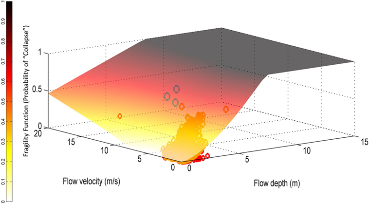
Figure 3. Example tsunami fragility surface showing building collapse probability conditional on two key intensity measures, flow depth and velocity. Adapted from Charvet et al. (2015).

Determination of Inundation Parameters

For the derivation of fragility functions, the flow conditions at each building location (i.e., the TIM values) must be measured or estimated. These flow conditions may be obtained from post-tsunami field surveys, or they can be calculated using empirical flow estimation methods or numerical inundation modeling techniques. Calculation of onshore flow, by either empirical or numerical methods, requires information of offshore conditions obtained by modeling propagation from source to the coastline. Source and deep-sea propagation modeling is beyond the scope of this study, but methods of inundation estimation based on offshore conditions will be briefly discussed here, as the accuracy of the resulting TIM values directly impacts the reliability of the final fragility functions.

Field Surveys

In post-tsunami field surveys, flow depth can be measured using for example local water marks, or debris hanging on trees. If flow depth cannot be measured directly from an affected building (for example, the building has been washed away) various interpolation methods can be employed to estimate parameters between observation location (Mas et al., 2012; De Risi et al., 2017a,b), though there will be error introduced by the interpolation. Note that run-up may also be obtained from field surveys in order to validate numerical inundation results, either by direct observation immediately post-tsunami or by examining tsunami deposits, particularly for historic tsunamis.

Flow velocity is difficult to determine from observations in sufficient accuracy and resolution (EEFIT, 2006; Reese et al., 2007), and so is always calculated numerically for fragility function derivation. However, observation methods are often used to validate numerical results (Adriano et al., 2016).

Tsunami-induced forces on buildings have never been directly measured, and although some studies have attempted to estimate tsunami forces from observed damage to onshore structures (Tokyo University and BRI, 2011; Chock et al., 2013), force-related TIMs for fragility analysis have always been based on numerical inundation modeling.

Empirical Flow Estimation

Several studies and guidelines provide empirically based approaches for the estimation of onshore depth, velocity, and force.

Inundation depth values used in existing empirical fragility studies have all been derived using either field surveys or numerical modeling, and all velocity values obtained from numerical modeling. However, empirical methods may be used to verify numerical results in specific locations. These empirical methods include, for example, empirical formulae to estimate run-up from off-shore flow parameters [Charvet et al. (2013)], formulae provided by FEMA (2012) for determining the peak depth and velocity field from the run-up, or the energy grade-line method proposed by ASCE 7-16 (Kriebel et al., 2017) using offshore tsunami amplitude and run-up maps to define peak onshore depth and velocity fields.

However, depths and velocities are obtained, all of the fragility studies using any measure of force as a TIM generally use empirical formulations to estimate forces (Table 7) based on the peak depth and velocity flow-fields.

Numerical Inundation Modeling

Numerical modeling of tsunami inundation can provide estimates of onshore flow conditions across large areas as well as at single sites but poses a complex problem in computational fluid dynamics. Inundation models can vary in complexity from detailed 3D models considering flow around individual buildings to simplified 2D models modeling built-up areas using a roughness factor and making assumptions regarding the depth distribution of velocities and pressures (Table 8).

TABLE 8

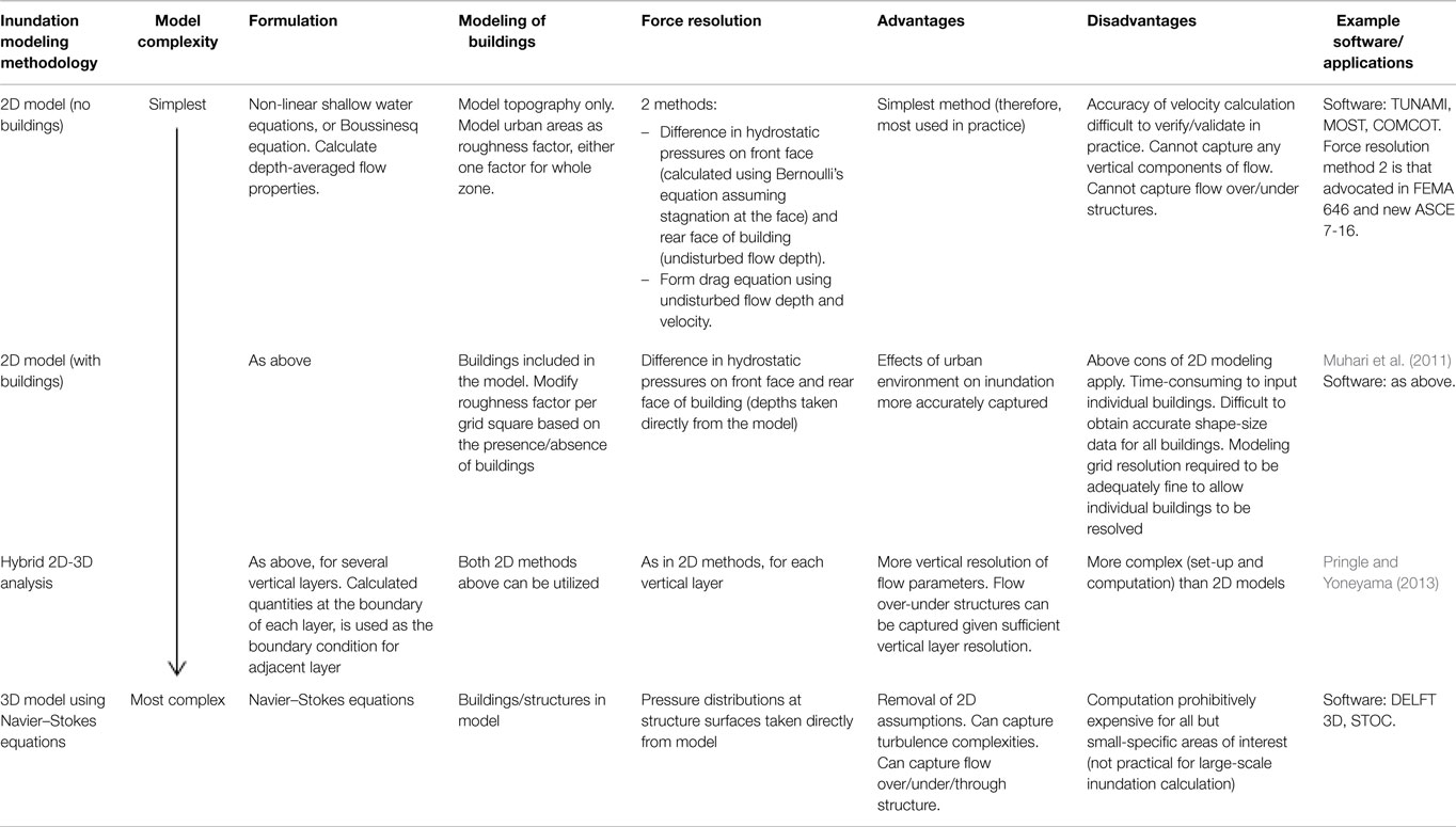
Table 8. A summary of numerical methods that have been used to define tsunami-induced forces on structures.

Tables 1 and 2 show which existing fragility studies obtain TIMs from numerical inundation. Where simulation has been used, simplified 2D models have been utilized as detailed topographical data are often lacking, and more complex models are still prohibitively costly in computation time and the required resources in accurately modeling a location with all buildings and obstacles to the required resolution. The required TIMs are calculated for each grid, and for each timestep, though over a large inundation area this would represent a prohibitively large dataset, and so only peak TIM values are retained.

Existing studies using a force-related TIM (and Froude Number) all rely on empirical formulae to calculate force from depth and velocity. Peak depth and peak velocity generally do not occur at the same time (Chock, 2016), so peak force should not be calculated from the peak values of depth and velocity, but instead force should be calculated at each timestep with the peak force value over the inundation duration being retained for each calculation grid.

Numerical inundation estimates are seen to be highly sensitive to the uncertainties/inaccuracies in the initial properties of the tsunami (shape and total energy), the near-shore bathymetry, the effect of wave breaking, the on-shore topography, the effect of buildings and other obstacles, which may move or alter throughout the inundation period. Furthermore, while it is possible to validate simulated inundation depth results, there is generally insufficient velocity observation data to conduct a meaningful validation (Macabuag et al., 2016a,b). Park et al. (2013) compare simulated depth, velocity, and momentum flux values to experimental results, and Park et al. (2014) conduct a sensitivity analysis of the same TIMs to friction coefficient and modeling software. Both studies find that a change in simulation parameters can lead to small changes in depth, but result in much greater changes in velocity and momentum flux (e.g., they report a 15% change in depth corresponded to a change in velocity and momentum flux of 95% and 208%, respectively).

Therefore, the reliability of the existing fragility functions based on velocity or force is very dependent on the accuracy of those inundation models, which is determined by a number of factors. such as quality/reliability/resolution of the topography/bathymetry data, quality/reliability of the source and propagation models, the software used, the resolution of the calculation grid, and so on.

Model Quality

Fragility functions are derived by applying statistical model fitting techniques on building damage data. They are expressed as a function of the chosen TIMs for the purpose of making damage predictions under future tsunamis. In this context, statistical model fitting assumes that the probability of damage exceedance P_DS is a function of the TIM:

$P_{\mathit{DS}}=P\left(\mathit{ds}\ge \mathit{DS}|\mathit{TIM}\right)=f\left(\mathit{TIM}\right)$ (1)

In Eq. 1, ds is the observed damage state and DS the classification label given by the damage scale.

Three types of statistical models have been used in the literature:

• Linear models that utilize linear least squares regression—most commonly applied in fragility studies (Tables 1 and 2),

• GLM (e.g., Reese et al., 2011; Charvet et al., 2014a; Muhari et al., 2015; Macabuag et al., 2016a,b; De Risi et al., 2017a,b),

• Generalized Additive Models (Macabuag et al., 2016a,b).

This section describes methods of statistical model fitting and model diagnostics used in tsunami fragility studies to date, highlighting potential shortcomings of each method as well as potential solutions and proposed best-practice.

Traditional Fragility Estimation: Simple Linear Regression

Lognormal cumulative distribution functions have been the most popular form of tsunami fragility functions in the literature. This approach is typically attractive given the following three properties of this distribution (Ioannou et al., 2012):

• The lognormal distribution is constrained in the y-axis between [0, 1] which is suitable for fitting data points expressing aggregated probabilities,

• Values of the dependent variable are constrained in [0, +∞], which is sensible when considering parameters such as flow depths,

• This distribution appears to be skewed to the left, thus, it can provide a better estimate for the smaller intensities, where typically the majority of the data lie.

This has become a standard assumption, however, not well justified in the literature [e.g., “The capacity of the structure is generally assumed to be lognormally distributed” (Valencia et al., 2011); “(…) we develop the fragility functions for structural damage and casualties throughout the statistical analysis under the assumption that they can be represented by normal or lognormal distribution functions (…)” (Koshimura et al., 2009a,b)].

However, this distribution applies to a continuous response and, therefore, is not a suitable representation of discrete, classified outcomes such as a damage scale.

Simple linear regression applies when only one explanatory variable at a time can be considered as the TIM (i.e., for defining curves rather than functions of multiple TIMs, such as fragility surfaces). When a lognormal distribution is assumed, the fragility function or expected probability of damage exceedance ${\widehat{P}}_{\mathit{DS}}$ is expressed as follows:

${\widehat{P}}_{\mathit{DS}}\left(\mathit{IM}\right)=\mathrm{\Phi }\left[\frac{\text{log}\left(\mathit{IM}\right)-\mathrm{\mu }}{\mathrm{\sigma }}\right]$ (2)

The parameters μ and σ of the distribution can be estimated using least squares regression by linearizing equation (2), where Φ is the normal distribution function:

$\text{log}\left(\mathit{IM}\right)=\mathrm{\sigma }{\mathrm{\Phi }}^{-1}+\mathrm{\mu }$ (1)

Unfortunately, this model is unable to deal with probabilities of 0 and 1 (the inverse normal distribution function does not converge for those values), thus disaggregated data cannot be analyzed directly. The data need to be aggregated into bins across the TIM to define a total number of buildings (across all damage states), and the number of buildings corresponding to each damage state DS. The observed probability of damage is then calculated as follows:

$P_{\mathit{DS}}\left(\mathit{IM}\right)=\frac{n_{\mathit{DS}}}{n_{\mathit{Total}}}$ (4)

However, aggregation introduces uncertainty: for example, the distribution of the TIM within each bin is unknown, which may affect the shape of the curve, or the number of points in all bins may not be equal. In addition, data aggregation does not prevent some bins from having either a very low or a very high number of damaged buildings, which means that probabilities of 0 and 1 may still exist in the dataset. This issue is usually overcome by dismissing the corresponding data points and has consequences on model performance (Charvet et al., 2014a; Macabuag et al., 2016a).

New Fragility Estimation: GLM

Overview

The aforementioned issues associated with linear models have been addressed in recent research, by using a different class of models, namely GLM. GLMs relax many of the assumptions associated with linear regression and allow the response variable to follow various distributions (McCullagh and Nelder, 1989). Contrary to linear models, GLMs provide a better representation of the post-tsunami data because:

1. Discrete probability distributions (binomial or multinomial) can be used directly to model discrete outcomes, such as a damage level.

2. The linearity assumption (which may not hold) between the response and the explanatory variable (TIM) is relaxed through the use of a linear predictor.

3. More than one TIM can be included in the linear predictor, thus the model is not limited to one explanatory variable.

4. Model fitting does not require aggregation of the observations.

5. If only aggregated data are available, the binomial distribution can be used directly, without the need of a weighting system.

Parameter Estimation

In GLM regression, the assumption that the explanatory variable x is linearly related to the probability of damage ${\widehat{P}}_{\mathit{DS}}$ is relaxed by using a linear predictor η, which relates the probability of damage to all J available explanatory variables x_j through a link function g:

$g\left({\widehat{P}}_{D{S}_k}={\mathrm{\mu }}_k\right)={\mathrm{\eta }}_k={\mathrm{\theta }}_{0,k}+{\displaystyle \underset{j=1}{\sum ^J}}{\mathrm{\theta }}_{j,k}{x}_j$ (5)

Equation 5 is the systematic component of the model, where μ_k represents the expected damage probability function (i.e., fragility function) for each k non-zero damage level. θ_0,k and θ_j,k are the parameters of the model to be estimated through maximum likelihood estimation (McCullagh and Nelder, 1989; Myung, 2003), commonly abbreviated as MLE.

In Eq. 5, g is the link function relating the linear predictor to the mean of the chosen distribution and can take one of the following forms for discrete outcomes:

$\text{Probit}g\left({\mathrm{\mu }}_k\right)={\mathrm{\Phi }}^{-1}\left({\mathrm{\mu }}_k\right)$ (1)

$\text{Logit}g\left({\mathrm{\mu }}_k\right)=\text{log}\left(\frac{{\mathrm{\mu }}_k}{1-{\mathrm{\mu }}_k}\right)$ (7)

$\text{Cloglog}g\left({\mathrm{\mu }}_k\right)=\text{log}\left(-\text{log}\left(1-{\mathrm{\mu }}_k\right)\right)$ (8)

This model requires the response to be expressed in terms of the counts of buildings that have been damaged to a level equal or exceeding a predetermined damage state. The response can be considered to follow either a binomial or multinomial distribution for every level of intensity, and the random component of the model is the chosen distribution.

Logistic regression is the name given to GLM regression when the distribution is assumed binomial and the link function is the logit. It is appropriate when we assume the response variable is binary. However, the ordered nature of damage states is not represented. This may lead to inconsistent results, such as fragility functions that cross (Figure 4, left panel), implying DS_k+1 is reached before DS_k as the intensity measure increases. Multinomial or Ordinal regression are both used when the response variable is defined as a categorical outcome, or classification; however, ordinal regression is a method specific to cases where such outcome is ordered (1, 2, 3…etc.), resulting in the so-called cumulative link model. In ordinal regression, θ_j,k (the rate of change of response probability for a unit increase in x_j) is fixed across damage levels (θ_1,k = θ₁), which preserves response ordering. Figure 4, right panel shows the fragility curves obtained using an ordinal model on the same sample data as in Figure 4, right panel. Table 9 summarizes the components and concepts behind GLM regression.

FIGURE 4

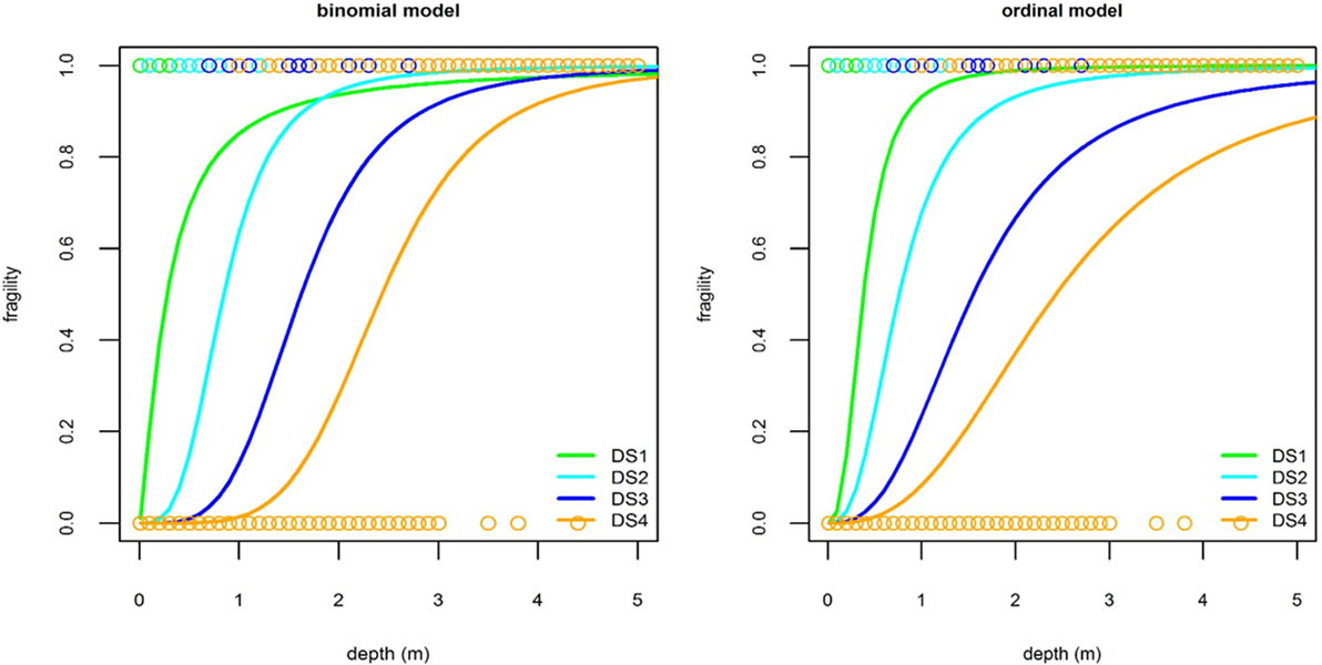
Figure 4. Left—Crossing Fragility Functions—An unrealistic result which can be rectified by using ordinal regression. Here, the binomial logistic model has been fitted to a representative sub-sample of the data used in Charvet et al. (2014b) for illustrative purposes. Right—The same data analyzed using ordinal regression. The cross-over cannot take place.

TABLE 9

Table 9. GLMs used for fragility function derivation.

Generalized Additive Models and Non-Parametric Models

One key assumption made in GLMs is that all explanatory variables are linearly related through the predictor (Eq. 5), which may not be the case. If rigorous diagnostics reveal that the chosen GLM do not provide a satisfactory fit to the data, alternative methods such as general additive models (GAM) or non-parametric regression can be used (Macabuag et al., 2016a).

Generalized additive models [developed by Hastie and Tibshirani (1990)] are semi-parametric models that fit GLMs in a piecewise regression system with a number of separation points (or knots). While there are dangers in using non-parametric and semiparametric methods for prediction purposes due to overfitting (Chandler, 2014), methods for overcoming this issue are demonstrated in Macabuag et al. (2016a). Rossetto et al. (2014) recommend that GAMs can be used if the data do not have a strictly monotonic trend which can be captured by GLMs, and when the data are densely distributed in the available TIM range (>100 data points). The reader is referred to Wood (2006) for detailed instruction on the fitting of GAMs.

When all assumptions cannot be met, an alternative approach is to use non-parametric regression, as non-parametric regression does not require a set of assumptions to be met for the results to be accurate and meaningful. The local polynomial kernel method is presented in Rossetto et al. (2012), this approach consists in using a well-known function (kernel) which is successively centered on each data point and uses a number of surrounding data points (bandwidth) to estimate the resulting function. Kernels are typically used as smoothers in signal processing (Schuenemeyer and Drew, 2011). The issue with this approach is the final, curve is very sensitive to the choice of bandwidth if the latter is too small, the resulting function will pick up unnecessary local variations in the data, if it is too large, the trend might be too general. Therefore, if all parametric alternatives fail to provide a satisfactory fit to the data non-parametric regression can be a useful alternative.

Model Diagnostics

Unfortunately, the evolution of fragility studies applied to tsunami induced damage is still at an early stage and adequate model assessment is seldom carried out. This leads to the impossibility of identifying sources of uncertainty in the probability estimations, thus preventing model improvement. In order for fragility results to be exploited further, it is necessary to perform model diagnostics to reveal if the model used gives a satisfactory representation of the data, identify sources of uncertainty, and assess the adequacy of the systematic and random components.

Diagnostics of Linear Models

For such models, the goodness-of-fit is typically assessed by reporting the value of the coefficient of determination, or R² [e.g., Gokon et al. (2010) and Suppasri et al. (2011)]. However, this assessment of model performance is insufficient in the light of the shortcomings previously outlined in this section.

In addition, when using any form of parametric regression, assumptions should be systematically validated as part of the analysis, as they can be easily violated (Charvet et al., 2013). Linear regression requires several assumptions to be met (Chatterjee and Hadi, 2006), which are typically not checked in practice.

Diagnostics of GLM

For binomial models, it is necessary to graphically examine the model errors (or Pearson residuals, McCullagh and Nelder, 1989) for each curve, which may reveal:

• The non-linear contribution of an additional variable/effect on the model (identification of a trend in the errors),

• Potential inadequacy of the link function,

• Influential points or outliers,

• Over-dispersion (the values of the residuals or errors are more than two standard deviations away from the mean, thus indicating a potential issue in the choice of distribution),

For ordinal and multinomial models, expected versus observed probabilities or counts graphs can be used [Figure 5: Expected versus observed probabilities after fitting an ordinal model to the building damage data, as per Charvet et al. (2014b)—Figure].

FIGURE 5

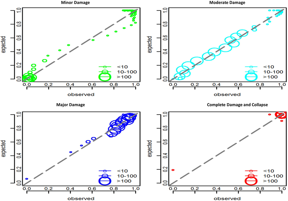
Figure 5. Expected versus observed probabilities after fitting a multinomial model to the building damage data used in Charvet et al. (2014b), for 1 storey timber buildings. The green, light blue, dark blue, and red color codes correspond respectively to DS1, DS2, DS3, DS4 and over, as per damage descriptions in Table 6. A good fit is indicated by counts following closely the 45 line.

Model accuracy (the proportion of correctly classified outcomes) can be used as a quantitative indicator of the performance of the model. It is directly related to the prediction error rate (the proportion of incorrectly classified outcomes). Charvet et al. (2015) propose a penalized accuracy measure (accounting for the distance between observed and expected outcomes) estimated through 10-fold cross-validation, which provides a quantitative assessment of goodness-of-fit of the model and an indication of predictive power. This methodology was applied by Macabuag et al. (2016a) to assess model performance, as well as prevent overfitting with the use of GAMs.

Measures such as the AIC (Akaike Information Criterion) or likelihood ratio tests based on deviance for nested models are useful measures for model comparison. These can only be used to compare two models that have been fitted on the same data and with the same choice of statistical distribution:

• The likelihood ratio test (Rossetto et al., 2014) can be used to assess whether a model with more parameters provides a significantly better fit in comparison to a simpler model with less parameters (i.e., nested models). For example, it can be used to assess whether a model with an additional explanatory variable fits the data significantly better. It can also be used to test the relative goodness-of-fit of the multinomial model compared to the ordinal model, its simpler alternative. Indeed, in an ordinal model, the free parameters for each class are fixed, which leads to a smaller number of parameters in comparison with the multinomial alternative (see Table 9).

• The AIC (Akaike, 1974) can be used, for example, to compare two identical models but differing only by their link function. It can also be used for nested models. The AIC can be calculated as follows:

$\mathit{AIC}=2p-2\text{\hspace{0.17em}log}\left(L\right)$ (9)

$L\left(\mathrm{\theta },\mathrm{\varphi }|\mathit{DS}\right)=P\left(\mathit{ds}=\mathit{DS}|\mathrm{\theta },\mathrm{\varphi }\right)$ (10)

In Eq. (9), −2ln(L) is the model’s deviance (a measure of the model error), p is the number of parameters in the model, ϕ is the dispersion parameter (a function of the model’s variance), and L is the likelihood function (McCullagh and Nelder, 1983). The model that provides the best fit to the data is the model with the smallest AIC.

Various options for model configuration and selection method are presented in Table 10.

TABLE 10

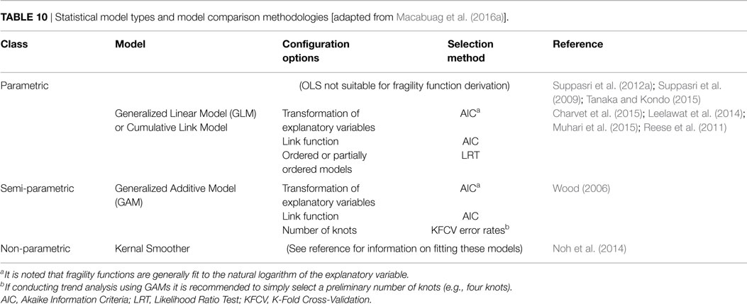
Table 10. Statistical model types and model comparison methodologies [adapted from Macabuag et al. (2016a)].

Further Considerations for Statistical Modeling

Sample Size

A low number of data points may lead to a spuriously well-fitted model (over-prediction). While a minimum sample size must be used to yield reliable results, little guidance is available on its determination (Rossetto et al., 2012).

Comprehensive studies on the topic of sample size have been carried in the context of linear regression, although these considerations also apply to the context of generalized linear modeling. In the context of simple or multiple regression such as linear regression, a rule of thumb states there should be no less than 50 data points for a regression, with the number increasing with larger numbers of independent variables. VanVoorhis and Morgan (2007) and Green (1991) provide a more detailed guidance in the context of regression analysis, based on power considerations.

Leveraging on the results from Cohen (1988), Green (1991) provides power tables that give the required sample size according to the number of predictors and expected effect size, i.e., the strength of the relationship between the predictor(s) and the response. If we assume that, for example, the damage state of a building is strongly related to the tsunami flow depth (i.e., the effect size is large), and flow depth is the only available predictor variable, the aforementioned power table recommends a minimum of 24 points. It should be noted that this study focused on the analysis of data for behavioral sciences, such thresholds should be investigated in the context of the typical relationships expected in physical sciences. Other studies have recommended to use anything from a minimum of 10 (Miller and Kunce, 1973; Harrell et al., 1985; Bartlett et al., 2001; Babyak, 2004) to a minimum of 100 (the case of small effect size or large number of predictors in Green, 1991) or even 200 data points (Guadagnoli and Velicer, 1988; Nunnally and Bernstein, 1994). Ideally, the analyst should carry out their own sensitivity study prior to fitting a statistical model, the minimum number of data points required to construct a vulnerability or fragility function depending on the level of uncertainty the analyst is willing to accept.

However, the scarcity of data is often a limitation and current rules-of-thumb have to be used.

In the case of fragility curves for earthquakes, a minimum of 100 observations is recommended (Rossetto et al., 2014) and at least 30 of them should have reached or exceeded a given damage state (Noh et al., 2014), with the data points spanning a wide range of TIM values. Although there is a reasonable starting point to guide tsunami fragility function derivation, research is needed to assess the minimum sample size for tsunami fragility.

Aggregation of Data

When data are aggregated over bins of the TIM (such as flow depth), it is assumed that the distribution in each bin is normal or uniform (as the value of TIM for each bin is taken as its median). This definition affects both the shape of the function and the confidence intervals. For instance, Valencia et al. (2011) generated 0.1 m wide bins from minimum to maximum flow depth recorded. Similarly Koshimura et al. (2009b) generated 0.2 m bins in order to separate the building damage data into groups of roughly equal size. The definition of bins of arbitrary sizes (x-axis) typically leads to an inconsistent number of buildings in each sample, without the model accounting for points of different weights. This issue may be addressed by weighting the N_i data points in each sample. However, if both a large and small number of data points are used, i.e., 10 < N_i < 100; the smaller samples will not have any influence on the curve and may have to be removed (Ioannou et al., 2012).

Data are also aggregated, at the collection stage, by location, by damage level, or by building class. Aggregation of data over real areas, including variable inundation depths introduces significant uncertainty in the TIM (x-value) at any specific location (Koshimura et al., 2009a). Charvet et al. (2014a,b) found the analysis of the 2011 Japan tsunami damage data aggregated over Japan led to a significant amount of uncertainty in the results, and Macabuag et al. (2016a) quantified the uncertainty related to data aggregation by showing a clear reduction in predictive accuracy of the model.

Finally, data from different sources (for example, different events or survey teams) are often grouped and analyzed as a single entity. This practice does not account properly for all sources of uncertainty. In such cases, it is appropriate to use generalized linear mixed models. These models introduce a random intercept for each group in Eq. (5) to explicitly account for the group (event or survey) as an explanatory variable (Rossetto et al., 2014).

Missing Data

Macabuag et al. (2016a) demonstrate techniques to classify missing data and complete the database accordingly (Table 11). Where data are identified as MCAR complete-case analysis may be conducted without introducing bias in the results. For data that are MNAR, complete-case analysis would introduce bias and missing data cannot be estimated, and so the dataset must be supplemented with additional information to address this issue before fragility analysis can be conducted. For data that are MAR, the missing data may be estimated by Multiple Imputation (MI) techniques. MI involves replacing missing observed data with substituted values estimated multiple times via stochastic regression models built on the other attributes (used as explanatory variables), with all of the imputations being combined in order to derive the final estimate (Rubin, 1987).

TABLE 11

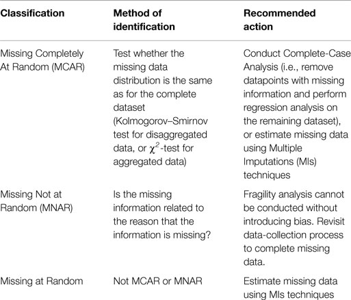
Table 11. Classification and treatment of missing data (adapted from Macabuag et al., 2016a).

Figure 6 demonstrates the effect of bias due to complete-case analysis on fragility function derivation. Macabuag et al. (2016a), therefore, recommends that existing fragility assessments should be re-examined for potential bias if they have been based on complete-case analysis of data subsets (e.g., construction material).

FIGURE 6

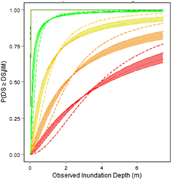
Figure 6. The effect of ignoring incomplete datasets. Dashed-lines show curves formed using complete-case analysis for steel and RC buildings from the 2011 Japan Tsunami (i.e., ignoring all buildings for which the construction material was unknown). Solid lines show a range of mean curves for the imputed dataset (i.e., with building material for “unknown” buildings estimated using MI). Colours indicate the individual damage states, from light damage (dark green) to collapse (red). (Adapted from Macabuag et al., 2016a).

Discussion, Recommendations, and Future Research

Existing tsunami fragility functions are concisely presented in Tables 1 and 2, which summarize the key features of the damage datasets, inundation datasets, and statistical models used by each function. Generally, there is considerable variability in terminology within the studies presented in Table 1. In order to compare and combine fragility functions it is important that consistent terminology is used, and so recommended terminology has been presented for tsunami risk and vulnerability (Figure 1), and the various methods for presenting damage and loss estimates.

The key issues with existing studies, as identified in previous sections, are summarized in Table 12. This section provides recommendations on both the assessment of existing fragility functions and the derivation of new fragility functions.

TABLE 12

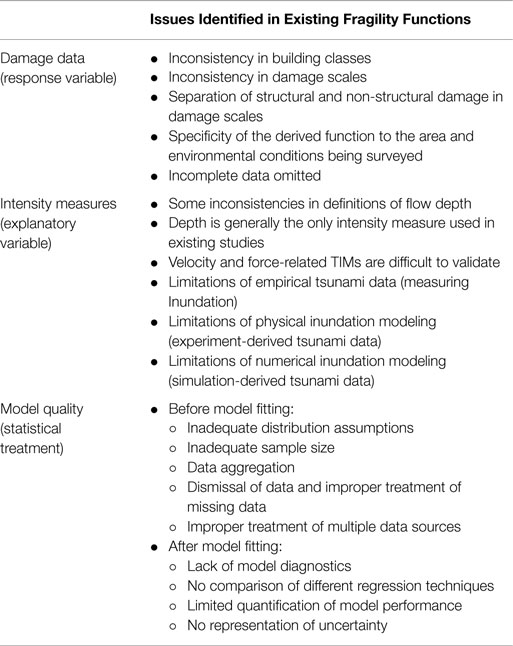
Table 12. Issues with current fragility functions, organized by model component.

Assessment/Improvement of the Quality of Building Damage Data

In order to compare and combine fragility functions, a unification of building classifications for tsunami fragility analysis is needed. Following the example of the seismic building classifications recommended by the GEM (Brzev et al., 2013), it is recommended that tsunami building classifications follow the building attributes that govern performance under tsunami loading as summarized in Table 13.

TABLE 13

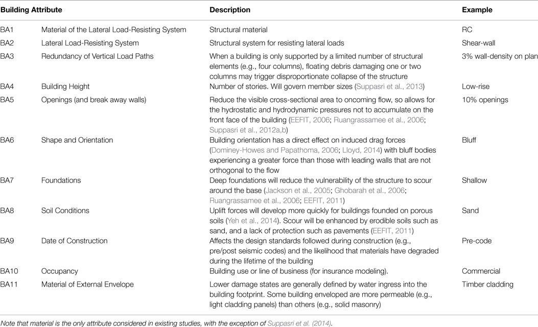
Table 13. Building attributes which govern tsunami performance (BA1-BA10).

Similarly, unification of tsunami damage scales is required and many of the issues highlighted with existing damage scales have been addressed by Fraser et al. (2013) [adapted from EEFIT (2006)] who propose improved damage scales, based on the familiar EMS-98 damage scales, for RC, steel, and timber. This damage scale only goes part way to fulfilling the needs of a damage scale suitable for use in the future development of tsunami fragility functions from both empirical and analytical approaches. Specifically, it includes descriptions of visual damage but does not define a set of engineering demand parameter thresholds that can be used to determine a building’s damage state from an analysis of its tsunami response using software. Hence, research is still required in order to deliver an appropriate damage scale, adhering to the rules set out in Table 3, for use in fragility function derivation.

Typical issues associated with post-tsunami damage data collection have been summarized in Table 6. To obtain more reliable field-survey, data measures must be taken to limit uncertainties due to combining data from surveyors of differing experience, errors in survey forms, or combination of data from different surveys. It is, therefore, necessary to develop universal guidance for tsunami damage data collection. Consistent and adequate training for surveyors is required but may be difficult to achieve for large-scale disasters where a large number of surveyors from different professional backgrounds will be deployed rapidly in the immediate aftermath of the disaster. An example of guidance used for Japanese surveyors following the 2011 Tohoku earthquake and tsunami is presented in EEFIT (2013).

So as not to introduce biases in the data, it is also important to include all buildings in a survey and not segregate data collected to damaged buildings only. Aggregation of data (by location) must also be limited where possible, so as to reduce uncertainty when pairing damage and inundation data. It is recommended that incomplete data are investigated and treated as per Macabuag et al. (2016a).

As empirical fragility functions have been shown to be very sensitive to the location from where their damage data were collected, in order to quantify fragility in the many at-risk locations around the world without available damage data, analytical methods for fragility function derivation based on structural analysis are required.

Assessment/Improvement of the Quality of Tsunami Intensity Data

Although inundation depth is used as the only TIM for the majority of existing tsunami fragility functions, this does not capture all of the relevant tsunami information necessary to predict structural damage. Therefore, for future studies numerical modeling should be conducted in order to obtain TIMs other than depth (validated against values measured or inferred from observations). If the inundation simulation from which they are derived is sufficiently accurate, then force estimates often provide the most efficient TIMs. These and other additional TIMs should be compared and the optimal defined for a given dataset according to the methodology set out in Macabuag et al. (2016a).

Fragility functions incorporating multiple TIMs (e.g., fragility surfaces), should be considered also.

Debris has been shown to significantly affect the fragility of buildings, and further research is needed to fully capture the damage potential that debris presents.

The reliability of the existing fragility functions based on velocity or force is very dependent on the accuracy of the inundation models on which those TIMs are based. Reviewing current best-practice for numerical inundation modeling is outside the scope of this paper, but it is recommended that the quality of inundation models used in existing studies be examined against a number of factors, such as quality/reliability/resolution of the topography/bathymetry data, quality/reliability of the source and propagation models, the software used, the resolution of the calculation grid, and so on.

In order to improve the accuracy of numerical inundation models, better understanding is needed of tsunami near and onshore processes and on the determination of actions on structures. Physical experiments can give an insight into the complex processes involved in flow–structure interactions onshore, however, most large-scale laboratory facilities to-date do not allow for the reproduction of some keys characteristics of tsunami, such as their wavelengths. Some work on tsunami forces has been done using solitary waves or similar, but results involving long (shallow water) waves is limited. This leads to a lack of experimental validation of current fragility and damage relationships. There are several studies to address this gap (Rossetto et al., 2011; Charvet, 2012; Lloyd and Rossetto, 2012; Foster et al., 2017), and this area should be the focus of further research to improve the accuracy of inundation models and the understanding of tsunami-effects on buildings, both crucial for accurate fragility function derivation.

Assessment/Improvement of the Quality of Statistical Modeling

It is recommended that data aggregation be avoided and that missing data be classified and treated prior to regression analysis, as set out in section “Model Quality.”

A case is made to show that existing fragility studies using GLMs are more reliable than those employing linear models with linear least squares parameter estimation. The optimal model configurations for a given dataset can be determined using the tests shown in Table 10. Semi-parametric GAMs may also be used if overfitting is avoided using the cross-validation methods outlined in Macabuag et al. (2016a). If all parametric alternatives fail to provide a satisfactory fit to the data non-parametric regression can be a useful alternative.

For new studies, missing data should be analyzed and treated as set out in Table 11 and it is recommended that existing fragility assessments should be re-examined for potential bias if they have been based on complete-case analysis of data subsets (e.g., construction material).

It is recommended that uncertainty of the mean fragility curves should always be presented and one such technique is to confidence intervals derived by bootstrap methods as outlined in Charvet et al. (2014b). Furthermore, rigorous diagnostics of the final model should be employed in order to assess likely model accuracy.

Multivariate regression can be achieved using GLM regression techniques and any number of intensity measures can be included in the model. However, it is always the aim to develop a “parsimonious model” (the best model for the fewest predictors) as using additional intensity measures requires more data points, and difficulties of obtaining these additional tsunami parameters must be overcome. In addition, the representation of a fragility surface in more than three dimensions (i.e., with more than two TIMs) is challenging and it is necessary to find a representation method giving interpretable and useful results.

Conclusion

This paper collates and summarizes existing empirical tsunami fragility functions for buildings, to outline limitations and significant advances in the field, and to propose key areas for further development. A number of key issues and recommendations for each component of tsunami fragility functions have been presented (damage data, tsunami intensity data, and the statistical model).

The information presented in this paper may be used to assess the quality of current estimations (both based on the quality of the data, and the quality of the models and theories adopted), and to adopt best practice when developing new fragility functions. This paper, therefore, has implications for those using, assessing, or developing tsunami fragility functions.

Author Contributions

IC, early original draft of paper. Author of section on model quality. JM, author of all other sections building on IC’s early draft. Editor of final paper. TR, Reviewer.

Conflict of Interest Statement

The authors declare that the research was conducted in the absence of any commercial or financial relationships that could be construed as a potential conflict of interest.

Acknowledgments

TR’s time is funded by the European Research Council funded URBAN WAVES Starting Grant (reference: 336084). JM’s time is funded by the EPSRC Engineering Doctorate Programme and the Willis Research Network. We would also like to acknowledge the many years of successful collaboration between EPICentre, UCL (UK) and IRIDeS, Tohoku University (Japan) which has made this work possible.

References

Adriano, B., Hayashi, S., Gokon, H., Mas, E., and Koshimura, S. (2016). Understanding the extreme tsunami inundation in Onagawa town by the 2011 Tohoku earthquake, its effects in urban structures and coastal facilities. Coast. Eng. J. 58, 19. doi: 10.1142/S0578563416400131

CrossRef Full Text | Google Scholar

Akaike, H. A. I. (1974). A new look at the statistical model identification. IEEE Trans. Automat. Contr. 19, 716–723. doi:10.1109/TAC.1974.1100705

CrossRef Full Text | Google Scholar

Amakuni, K., and Terazono, N. (2011). “Basic analysis on building damages by tsunami due to the 2011 Great East Japan earthquake disaster using,” in 15 World Conference on Earthquake Engineering. Available at: http://www.iitk.ac.in/nicee/wcee/article/WCEE2012_3628.pdf

Google Scholar

Babyak, M. A. (2004). What you see may not be what you get: a brief, nontechnical introduction to overfitting in regression-type models. Psychosom. Med. 66, 411–421. doi:10.1097/00006842-200405000-00021

CrossRef Full Text | Google Scholar

Bartlett, J. E., Kotrlik, J. W., and Higgins, C. C. (2001). Organizational research: determining appropriate sample size in survey research. Info. Technol. Learn. Perform. J. 19, 43–50.

Google Scholar

Berryman, K. (2005). Review of Tsunami Hazard and Risk in New Zealand. Prepared for (September). Institute of Geological & Nuclear Sciences client report 2005/104, GNS Limited. Available at: http://www.civildefence.govt.nz/assets/Uploads/publications/GNS-CR2005-104-review-of-tsunami-hazard.pdf

Google Scholar

Brzev, S., Charleson, A. W., and Jaiswal, K. (2013). GEM Basic Building Taxonomy Report Produced in the Context of the GEM Ontology and Taxonomy Global Component Project. Available at: http://www.nexus.globalquakemodel.org/gem-building-taxonomy/posts/updated-gem-basic-building-taxonomy-v1.0

Google Scholar

Chandler, R. (2014). “Classical approaches for statistical inference in model calibration with uncertainty,” in Applied Uncertainty Analysis for Flood Risk Management, eds K. Beven, and J. Hall (London: Imperial College Press), 60–67.

Google Scholar

Charvet, I. (2012). Experimental Modelling of Long Elevated and Depressed Waves Using a New Pneumatic Wave Generator. PhD thesis, University College London. Available at: http://discovery.ucl.ac.uk/1343903/1/1343903.pdf

Google Scholar

Charvet, I., Eames, I., and Rossetto, T. (2013). New tsunami runup relationships based on long wave experiments. Ocean Model. 69, 79–92. doi:10.1016/j.ocemod.2013.05.009

CrossRef Full Text | Google Scholar

Charvet, I., Suppasri, A., Kimura, H., Sugawara, D., and Imamura, F. (2015). Fragility estimations for Kesennuma City following the 2011 Great East Japan Tsunami based on maximum flow depths, velocities and debris impact, with evaluation of the ordinal model’s predictive accuracy. Nat. Hazards 79, 2073–2099. doi:10.1007/s11069-015-1947-8

CrossRef Full Text | Google Scholar

Charvet, I., Ioannou, I., Rossetto, T., Suppasri, A., and Imamura, F. (2014a). Empirical fragility assessment of buildings affected by the 2011 Great East Japan tsunami using improved statistical models. Nat. Hazards 73, 951–973. doi:10.1007/s11069-014-1118-3

CrossRef Full Text | Google Scholar

Charvet, I., Suppasri, A., and Imamura, F. (2014b). Empirical fragility analysis of building damage caused by the 2011 Great East Japan tsunami in Ishinomaki city using ordinal regression, and influence of key geographical features. Stoch. Environ. Res. Risk Assess. 28, 1853–1867. doi:10.1007/s00477-014-0850-2

CrossRef Full Text | Google Scholar

Chatterjee, S., and Hadi, A. (2006). Regression Analysis by Example, 4th Edn. Hoboken, NJ, USA: Wiley & Sons.

Google Scholar

Chock, G., Carden, L., Robertson, I., Olsen, M., and Yu, G. (2013). Tohoku tsunami-induced building failure analysis with implications for U.S. tsunami and seismic design codes. Earthq. Spectra 29, S99–S126. doi:10.1193/1.4000113

CrossRef Full Text | Google Scholar

Chock, G. Y. K. (2016). Design for tsunami loads and effects in the ASCE 7-16 standard. J. Struct. Eng. 142, 1–12. doi:10.1061/(ASCE)ST.1943-541X.0001565

CrossRef Full Text | Google Scholar

Cohen, J. (1988). Statistical Power Analysis for the Behavioral Sciences, 2nd Edn. Hillsdale, NJ: Lawrence Erlbaum Associates.

Google Scholar

Crichton, D. (1999). The Risk Triangle. Available at: http://scholar.google.com/scholar?hl=en&btnG=Search&q=intitle:The+risk+triangle#0

Google Scholar

D’Ayala, D., Meslem, A., Vamvatsikos, D., Porter, K., Rossetto, T., Crowley, H., et al. (2013). Guidelines for Analytical Vulnerability Assessment. Available at: http://www.nexus.globalquakemodel.org/gem-vulnerability/posts/guidelines-for-analytical-vulnerability-assessment

Google Scholar

De Risi, R., Goda, K., Mori, N., and Yasuda, T. (2017a). Bayesian tsunami fragility modeling considering input data uncertainty. Stoch. Environ. Res. Risk Assess. 31, 1253–1269. doi:10.1007/s00477-016-1230-x

CrossRef Full Text | Google Scholar

De Risi, R., Goda, K., Yasuda, T., and Mori, N. (2017b). Is flow velocity important in tsunami empirical fragility modeling? Earth Sci. Rev. 166, 64–82. doi:10.1016/j.earscirev.2016.12.015

CrossRef Full Text | Google Scholar

Dias, W. P. S., Yapa, H. D., and Peiris, L. M. N. (2009). Tsunami vulnerability functions from field surveys and Monte Carlo simulation. Civ. Eng. Environ. Syst. 26, 181–194. doi:10.1080/10286600802435918

CrossRef Full Text | Google Scholar

Dominey-Howes, D., and Papathoma, M. (2006). Validating a tsunami vulnerability assessment model (the PTVA model) using field data from the 2004 Indian Ocean tsunami. Nat. Hazards. 40, 113–36. doi:10.1007/s11069-006-0007-9

CrossRef Full Text | Google Scholar

EEFIT. (2006). The Indian Ocean Tsunami of 26 December 2004: Mission Findings in Sri Lanka and Thailand. Field Report by the Earthquake Engineering Field Investigation Team (EEFIT), Institution of Structural Engineers. Available at: http://www.istructe.org/webtest/files/74/74b66946-020a-430d-a684-0f71ff0d2a23.pdf

Google Scholar

EEFIT. (2011). Field Report: Earthquake and Tsunami of 11th March 2011. Field Report by the Earthquake Engineering Field Investigation Team (EEFIT), Institution of Structural Engineers.

Google Scholar

EEFIT. (2013). Field Report (Return Mission): Earthquake and Tsunami of 11th March 2011. Field Report by the Earthquake Engineering Field Investigation Team (EEFIT), Institution of Structural Engineers.

Google Scholar

FEMA. (2012). FEMA P-646: Guidelines for Design of Structures for Vertical Evacuation from Tsunamis, 2nd Edn, Federal Emergency Management Report. Availabale at: https://www.fema.gov/media-library/assets/documents/14708

Google Scholar

Foster, A. S. J., Rossetto, T., and Allsop, W. (2017). An experimentally validated approach for evaluating tsunami inundation forces on rectangular buildings. Coast. Eng. (in press).

Google Scholar

Fraser, S., Raby, A., Pomonis, A., Goda, K., Chian, S. C., Macabuag, J., et al. (2013). Tsunami damage to coastal defences and buildings in the March 11th 2011 M w 9.0 Great East Japan earthquake and tsunami. Bull. Earthq. Eng. 11, 205–239. doi:10.1007/s10518-012-9348-9

CrossRef Full Text | Google Scholar

Ghobarah, A., Saatcioglu, M., and Nistor, I. (2006). The impact of the 26 December 2004 earthquake and tsunami on structures and infrastructure. Eng. Struct. 28, 312–326. doi:10.1016/j.engstruct.2005.09.028

CrossRef Full Text | Google Scholar

Gokon, H., Koshimura, S., and Matsuoka, M. (2009). Developing tsunami fragility curves for structural destruction in American Samoa. J. Jpn. Soc. Civ. Eng. Available at: http://www.enveng.titech.ac.jp/midorikawa/rsdm2010_pdf/04_gokon_paper.pdf

Google Scholar

Gokon, H., Koshimura, S., and Matsuoka, M. (2010). “Developing tsunami fragility curves for structural destruction in American Samoa,” in 8th International Workshop on Remote Sensing for Disaster Response, Tokyo.

Google Scholar

Goseberg, N., Wurpts, A., and Schlurmann, T. (2013). Laboratory-scale generation of tsunami and long waves. Coast. Eng. 79, 57–74. doi:10.1016/j.coastaleng.2013.04.006

CrossRef Full Text | Google Scholar

Green, S. (1991). How many subjects does it take to do a regression analysis? Multivariate Behav. Res. 26, 499–510. doi:10.1207/s15327906mbr2603_7

CrossRef Full Text | Google Scholar

Guadagnoli, E., and Velicer, W. F. (1988). Relation to sample size to the stability of component patterns. Psychol. Bull. 103, 265–275. doi:10.1037/0033-2909.103.2.265

CrossRef Full Text | Google Scholar

Harrell, F. E. Jr., Lee, K. L., Matchar, D. B., and Reichert, T. A. (1985). Regression models for prognostic prediction: advantages, problems, and suggested solutions. Cancer Treat. Rep. 69, 1071–1077.

PubMed Abstract | Google Scholar

Hastie, T., and Tibshirani, R. (1990). Generalized Additive Models, Chapman & Hall/CRC Monographs on Statistics & Applied Probability. Available at: http://www.amazon.co.uk/Generalized-Additive-Monographs- Statistics-Probability/dp/0412343908

Google Scholar

Hayashi, S., Narita, Y., and Koshimura, S. (2013). Developing tsunami fragility curves from the surveyed data and numerical modeling of the 2011 Tohoku earthquake tsunami (in Japanese). J. Jpn. Soc. Civ. Eng. Coast. Eng. 69, 1–5. doi:10.2208/kaigan.69.I_386

CrossRef Full Text | Google Scholar

Hill, M., and Rossetto, T. (2008). Comparison of building damage scales and damage descriptions for use in earthquake loss modelling in Europe. Bull. Earthq. Eng. 6, 335–365. doi:10.1007/s10518-007-9057-y

CrossRef Full Text | Google Scholar

Inoue, S., Wijeyewickrema, A. C., and Matsumoto, H. (2007). “Field survey of tsunami effects in Sri Lanka due to the Sumatra-Andaman earthquake of December 26, 2004,” in Tsunami and Its Hazards in the Indian and Pacific Ocean (Basel: Springer), 395–411.

Google Scholar

Ioannou, I., Rossetto, T., and Grant, D. N. (2012). “Use of regression analysis for the construction of empirical fragility curves,” in 15 World Conference on Earthquake Engineering. Available at: http://www.iitk.ac.in/nicee/wcee/article/WCEE2012_2143.pdf

Google Scholar

Jackson, L. E., Vaughn Barrie, J., Forbes, D. L., Shaw, J., Manson, G. K., and Schmidt, M. (2005). Effects of the 26 December 2004 Indian Ocean Tsunami in the Republic of Seychelles. Report of the Canada-UNESCO Indian Ocean Tsunami Expedition 19 January–5 February 2005. Available at: http://www.unisdr.org/files/2193_VL323132.pdf

Google Scholar

Japan Cabinet Office. (2013). Residential Disaster Damage Accreditation Criteria Operational Guideline. Available at: http://www.bousai.go.jp/taisaku/unyou.html

Google Scholar

Kircher, C. A., and Bouabid, J. (2014). “New building damage and loss functions for Tsunami,” in 10th International Conference on Urban Earthquake Engineering (Tokyo).

Google Scholar

Koshimura, S., and Gokon, H. (2012). Structural vulnerability and tsunami fragility curves from the 2011 Tohoku earthquake tsunami disaster. J. Jpn. Soc. Civ. Eng. Ser. B2 (Coast. Eng.) 68, I_336–I_340. doi:10.2208/kaigan.68.I_336

CrossRef Full Text | Google Scholar

Koshimura, S., and Kayaba, S. (2010). Tsunami fragility inferred from the 1993 Hokkaido Nansei-oki earthquake tsunami disaster. J. Jpn. Assoc. Earthq. Eng. 10, 87–101. doi:10.5610/jaee.10.3_87

CrossRef Full Text | Google Scholar

Koshimura, S., Namegaya, Y., and Yanagisawa, H. (2009a). Tsunami fragility – a new measure to identify tsunami damage. J. Disaster Res. 4, 479–488. doi:10.20965/jdr.2009.p0479

CrossRef Full Text | Google Scholar

Koshimura, S., Oie, T., Yanagisawa, H., and Imamura, F. (2009b). Developing fragility functions for tsunami damage estimation using numerical model and post-tsunami data from Banda Aceh, Indonesia. Coast. Eng. J. 51, 243–273. doi:10.1142/S0578563409002004

CrossRef Full Text | Google Scholar

Kreibich, H., Piroth, K., Seifert, I., Maiwald, H., Kunert, U., Schwarz, J., et al. (2009). Is flow velocity a significant parameter in flood damage modelling? Nat. Hazards Earth Syst. Sci. 9, 1679–1692. doi:10.5194/nhess-9-1679-2009

CrossRef Full Text | Google Scholar

Kriebel, D. L., Lynett, P. J., Cox, D. T., Petroff, C. M., Robertson, I. N., and Chock, G. Y. K. (2017). Energy method for approximating overland tsunami flows. J. Waterw. Port Coast. Ocean Eng. 143. Available at: http://ascelibrary.org/doi/abs/10.1061/%28ASCE%29WW.1943-5460.0000393

Google Scholar

Leelawat, N., Suppasri, A., Charvet, I., and Imamura, F. (2014). Building damage from the 2011 Great East Japan tsunami: quantitative assessment of influential factors. Nat. Hazards 73, 449–471. doi:10.1007/s11069-014-1081-z

CrossRef Full Text | Google Scholar

Lloyd, T. O. (2014). An Experimental Investigation of Tsunami Forces on Coastal Structures. London: University College London.

Google Scholar

Lloyd, T. O., and Rossetto, T. (2012). “A comparison between existing tsunami load guidance and large-scale experiments with long-waves,” in 15 World Conference on Earthquake Engineering (Lisbon).

Google Scholar

Macabuag, J., and Rossetto, T. (2014). “Towards the development of a method for generating analytical tsunami fragility functions,” in 2nd European Conference on Earthquake Engineering and Seismology.

Google Scholar

Macabuag, J., Rossetto, T., and Ioannou, I. (2016a). “Investigation of the effect of debris-induced damage for constructing tsunami fragility curves for buildings,” in 1st International Conference on Natural Hazards & Infrastructure (Chania, Greece).

Google Scholar

Macabuag, J., Rossetto, T., Ioannou, I., Suppasri, A., Sugawara, D., Adriano, B., et al. (2016b). A proposed methodology for deriving tsunami fragility functions for buildings using optimum intensity measures. Nat. Hazards 84, 1257–1285. doi:10.1007/s11069-016-2485-8

CrossRef Full Text | Google Scholar

Maruyama, Y., Kitamura, K., and Yamazaki, F. (2013). “Tsunami damage assessment of buildings in Chiba Prefecture, Japan using fragility function developed after the 2011 Tohoku-Oki earthquake,” in Safety, Reliability, Risk and Life-Cycle Performance of Structures & Infrastructures (Taylor & Francis). Available at: http://ares.tu.chiba-u.jp/~papers/paper/2013/2013ICOSSAR_Maruyama.pdf

Google Scholar

Mas, E., Koshimura, S., Suppasri, A., Matsuoka, M., Matsuyama, M., Yoshii, T., et al. (2012). Developing Tsunami fragility curves using remote sensing and survey data of the 2010 Chilean Tsunami in Dichato. Nat. Hazards Earth Syst. Sci. 12, 2689–2697. doi:10.5194/nhess-12-2689-2012

CrossRef Full Text | Google Scholar

Masuda, M., Williams, C., Shahkarami, A., and Bryngelson, F. R. J. (2012). “Tsunami vulnerability function development based on the 2011 Tohoku earthquake in Japan,” in 15 World Conference on Earthquake Engineering (Lisbon).

Google Scholar

McCullagh, P., and Nelder, J. A. (1983). Generalized Linear Models, 2nd Edn. Available at: https://books.google.co.uk/books/about/Generalized_Linear_Models_Second_Edition.html?id=h9kFH2_FfBkC&pgis=1

Google Scholar

McCullagh, P., and Nelder, J. A. (1989). Generalized Linear Models, 2nd Edn, Chapman & Hall/CRC.

Google Scholar

Miller, L. E., and Kunce, J. T. (1973). Prediction and statistical overkill revisited. Meas. Eval. Guid. 6, 157–163.

Google Scholar

MLIT. (2011). Concerning Setting the Safe Structure Method for Tsunamis Which Are Presumed When Tsunami Inundation Occurs – Public Notice 1318. Ministry of Land, Infrastructure, Transportation and Tourism (in Japanese).

Google Scholar

Muhari, A., Charvet, I., Tsuyoshi, F., Suppasri, A., and Imamura, F. (2015). Assessment of tsunami hazards in ports and their impact on marine vessels derived from tsunami models and the observed damage data. Nat. Hazards 78, 1309–1328. doi:10.1007/s11069-015-1772-0

CrossRef Full Text | Google Scholar

Muhari, A., Imamura, F., Koshimura, S., and Post, J. (2011). Examination of three practical run-up models for assessing tsunami impact on highly populated areas. Nat. Hazards Earth Syst. Sci. 11, 3107–3123. doi:10.5194/nhess-11-3107-2011

CrossRef Full Text | Google Scholar

Murao, O., and Nakazato, H. (2010). “Vulnerability functions for buildings based on damage survey data in Sri Lanka after the 2004 Indian Ocean tsunami,” in International Conference on Sustainable Built Environment (ICSBE-2010) Kandy, 371–378.

Google Scholar

Myung, I. J. (2003). Tutorial on maximum likelihood estimation. J. Math. Psychol. 47, 90–100. doi:10.1016/S0022-2496(02)00028-7

CrossRef Full Text | Google Scholar

Narita, Y., and Koshimura, S. (2015). Classification of tsunami fragility curves based on regional characteristics of tsunami damage. J. Jpn. Soc. Civ. Eng. Coast. Eng. 71, 331–336. doi:10.2208/kaigan.71.I_331

CrossRef Full Text | Google Scholar

Nihei, Y., Maekawa, T., Ohshima, R., and Yanagisawa, M. (2012). Evaluation of fragility functions for tsunami damage in coastal district in Natori City, Miyagi Prefecture and mitigation effects of coastal dune. J. Jpn. Soc. Civ. Eng. 68, I_276–I_280. doi:10.2208/kaigan.68.I_276

CrossRef Full Text | Google Scholar

Noh, H. Y., Lallemant, D., and Kiremidjian, A. S. (2014). Development of empirical and analytical fragility functions using kernel smoothing methods. Earthq. Eng. Struct. Dyn. Available at: http://faculty.ce.cmu.edu/noh/files/2016/02/Noh_EESD2_published_eqe2505.pdf

Google Scholar

Nunnally, J. C., and Bernstein, I. H. (1994). Psychometric Theory, 3rd Edn. USA: McGraw-Hill, Inc.

Google Scholar

Park, H., Wiebe, D., and Cox, D. T. (2014). Tsunami inundation modeling: sensitivity of velocity and momentum flux to bottom friction with application to building damage at Seaside, Oregon. Coast. Eng. 1–12. Available at: https://icce-ojs-tamu.tdl.org/icce/index.php/icce/article/view/7557/pdf_985

Google Scholar

Park, S., van de Lindt, J. W., Cox, D., and Gupta, R. (2013). Concept of community fragilities for tsunami coastal inundation studies. Nat. Hazards Rev. 14, 220–228. doi:10.1061/(ASCE)NH.1527-6996.0000092

CrossRef Full Text | Google Scholar

Pomonis, A., and Peiris, N. (2005). “December 26, 2004 Indian Ocean tsunami: vulnerability functions for loss estimation in,” in International Conference on Geotechnical Engineering for Disaster Mitigation & Rehabilitation (Singapore), 411–416.

Google Scholar

Pringle, W., and Yoneyama, N. (2013). The application of a hybrid 2D/3D numerical tsunami inundation-propagation flow model to the 2011 off the Pacific Coast of Tohoku earthquake tsunami. J. Jpn. Soc. Civ. Eng. Coast. Eng. 63, 3–7. doi:10.2208/kaigan.69.I_306

CrossRef Full Text | Google Scholar

Qi, Z. X., Eames, I., and Johnson, E. R. (2014). Force acting on a square cylinder fixed in a free-surface channel flow. J. Fluid Mech. 756, 716–727. doi:10.1017/jfm.2014.455

CrossRef Full Text | Google Scholar

Reese, S., Bradley, B. A., Bind, J., Smart, G., Power, W., and Sturman, J. (2011). Empirical building fragilities from observed damage in the 2009 South Pacific tsunami. Earth Sci. Rev. 107, 156–173. doi:10.1016/j.earscirev.2011.01.009

CrossRef Full Text | Google Scholar

Reese, S., Cousins, W. J., Power, W. L., Palmer, N. G., Tejakusuma, I. G., and Nugrahadi, S. (2007). Tsunami vulnerability of buildings and people in South Java – field observations after the July 2006 Java tsunami. Nat. Hazards Earth Syst. Sci. 7, 573–589. doi:10.5194/nhess-7-573-2007

CrossRef Full Text | Google Scholar

Robertson, I. N., and Riggs, H. R. (2011). “OMAE2011-49487 tsunami bore forces on walls,” in Proceedings of the ASTM 2011 30th Internal Conference on Ocean, Offshore and Arctic Engineering (Rotterdam).

Google Scholar

Rossetto, T., Allsop, W., Charvet, I., and Robinson, D. I. (2011). Physical modelling of tsunami using a new pneumatic wave generator. Coast. Eng. 58, 517–527. doi:10.1016/j.coastaleng.2011.01.012

CrossRef Full Text | Google Scholar

Rossetto, T., Ioannou, I., Grant, D. N., and Maqsood, T. (2014). Guidelines for Empirical Vulnerability Assessment: Report Produced in the Context of the Vulnerability Global Component Project. Pavia: GEM Technical Report 2014-08, GEM Foundation.

Google Scholar

Rossetto, T., Ioannou, I., and Grant, D. (2012). Guidelines for Empirical Vulnerability Assessment – Phase I: Single Surveys. Pavia: GEM Technical Report 2012-X, GEM Foundation.

Google Scholar

Ruangrassamee, A., Yanagisawa, H., Foytong, P., Lukkunaprasit, P., Koshimura, S., and Imamura, F. (2006). Investigation of tsunami-induced damage and fragility of buildings in Thailand after the December 2004 Indian Ocean tsunami. Earthq. Spectra 22, 377–401. doi:10.1193/1.2208088

CrossRef Full Text | Google Scholar

Rubin, D. (1987). Multiple Imputation for Nonresponse in Surveys. John Wiley & Sons.

Google Scholar

Satake, K., Fujii, Y., Harada, T., and Namegaya, Y. (2013). Time and space distribution of coseismic slip of the 2011 Tohoku earthquake as inferred from tsunami waveform data. Bull. Seismol. Soc. Am. 103, 1473–1492. doi:10.1785/0120120122

CrossRef Full Text | Google Scholar

Schuenemeyer, J., and Drew, L. (2011). Statistics for Earth and Environmental Scientists. John Wiley & Sons.

Google Scholar

Scott, M. H., and Mason, H. B. (2017). Constant-ductility response spectra for sequential earthquake and tsunami loading. Earthq. Eng. Struct. Dyn. 46, 1549–1554.

Google Scholar

Synolakis, C. E., Bernard, E. N., Titov, V. V., Kânoglu, U., and González, F. I. (2008). Validation and verification of tsunami numerical models. Pure Appl. Geophys. 165, 2197–2228. doi:10.1007/s00024-004-0427-y

CrossRef Full Text | Google Scholar

Suppasri, A., Charvet, I., Imai, K., and Imamura, F. (2014). Fragility curves based on data from the 2011 Great East Japan tsunami in Ishinomaki city with discussion of parameters influencing building damage. Earthq. Spectra 31, 841–868. doi:10.1193/053013EQS138M

CrossRef Full Text | Google Scholar

Suppasri, A., Koshimura, S., Imai, K., Mas, E., Gokon, H., Muhari, A., et al. (2012a). Damage characteristic and field survey of the 2011 Great East Japan tsunami in Miyagi Prefecture. Coast. Eng. J. 54, 30. doi:10.1142/S0578563412500052

CrossRef Full Text | Google Scholar

Suppasri, A., Koshimura, S., and Imamura, F. (2009). “Tsunami fragility curves and structural performance of building along the Thailand coast,” in 8th International Workshop on Remote Sensing for Disaster Management (Tokyo), 3–8.

Google Scholar

Suppasri, A., Koshimura, S., and Imamura, F. (2011). Developing tsunami fragility curves based on the satellite remote sensing and the numerical modeling of the 2004 Indian Ocean tsunami in Thailand. Nat. Hazards Earth Syst. Sci. 11, 173–189. doi:10.5194/nhess-11-173-2011

CrossRef Full Text | Google Scholar

Suppasri, A., Latcharote, P., Bricker, J. D., Leelawat, N., Hayashi, A., Yamashita, K., et al. (2016). Improvement of tsunami countermeasures based on lessons from the 2011 Great East Japan earthquake and tsunami – situation after five years. Coast. Eng. J. 58, 1640011. doi:10.1142/S0578563416400118

CrossRef Full Text | Google Scholar

Suppasri, A., Mas, E., Charvet, I., Gunasekera, R., Imai, K., Fukutani, Y., et al. (2013). Building damage characteristics based on surveyed data and fragility curves of the 2011 Great East Japan tsunami. Nat. Hazards 66, 319–341. doi:10.1007/s11069-012-0487-8

CrossRef Full Text | Google Scholar

Suppasri, A., Mas, E., Koshimura, S., et al. (2012b). Developing tsunami fragility curves from the surveyed data of the 2011 Great East Japan tsunami in Sendai and Ishinomaki plains. Coast. Eng. J. 54, 16. doi:10.1142/S0578563412500088

CrossRef Full Text | Google Scholar

Tanaka, N., and Kondo, K. (2015). Numerical analysis considering the effect of trapping the floatage by coastal forests and fragility curve of houses. J. Jpn. Soc. Civil Eng. Ser. B1 (Hydraul Eng). 71, I_727–I_732. doi:10.2208/jscejhe.71.I_727

CrossRef Full Text | Google Scholar

Tanaka, N., Onai, A., and Kondo, K. (2015). Fragility curve of different damage of wooden building due to tsunami based on tsunami fluid force and its moment (in Japanese). J. Jpn. Soc. Civ. Eng. Coast. Eng. 71, 1–11. doi:10.2208/kaigan.71.1

CrossRef Full Text | Google Scholar

Tanaka, N., Sasaki, Y., Mowjood, M. I. M., Jinadasa, K. B. S. N., and Homchuen, S. (2007). Coastal vegetation structures and their functions in Tsunami protection: experience of the recent Indian Ocean Tsunami. Landscape Ecol. Eng. 33–45.

Google Scholar

Tarbotton, C., Dall’Osso, F., Dominey-Howes, D., and Goff, J. (2015). The use of empirical vulnerability functions to assess the response of buildings to tsunami impact: comparative review and summary of best practice. Earth Sci. Rev. 142, 120–134. doi:10.1016/j.earscirev.2015.01.002

CrossRef Full Text | Google Scholar

Tinti, S., Tonini, R., Bressan, L., Armigliato, A., Gardi, A., Guillande, R., et al. (2011). Handbook of Tsunami Hazard and Damage Scenarios (EUR 24691 EN). Available at: http://publications.jrc.ec.europa.eu/repository/bitstream/111111111/16149/1/lbna24691enc.pdf

Google Scholar

Tokyo University and BRI. (2011). Interim Report of the Building Standards Improvement Promotion Project No. 40, A Study of Improvement of Building Standards etc in the Tsunami Critical Areas.

Google Scholar

Valencia, N., Gardi, A., Gauraz, A., Leone, F., and Guillande, R. (2011). New tsunami damage functions developed in the framework of SCHEMA project: application to European-Mediterranean coasts. Nat. Hazards Earth Syst. Sci. 11, 2835–2846. doi:10.5194/nhess-11-2835-2011

CrossRef Full Text | Google Scholar

VanVoorhis, C. R. W., and Morgan, B. (2007). Understanding power and rules of thumb for determining sample sizes. Tutorials Quant. Methods Psychol. 3, 43–50. doi:10.20982/tqmp.03.2.p043

CrossRef Full Text | Google Scholar

Ware, J. H., Harrington, D., Hunter, D. J., and D’Agostino, R. B. (2012). Missing data. N. Engl. J. Med. 367, 1353–1354. doi:10.1056/NEJMsm1210043

CrossRef Full Text | Google Scholar

Wood, S. (2006). Generalized Additive Models: An Introduction with R. London: CRC Press.

Google Scholar

Yamazaki, Y., and Cheung, K. (2011). Shelf resonance and impact of near-field tsunami generated by the 2010 Chile earthquake. Geophys. Res. Lett. 38. doi:10.1029/2011GL047508

CrossRef Full Text | Google Scholar

Yanagisawa, H., and Yanagisawa, H. (2012). Fragility function of house damage by the 2011 off the Pacific Coast of Tohoku earthquake tsunami. J. Jpn. Soc. Civ. Eng. Ser. B2 Coast. Eng. 68, I_1401–I_1405. doi:10.2208/kaigan.68.I_1401

CrossRef Full Text | Google Scholar

Yeh, H., Barbosa, A. R., Ko, H., and Cawley, J. G. (2014). Tsunami loadings on structures: review and analysis. Coast. Eng. Proc. 34. Available at: https://icce-ojs-tamu.tdl.org/icce/index.php/icce/article/view/7955

Google Scholar